Abstract
Land use significantly influences the planet’s land surface and associated biogeochemical processes. With fierce conflict between various land uses, it is important to project the land system process to support decision-making. Lack of insight into scale differences of land use change (LUC) increased uncertainties in previous studies. To quantify the differences in LUCs within an elevation gradient, in this study, a novel model, the stratified land use change simulation model (SLUCS), was developed by using an elevation-based stratification strategy. This model consists of four modules. First, an elevation-based stratification module to develop a quantitative method for generating stratifications using elevation and land-use characteristics. Second, a non-spatial land-use demand module to forecast the overall land use area and make zoning constraints to simulate LUCs. Third, a stratified suitability estimation module that uses the stratified logistic regression method to reveal the regional relationship of the driving factors with LUCs at different stratifications. Finally, a spatial allocation of the land-use module, which projects a spatially explicit LUC. The SLUCS model was applied and tested in the Guizhou and Guangxi Karst Mountainous Region. Results validated the effectiveness of the model, and further demonstrated an improved spatial consistency with the reference, a higher accuracy assessment, and a better simulation performance in conversion areas than the traditional method. Three scenarios from 2015 to 2030 with different land-use priorities were designed and projected. Each scenario presented the same LUC trends, but with different magnitudes, including the rapid expansion of built-up land, the restoration of forest and water, and the loss of farmland and grassland. Priority of the socioeconomic development and ecological protection of the scenarios forecasted a sharper increase in the built-up land and in forests than the historical extrapolation scenario. The SLUCS model visually projected the LUC trajectory and competition between land uses, which suggests specific tradeoffs among management strategies to support sustainable land uses.
1. Introduction
Land-use activities, activities converting natural landscapes for human use or changing management practices on human-dominated lands, have transformed the planet’s land surface [1,2]. At the global scale, land is becoming a scarce resource, which leads to the fierce competition and conflict between various groups of people [3]. The world has experienced a large-scale cropland expansion and intensification to meet food demands for the growing population in the last centuries [4]. Also, the conversion of Earth’s land surface to urban uses drives the loss of farmland, affects local climate, fragments habitats, and threatens biodiversity [5]. Meanwhile, afforestation/reforestation projects have been implemented to mitigate climate change and sustain land systems [6]. For example, 16 sustainability programs have improved the sustainability of land systems in China [7]. Land use, as a force of global importance, significantly influences the atmosphere, pedosphere, hydrosphere, and biosphere of the earth [8], and its change results in climatic, biological, and socio-political forces [9,10]. With different demands for economic growth, population growth, and ecological restoration and protection, modeling and projecting land-use change processes is necessary to support the design and implementation of land-use planning and policy.
Previous studies have elaborately reviewed the multiple available models of simulating land-use change, which were developed and applied to provide a platform for both emulating mechanisms of land-change processes by the computer encodes and making projections of future land-cover and land-use patterns [10,11,12,13]. Models have ranged from those using pattern-based methods to structural or process-based methods [14,15]. Brown, Verburg, Pontius and Lange [14] identified five key types of modeling approaches according to the model input, output, and land use conversion rule design. The models quantify the complex relationships between physical factors, human activities, and land-use dynamics, and simulate the land system process under different strategies [14,15]. Under the combined influences of these factors with different spatial patterns, the land use change would constitute an obviously spatial-explicit discrimination. In this way, the land use simulation models, setting the uniform rules of land use change in the model design, tend to lose the detailed spatial characteristics of land use conversion in the previous studies. Therefore, it is necessary to incorporate relevant regional difference information for simulating the land use dynamics.
To better project the future land-use change, precisely quantifying the complicated impact of the driving factors is necessary. However, land-use changes differ with driving factors by region [12,16]. Global scale assessments may therefore conflict with the findings of micro- or meso-scale data sets [9]. In this case, the demands for land resources would be different and conflicted at different stakeholders and scales [17]. To take the scale dependency into account, a separate simulation method was used for different world regions in the global land-use projection [16,18]. Within regional research of land-use change, few studies have focused on this issue, which leads to scale biases and simulation uncertainties. In particular, mountain ecosystems, characterized by their topographic and climatic variety, presented shifts in land-use change across their elevation gradient [19]. Meteorological variables, soil properties, and vegetative functions change with the elevation in the mountainous area [20,21], and further the human activities and demands on the land use are influenced the elevation [19,22]. Previous study only used the elevation as one of driving forces, but limited studies measure the difference of land use dynamics within different elevation gradients. To quantify the regional differences of land-use changes [23], it call for an insight into spatially varying process of land-use change in the model design. Using the elevation gradients as zoning constraints, demands for the land and land use functional orientations are spatial-differentially depicted, and further regional relationships between driving factors and land use are quantified by the stratified strategy in this study. This can help better understand the land system dynamics and improve the simulation accuracy.
Stratifications provide a useful approach to simplifying heterogeneity, which divides environmental gradients into convenient units and then to uses these as sub-regions with relatively consistent characteristics [24]. Traditional stratification is subjectively based on expert knowledge [25] or a statistical clustering of environmental variables [26,27]. Knowledge of stratification approaches for the projection of land-use change is limited and unclear. Object-based segmentation methods provide an innovative way for image analysis to develop observation units with a set of similar pixels [28,29], which would be potentially useful in a stratified strategy for simulating land system dynamics. Thus, the objective of this study was to (1) develop an enhanced land-use change simulation model with an elevation-based stratification strategy; and (2) apply the new model to simulate land-use change and investigate the model performance. The model contributes to the existing body of literature on getting a better approximation for spatial land use change pattern and an improvement of model simulation performance. This would enhance the understanding of land use dynamics process and provide a more reliable output to support for the decision making.
2. Materials and Methods
2.1. Study Area
The Guizhou and Guangxi Karst Mountainous Region, a typical karst region in southwestern China, was selected as the case-study area (Figure 1). Fengcong and fenglin, the two major types of karst terrain [30], are widely disturbed in the study area. Fenglin is the most extreme form of karst landscape, and much of it may evolve from fengcong. Fengcong, translating as peak cluster, is a karst with roughly conical hills separated by deep closed depressions forming a continuous terrain of steep slopes and significant relief; and fenglin, translating as peak forest, is a karst with isolated hills rising from a plain forming of limestone bedrock overlain by a veneer of alluvium [30]. The elevation ranges from 0 to 2848 m with a gradually decreasing gradient from northwest to southeast [31]. It was found that the vertical terrain features affect the land-use change in the study area [31]. Thus, they can be used for testing the hypothesis for the elevation-based stratified simulation strategy and for validating the model performance.
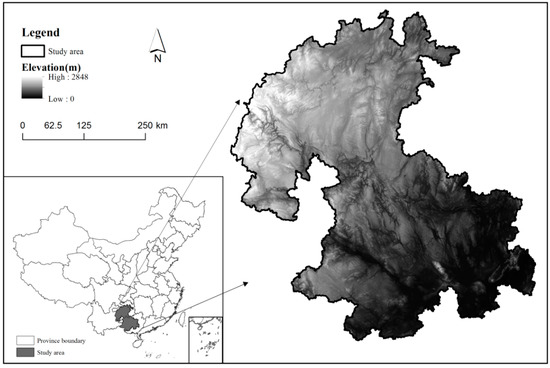
Figure 1.
Location of Guizhou and Guangxi Karst Mountainous Region, China.
The study area is roughly located between 22°8′54′′N–28°12′27′′N and 104°18′27′′E–110°20′40′′E and encompasses the majority of Guizhou and Guangxi provinces in China. The area covers 211,400 km2 and lies within the subtropical monsoon humid climate zone with a mean annual temperature of 19 °C and a mean annual precipitation of 1350 mm. According to the Genetic Soil Classification of China [32], terra fusca, yellow soil, and red soil are the three principal soil types in the study area.
2.2. Land-Use System and Driving Factors
China’s Land-Use/cover Datasets, provided by the Data Center for Resources and Environmental Sciences at the Chinese Academy of Sciences, were used in this study. The average interpretation accuracy of out-door surveys and random sample checks were 92.9% and 97.6%, respectively [33], which consisted of 6 first levels and 25 levels of land-use categories in total. We reclassified the land-use system in this study as seven categories: Paddy field, dry land, forest, grassland, water, built-up land, and bare land.
According to driving factors used by Huang and Cai [34] and Liu, et al. [35], seven aspects, including seventeen variables, were selected for analyzing their relationship to land-use change, calibrating and validating the model in Table 1. The climatic factors include temperature and precipitation. Soil types, texture, and organic matter were chosen to characterize the effect of soil property on land use. Vegetation types and the Normalized Difference Vegetation Index (NDVI) were used to represent the vegetative factors. The MODIS NDVI (MOD13Q3) provided every 16 days at the spatial resolution of 250 m was selected. The datasets were preprocessed with the Atmosphere Bidirectional Reflectance Distribution Function (BRDF) Correction [36] and geometric correction was resampled using a nearest neighbor operator from their native sinusoidal projection to the Albers equal-area conic projection. The maximum value composite method was used to produce the monthly NDVI values and the annual value was calculated by the average values of twelve months. Then the average annual NDVI between 2001 and 2005 was calculated and used. Topographic factors included the elevation and slope. The aspect was calculated using the elevation data from Shuttle Radar Topography Mission (SRTM) Digital Elevation Model dataset and ArcGIS 10.1 (ESRI Inc., Redlands, CA, USA). The karst rocky desertification class characterize the influence of land degradation on the land-use change. Population density and gross domestic product (GDP) were selected as the two socio-economic factors. Location factors, including the distance to roads, distance to settlements, and distance to rivers, were selected. Distances to roads and settlements were the proxies for the distribution of human activities [37], assuming that a shorter distance to roads and settlements indicated an increased human influence. The distance to rivers reflected the accessibility of water resources and fishery products [38,39]. To forecast the land use in 2030, temporal scale of several driving data were updated from the same data sources, including the temperature and precipitation from 1995–2015, NDVI from 2011 to 2015, population density and GDP in 2015, and road in 2015. Other factors were used as the same data in Table 1. All the data were resampled in the WGS84 projection constrained by the same boundary of the study area in GIS 10.1 with a pixel size of 1000 m × 1000 m.

Table 1.
Data sources and description of driving forces.
2.3. Overall Model Structure
The novelty of this study to establish an enhanced land-use change simulation model by the elevation-based stratification strategy (SLUCS). SLUCS consists of four modules: (a) Elevation-based stratification; (b) non-spatial land-use demand; (c) stratified suitability estimation; and (d) spatial allocation of land use (Figure 2). This model can produce the elevation-based stratifications coupling with the land use characteristics. Then it would project land system dynamics at these stratifications, which can make zoning constraints to simulate land sue changes with different land utilization orientations and use the stratified logistic regression method to reveal the regional relationship of the driving factors with land uses at different stratifications. The model is hypothesized to get a better approximation for the land use dynamics process and an improvement of model performance. To achieve this, the elevation-based stratification module divided the study area into several spatially-continuous stratifications to separately simulate the land-use change within a stratified structure. A non-spatial land-use demand module calculates overall areas of all land-use types in each sub-region for input into the model. The stratified suitability estimation module quantifies the relationship between land use and driving factors at stratified sub-regions while still being globally relevant. Finally, the spatial allocation of the land-use module projected the land use at each location for the spatially explicit output.
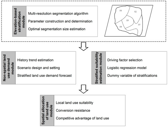
Figure 2.
Overall structure of the elevation-based stratification strategy (SLUCS) model.
The elevation-based stratification module utilized the object-based segmentation tool to determine the division of stratifications. Using the multi-resolution segmentation algorithm from the eCognition 8.0 software [42], the object-based segmentation was performed by using the elevation data. Based on the land-use characteristics of the stratifications, three parameters were proposed to evaluate the intra-segment homogeneity and inter-segment heterogeneity of the stratifications and determine the optimal segmentation.
The non-spatial land-use demand module calculated the statistical demand of different land-use types without the spatial dimension. The module estimated the aggregated quantity of land-use demands using the statistical method and scenario setting. To project the future land-use change, the Markov chain model [43] was used to forecast the historic trend of land-use change and designed varying scenarios according to different priorities and demands for land use. Based on the stratified forecast of historical land-use trends, the non-spatial land-use demands in the entire study area was divided at different stratifications under varying scenario settings.
The stratified suitability estimation module analyzed the relationship between the land use and driving factors based on the divided stratifications from the elevation-based stratification module. Given the uncertainty of land-use dynamics, it is feasible to express the conversion potential of a location with probability rules rather than deterministic rules [44]. Thus, this study used a logistic regression model with dummy variables in order to label various stratifications [45] and to quantify the stratified relationship between land use and driving factors.
The spatial allocation of the land-use module projected each location to the highest conversion potential of the land-use types, which then used the iterative techniques to make the spatially aggregated land-use quantity consistent with the result of the non-spatial module. Using the strategy in the widely used the Conversion of Land Use and its Effects at Small regional extents model (CLUE-S) [46], the module determined the spatial allocation based on the conversion potential possibility. The spatial allocation was summed by three parts: The local land-use suitability from stratified the suitability estimation module, the conversion resistance, and the competitive advantage of the land use.
2.3.1. Elevation-Based Stratification Module
The elevation-based stratification module was executed according to the object-based segmentation tool in the eCognition 8.0 software, which has successfully performed the segmentation and divided images as different objects in previous studies [47,48]. The objects were labeled as stratifications with the same meaning in this study. The multi-resolution segmentation algorithm, including the three parameters of shape, compactness, and scale, was used in this study. The shape defines the homogeneity of the stratification values influencing the size, length, and edge complexity [49], while compactness is defined as the ratio of the border length and the square root of the number of pixel compactness [50]. According to previous studies [47,48], the selected shape and compactness parameters were set to a default of 0.1 and 0.5 in the eCognition software. The scale parameter influences how large the stratifications can grow, thus influencing the number of pixels that can be grouped into a stratification [49]. The elevation data were used for the execution of eCognition with different scale parameters.
To ensure the stratification was not over-segmented or under-segmented, rules were needed to validate an optimal segmentation scale. The optimal image segmentation scale was defined as the scale that maximized intra-segment homogeneity and inter-segment heterogeneity [51]. Especially, land-use characteristics in each stratification would be similar, but significantly different from each other in the model. Therefore, too many or too few stratifications would not adequately project the land-use change and may also lead to scale biases. We assigned a step size of 500 and a range of 0–10,000 for the particular scale parameter changes to produce the multi-scale segmented stratifications. A larger scale parameter produced a larger area of stratification. Using the stratifications with different parameter settings and the land-use map, each land-use proportion within the stratification unit can be calculated. Afterwards, three indicators to find the optimal segmentation scale were proposed.
On one hand, the intra-segment homogeneity should ensure that features of interest were not grouped into stratifications represented by other features. To prevent this, the homogeneity of each stratification was taken into consideration to identify the optimal segmentation level. The homogeneity was defined as the sum of the area-weighted standard deviation of each stratification (ASDintra) for each segmentation level using the follow equation:
where Ni is the number of stratifications; is the area of each stratification; and is the standard deviation of all land-use-area proportions in each stratification. A higher ASDintra indicated a smaller intra-segment homogeneity within all segmented stratifications.
On the other hand, the inter-segment heterogeneity would ensure features were significantly different from their neighbors. The optimal segmentation size can be estimated by making advances of local variance [41]. The local variance was defined as the mean standard deviation of the stratifications (LVinter) through segmentation to explore the heterogeneity of all stratifications for each segmentation scale level:
where Nj is the number of the land-use type (Nj = 7 in this study); j denotes the land-use type (such as paddy field, dry land, forest, grassland, water, built-up area, and bare land); mij is the j land-use proportion of i stratification; and indicates of all stratifications’ means. A higher LVinter indicated a higher inter-segment heterogeneity within all the segmented stratifications.
With a lower ASDintra and higher LVinter at a certain segmentation scale level, it is generally accepted as a quality segmentation. To allow for the intra-segment and inter-segment goodness measures to be considered equally, both were rescaled to a similar range by the following equation:
where X′ is the normalized score; X, Xmax, and Xmin are the raw, maximum, and minimum values of ASDintra and LVinter, respectively. A constant value of 0.001 was used to avoid the denominator being zero.
Taking the intra-segment homogeneity and inter-segment heterogeneity into account, an optimal segment score (OSS) was calculated by using the ASDintra and LVinter to identify the optimal segmentation scale as follows:
where V(LVinter) and V(ASDintra) are the normalized ASDintra and LVinter values determined by Equation (3). We hypothesized that the optimal segmentation was identified as the one with the highest OSS, because at this level there is a comprehensive consideration of maximizing intra-segment homogeneity and inter-segment heterogeneity as much as possible for the land-use characteristics used in this study. The area proportions of seven land-use types were used for the calculation of ASDintra, LVinter, and OSS. Based on the elevation gradient and land-use characteristics, we segmented the study area as new stratifications at the optimal scale.
2.3.2. Non-Spatial Land-Use Demand Module
To project the land system dynamics, the future land-use change was forecasted by the Markov chain model [43] using the past land-use change trajectories. The Markov chain model was widely used in historical extrapolation analysis [23,52], which consists of a process for predicting probabilities of the system at the next state, purely based on the immediately preceding state. The model calculated the land-use conversion matrix at two periods, t1 and t2, and forecasted the land-use change at the next stage, t3. The history time nodes of t1 and t2 were 2000 and 2015 in this study, and the future time node of t3 was 2030. Based on the historical land-use change trend, different scenarios can be designed according to the social-economic characteristics of the study area, different land-use priorities, and targets of regional and national planning (Table 2).
Table 2.
Target of land use conversion from 2015 to 2030 under different scenarios.
Three future land-use scenarios from 2015 to 2030 were designed in this study, deemed historic-condition, planning, and protect scenarios. Historic-condition scenario, as the basic scenario, forecasted the history trend extrapolation of future land-use change by the Markov chain model and the land-use conversion matrix from 2000 to 2015. The land-use demand, land resource utilization, and land development activities from 2015 to 2030 would remain similar to that of 2000 to 2015 in the historic-condition scenario.
The planning scenario emphasized economic priority and social development based on regional and national land-use planning. This scenario increased demand for built-up land to accelerate the urbanization process according to the Land-Use Planning of Guizhou and Guangxi Province, which resulted in a higher increased rate of built-up land than that of the historic-condition scenario. To improve the ecosystem and environment, this land-use planning required a higher increase in the rate of forest land. Thus, the increase of built-up land and forest was at the expense of other land resources. The increased rate of the water region was set according to Outline of National Territorial Planning, with a lower rate than the historic-condition scenario. Also, the land-use planning limited the decrease for farmlands, with a larger negative rate of paddy field and dry land removal. The change rate of bare land stayed the same with the historic-condition scenario.
The protect scenario focused on the protection of ecosystems and the environment according to ecological and environmental protection planning. Referring to the Guizhou Province’s 13th Five-year Ecological Construction Plan and Guangxi’s 13th Five-year Forestry Development Plan, the proportion of forest land should be up to 60% of the total study area. Next, the specific protection strategy in the nature reserves in the study area was designed by modifying the land-use conversion matrix (Figure S1). With ecological protection and afforestation projects, this scenario limited the conversion from other land-use types to paddy field, dry land, and built-up land, and increased the conversion probability from other land-use types to forests by 25% in natural reserves. Outside natural reserves, this scenario decreased the conversion probability from other land-use types to the built-up land by 25% and proportionately increased the conversion probability from other land-use types to forest to make the proportion of forest 60%.
The stratifications were used to differentiate land-use demands in different regions and make zoning constraints for simulating land use under three scenarios. The future land-use change of the historic-condition scenario was separately simulated at each stratification. Next, the ratios between change rates of land use in the planning or protect and historic-condition scenarios for the whole study area were calculated. Then these ratios were used to divide the aggregated the planning and protect result and calculate the change rate of land use at each stratification using the following equations:
where and are the area of j land use in the ith stratification at the initial time (t) and forecast time (t); j is the land-use type, including the paddy field, dry land, forest, grassland, water, built-up area, and bare land; is the change rate of j land use of the planning or protect scenario in the whole study area; is the change rate of i land use of the historic-condition scenario in the whole study area; is the change rate of i land use of the historic-condition scenario in the ith stratification; is the adjusted parameter of the ith stratification to proportionately adjust all the land-use change rates to make that summed area of all land-use types the same at times of t and t + 1; denotes the change rate of j land use of the planning or protect scenarios in the ith stratification.
2.3.3. Stratified Suitability Estimation Module
The logistic regression model, an often used method in land-use change studies [9,46], was used to quantify the relationship between land use and driving factors. This model is a non-linear statistical method of regression analysis [53], which explores the relationships between binary variables and independent variables by the following equation:
where the P is the suitability of land use, where the occurrence and absence of the corresponding land-use type at the location were coded as 1 and 0, respectively; β0 is the intercept term of the model; βi is the regression coefficient; and xi denotes the observed value for driving factors in Table 1.
Considering the spatial relationship between land use and driving factors being influenced by the elevation gradient, the stratification as dummy variables were added into the logistic regression model. This stratification variable is considered to be categorized as k stratifications and its coefficients are fitted by adding k − 1 dummy variables to the binary logistic model [45]. For example, if the study area was divided into three stratifications (k = 3, S1, S2, and S3), two dummy variables would be added to the model as dx1 and dx2. The variables in S1 were set as dx1 = 0 and dx2 = 0, variables in S2 were set as dx1 = 1 and dx2 = 0, and variables in S3 were set as dx1 = 0 and dx2 = 1. Then the modified logistic regression model is as follows:
where PS denotes the stratified local suitability of land use; n indicates the number of driving factors; k − 1 is the number of dummy variables; λj is the regression coefficient of the dummy variables; and dxj indicates the label of stratifications.
2.3.4. Spatial Allocation of the Land-Use Module
Based on the outputs from the above three modules, the spatial allocation of the land-use module projected the non-spatially forecasted land-use demands as the highest conversion potential of land-use types at each location. Following the spatial allocation strategy of land-use simulation model [18,46], the conversion potential probability equaled the sum of stratified local suitability, conversion resistance, and the competitive advantage of land use. With the different land-use demands in different stratifications, the conversion potential probability was calculated by the following equation:
where is the conversion potential probability of j land use; denotes the stratified local suitability from the stratified suitability estimation module by the Equation (8); indicates the conversion resistance, which is a measurement for the costs of conversion of j land use into another [18,46]; and is an iterative parameter that is determined in an iterative procedure under the model execution process.
ranges from 0 (easy conversion) to 1 (irreversible change), indicating the land use conversion cost and elasticity. The higher the , the more stable is the spatial pattern of land use. A high indicates a relatively high conversion cost and low conversion elasticity of land use, meaning that the corresponding land use is not easily converted to other land-use types and tend to maintain the land use status quo. For example, built-up lands with high capital investment are less converted to other land use types, and hence, have relatively high . Based on previous studies [34,35,54], the values of conversion resistance were preliminarily set for each land-use type within three scenarios (Table 3). The conversion resistance of built-up land was set to 1.0, indicating the highest conversion costs. of water was set to a relatively high value, because that the protect and restoration of water area are important in the study area. The bare lands would tend to be developed for other land uses, and hence, have relatively low conversion costs and low values of conversion resistance. The its conversion resistance was set to the lowest value. Also, the values of the same land-use type in varying scenarios were slightly adjusted according to the different priorities of scenarios on land-use demands. planning scenario would emphasize the expansion of built-up lands sourcing form the farmlands, thus the of paddy field and dry land were set to lower values than those in the historic-condition scenario. As the relatively lower demand for water with relatively low conversion costs, the was also set to a lower value. Protect scenario emphasized on the protection of natural vegetation. Thus, it hypothesized that inartificial land use types, including the forest, grassland, and bare land, have high conversion costs, and were set to higher values than those in the historic-condition scenario.
Table 3.
The resistance factors for each land use type under different scenarios.
The spatial allocation procedure used the iterative technique of adjusting the to make the sum areas of the spatial allocated land uses consistent with the non-spatial land-use quantities. The was preliminarily set with an equal value for each land-use type. Then, the competitive advantage of the land use was calculated, and the spatial allocation procedure was performed to allocate the land use at each location with the highest . The aggregated land-use allocation area was calculated and compared to non-spatially forecasted land-use area. If the aggregated allocation area is smaller than the forecasted area, increased, otherwise, decreased. With the iterative procedure, was dynamically adjusted and the iterative procedure would stop until the aggregated allocation areas of all land-use types are equal to the forecasted area. Finally, the result of model at this certain calibrated was the projected spatially output of the land use.
2.4. Accuracy Assessment of Model Simulation
The fitness of the modified logistic regression models between land uses and driving factors was measured by the relative operating characteristic (ROC) [55,56]. In a ROC-analysis, true-positives (i.e., pixels correctly predicted as corresponding land use type) are plotted against false-positives (i.e., pixels incorrectly predicted as corresponding land use type) for different probability thresholds. A higher value indicates a better model fitness. ROC = 1 indicates a perfect fit and ROC = 0.5 indicates a random fit. The ROCs were calculated in the SPSS 18.0 Software.
A sampling design was stratified randomly with the strata defined by the land use types for the accuracy assessment. Two thousand grids were sampled randomly from each strata of the paddy field, dry land, forest, grassland, water, and built-up land, and twenty-one grids from the strata of bare land in 2015. Thus, a total of 12,021 grids were selected to calculate the kappa coefficient [57,58]. Overlaying the total pixels of referenced and simulated land-use maps (211,400 pixels of 1000 m × 1000 m in this study), two other statistical metrics were used to validate the simulation performance, including the KSimulation [58], and Modified Lee and Sallee metric [59]. The kappa coefficient measures the overall consistence between two datasets. Especially, if limited land use changes occur, but they were totally simulated incorrectly in the analysis period, the kappa coefficient would be still high over results that have a considerable amount of correctly simulated land uses without changes [58]. This implied that the kappa coefficient generally favors models that generate less land-use changes. Thus, the KSimulation integrated the amount of land-use changes in the expected agreement. Its values range from −1 to 1, with 1 indicating a perfect agreement of land use transitions. To examine the model performance on each land-use type, the Modified Lee and Sallee metrics, which measured the spatial fitness, were calculated for each type. Values higher than 0.6 validated a good spatial fit for the simulation of SLUCS model [59].
3. Results
3.1. Land-Use Change from 2000 to 2015
Forest, dry land, grassland, and paddy field ranked as the top four of land-use areas, which accounted for 97.86% and 96.95% of the total area in 2000 and 2015, respectively (Table 4 and Figure 3). Figure 3 shows a net increase in forest, water, and built-up land, but a decrease in paddy field, dry land, grassland, and bare land from 2000 to 2015. Compared to a relatively small net area of land-use change, we found a drastically mutual conversion of various land-use types in the study area during this period (Figure 4). For example, the net increase area of forest was 729 km2, which is much lower the conversion area between the forest and other land-use types, with a conversion output forest area of 1166 km2 and conversion input forest area of 1895 km2 (Figure 4). Based on land use change areas from 2000 to 2015, the transition probability matrix of land use from 2000 to 2015 was calculated for the SLUCS model input (Table S1).
Table 4.
Land use characteristic of the Guizhou and Guangxi Karst Mountainous Region in 2000 and 2015.
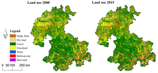
Figure 3.
Land use map in 2000 and 2015.
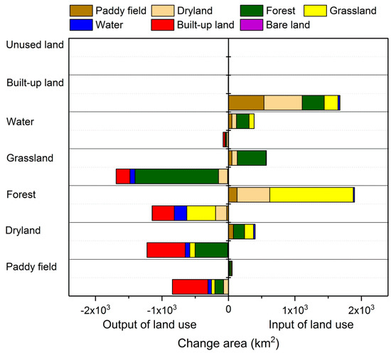
Figure 4.
Conversion between multiple land uses from 2000 to 2015.
Considerable farmlands were occupied by the expansion of built-up lands, and also conversed to the forest under the Grain for Green Project [60]. Meanwhile, forests and grasslands were reclaimed to the farmlands under the Requisition-compensation Balance Policy of Farmland [61], where the majority of land was reclaimed to dry land, but few to paddy field. The most intense conversion was between forest and grassland. With the ecological restoration project, the forest area significantly increased from the grassland (major source) and farmland, while several forested lands degraded to grassland. The built-up land significantly expanded with a higher change rate of 63.49% than those of others, at the expense of farmland (major source), forest, and grassland. The conversion area of water and bare land is relatively small, where the farmland, forest, and grassland were restored to water while small amounts of bare lands were developed.
The correlations of the driving factors to land uses were analyzed by the logistic regression model (Table 5). Using the coefficients of driving factors at the significant level of 0.05 to build the modified logistic regression model by the Equation (8), the ROC values evaluated the model fitness between land uses and driving data. The spatial pattern of forest, paddy field, dry land and grassland can be reasonably explained by the independent variables with the high ROC values. The model fitness of built-up land and bare land show a relative poor fitness with relative lower ROC values. Almost different categories of factors would significantly influence the spatial distribution of the paddy field, dry land, forest, and grassland. The quantity of significant drivers at 0.05 level were 10, 10, 10, 11 for, respectively. In contrast, the quantity of significant drivers for the water, built-up land, and bare land were 6, 7, and 4. Climatic, topographic factors, GDP, and locations of rivers were important determinants of the distribution of water. Topographic factors socio-economic and location factors closely related to the built-up land.
Table 5.
Logistic regression model estimates for land use patterns.
3.2. Elevation-Based Stratification
With different scale parameter settings, the multi-segmentation based on the elevation was performed and the stratifications at the corresponding scale parameter were generated. Figure 5 shows the examples of the stratification results at four specific scale parameters. When the scale parameter equals 10,000, the segmentation divided the study area into different stratifications with an obvious elevation gradient from the northwest to southeast. A smaller scale parameter resulted in a larger number of stratifications, which depicted more details in the local terrain variations.
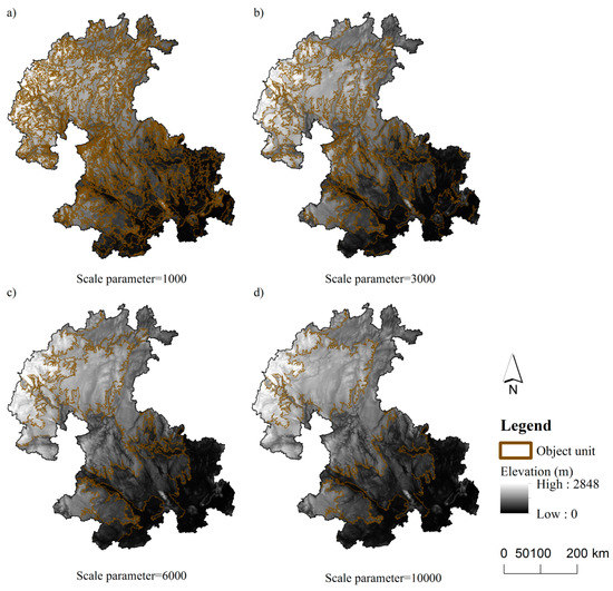
Figure 5.
Elevation-based stratifications at the scale parameter of (a) 1000; (b) 3000; (c) 6000; (d) 10,000.
Based on the land-use characteristics within the stratifications at different scale parameters, the ASDintra, LVinter, and OSS were calculated (Figure 6). The results showed a similar decrease in ASDintra and LVinter, but a more fluctuating change for LVinter. With the increase in the scale parameter, the ASDintra showed an initial significant decrease followed by a slow decrease. There was a somewhat fluctuating decrease of LVinter as the scale parameter increased. This change indicated an increase in intra-segment homogeneity, but a decrease in inter-segment heterogeneity as the scale parameter increased. This result implied that the maximization of the intra-segment homogeneity and inter-segment heterogeneity could not be realized simultaneously.
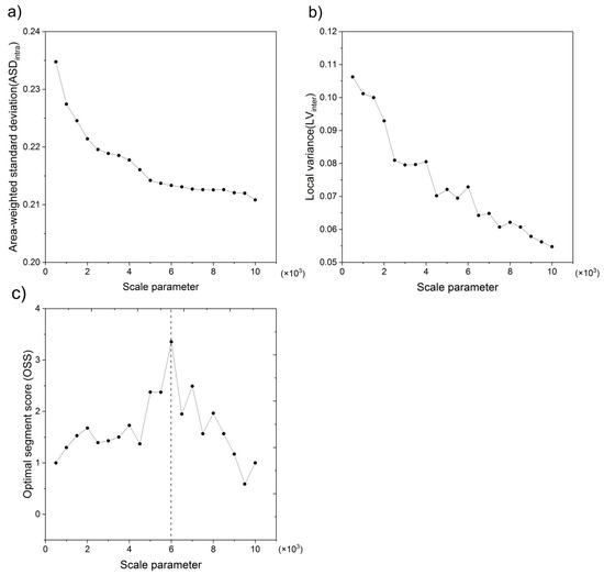
Figure 6.
Parameter determination for (a) area-weighted standard deviation of each stratification (ASDintra); (b) mean standard deviation of the stratifications (LVinter); (c) optimal segment score (OSS) as a function of scale parameter. Setting in eCognition software: Shape = 0.1, compactness = 0.5.
With the shape and compactness parameters of 0.1 and 0.5, the scale parameter was assigned with a step size of 500 and a range of 0–10,000 for eCognition software producing the stratifications (Figure 6). Taking these two objectives into consideration, the OSS was used to identify an optimal segmentation. The OSS showed an initial increase followed by a decrease with an increase in the scale parameter. Here, the OSS reached the maximum at the scale parameter of 6000, where the number of stratifications was eighteen for the model execution (Figure 5c). The average, minimum, and maximum value of area in the stratifications were 11,744, 2856 and 29,374 km2, respectively. Then, seventeen dummy variables for labeling the stratifications were added to the construction of the logistic regression model. The eighteen stratifications presented an elevation gradient pattern from northwest with the highest average elevation of 1732 m to southeast with the lowest average elevation of 144 m. The model showed that the area proportions of land-use types were significantly different within 18 stratifications (Figure 7). For example, the highest area proportion of built-up land was 6.37% in the stratification of the low elevation, including the province capital of Guangxi. In contrast, the area proportions of built-up land were lower than 0.1% in the stratification of the high elevation in the northwest of the study area. This stratification result was supposed to the optimal segmentation size and used as the basic boundary for the execution of SLUCS model.
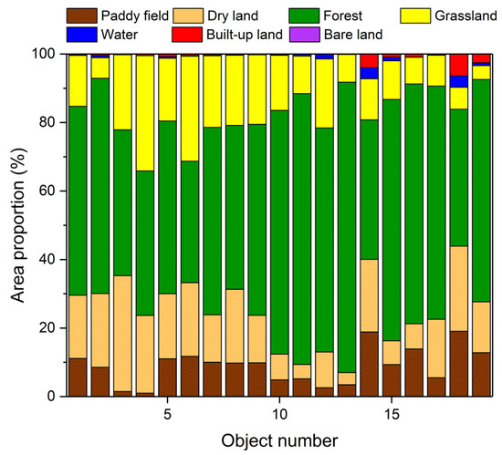
Figure 7.
Land use structure within stratifications at the optimal segmentation size.
3.3. Accuracy Assessment of SLUCS Model
To assess the accuracy, the simulated land use map in 2015 was projected by the SLUCS model and was compared to the referenced land use map from the visual interpretation in 2015 (Figure 8). The non-spatial land-use demand module used the same land-use changes demand from 2000 to 2015 as the actual interpreted land-use change in this period to execute the model. Based on the stratification result (Figure 5c), the stratified land-use demands, the stratified relationship between the land use and driving factors were calculated and the spatial allocation of the land-use were performed. Unlike the stratified method dividing the study area as several stratifications in the SLUCS, the traditional method, using the entire study area as the only one stratification, was used to simulate the land use with the same land-use demand.
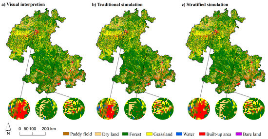
Figure 8.
Comparison of land use in 2015 from (a) referenced visual interpretation; (b) traditional simulation; (c) stratified simulation.
Based on the visual comparison in the whole study area and three enlarged sample windows, the referenced and simulated land-use maps were similar in many aspects. Especially, the performance of SLUCS model on the land-use change was examined. As a main land-use conversion type, the expansion of built-up land significantly modified the earth surface, increased the impervious surface area and became the focus of attention. The first sample window was in the Guiyang (province capital of Guizhou Province) and experienced a rapid and large-scale of built-up land expansion. Except for the tiny built-up land expansion, a good degree of spatial consistency between the stratified simulation and referenced result was found, while there was a relative spatial disparity between the traditional simulation and the reference in this window. The traditional method presented a relatively increased spatial dispersion distribution of built-up land compared to the reference. The forest covered over 50% of the total area, and its expansions, sourcing from the farmland and grassland, were examined in the second and third sample windows, respectively. The windows showed that both the traditional and stratified simulation presented a globally spatial fit, but a local disparity with the referenced land-use map. The results presented a more continuous patch than the referenced result by eliminating several small patches of these land-use types. Especially, the traditional method result showed a larger magnitude of patch eliminating, which would lead to a bias in the simulation result.
The kappa coefficient, KSimulation, and Modified Lee and Sallee metric were calculated to assess the accuracy (Table 6). The kappa coefficients of the traditional and stratified simulation were 0.83 and 0.89, respectively. This validated a globally quality performance of the models and a relatively better performance of stratified simulation results. With the conversion resistance, the model can perform well with the persistence in land use located in areas without land use changes [18]. As only 2.4% of locations changed from 2000 to 2015, other areas without land use changes in this period would present a good spatial consistence between referenced and simulated results. The KSimulation showed a much higher value of the stratified simulation (0.52) than that of the traditional simulation (0.19), indicating a much better performance of the stratified simulation on regions occurring land use changes from 2000 to 2015. Comparing the spatial fitness of each land-use type, the Modified Lee and Sallee metrics of paddy field, dry land, forest, and grassland were larger than 0.90 for both of two simulation methods, presenting a much higher degree of spatial fit. In contrast, the stratified method presented a better simulating performance for the water and built-up land than the traditional method.
Table 6.
Accuracy assessment of land use change simulation.
3.4. Simulation of Land-Use Change in 2030
Based on the three scenario settings, the spatial land uses of the study area in 2030 were projected (Figure 9 and Table 7). Consistent with the change in the trend from 2000 to 2015, three scenarios presented the same change in trends, but with different magnitudes for each land-use type from 2015 to 2030. The forest, water, and built-up land increased, while inversely the paddy field, dry land, grassland, and bare land decreased. The historic-condition scenario presented a relatively low change rate of land use, while the planning and protect scenarios forecasted a sharp increase of built-up land and forest, respectively, but a sharp decrease of other land-use types.
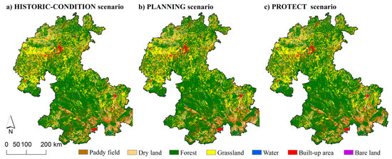
Figure 9.
Projection of land use 2015 under the (a) history trend scenario (historic-condition); (b) socioeconomic priority scenario (planning); (c) Ecological protection scenario (protect).
Table 7.
Change of land use from 2015 to 2030 under different scenarios.
The change rate of the built-up land was still the highest for the historic-condition, planning and protect scenarios, with values of 36.6%, 40.4%, and 30.2%, respectively. Not only an expansion of built-up land was found surrounding the metropolis, but also was located in several towns with the scattered distribution. Specially, the cities of Guiyang, Zunyi, Nanning, and Liuzhou experienced a large area of built-up land expansion from 2000 to 2015 and continuously increased in area in the future simulation. The increase of forest was small with the change rate of 0.7% in the historic-condition scenario, but were significantly enlarged as the largest area of all land-use types to 2.8% and 5.5% in the planning and protect scenarios, respectively. Areas of new afforestation tended to converse from the scattered distribution grassland (the main source) and farmland, which was mainly located surrounding the formerly existing forests in relatively high elevations. The planning scenario showed the lowest increase of water, while that of the protect scenario was the highest.
For the two types of farmlands, the paddy field had a higher decreased rate than the dry land in the three scenarios, due to a larger proportion of built-up land occupation for the paddy field. The decreased rate of farmland enlarged in turn for the historic-condition, planning, and protect scenarios. Also, the decreased magnitude of grassland showed a similar change in trend among these three scenarios. Particularly, the decreased rate of grassland in planning and protect had enlarged to 10.1% and 14.5%, respectively. These three types of land use became the major sources of other land use. The area of bare land is tiny and only a few of them were developed to other land uses.
4. Discussion
The novelty of our established SLUCS model is that it uses the strategy of elevation-based stratification to get a better approximation for the land use dynamics process. Elevation gradients reflects the differences in meteorological variables, soil properties, and vegetative functions [20,21], and further influences the functional orientation of land use, as well as the activities and human demands on the land use [19,22]. Along the elevation-based stratifications, the model used the quantitative method to better quantify stratified land-use demands and the stratified relationship of driving factors to land use to improve model performance. Not unlike the method of subjective division used in previous studies [16,18], the elevation-based stratification module of the SLUCS model developed a quantitative method of dividing the study area into multiple stratifications. Based on the proposed ASDintra, LVinter, and OSS in this study, the intra-segment homogeneity and the inter-segment heterogeneity of the land-use characteristics within different elevation gradients were comprehensively taken into consideration to perform the segmentation and generate stratifications at the optimal segmentation size.
The elevation-based strategy produced stratifications along the elevation gradients relating to different spatial patterns of physical and social-economic factors, which can better present the spatial land use characteristics and simulate the land use change. Stratifications can ensure that region-level results from macro-scale models are spatially allocated [18]. Comparing to the administrative unit with the fixed boundaries, the SLUCS model flexibly divided the entire study area to multiple stratifications based on the elevation and land use characteristics. The municipal boundaries consisting of sixteen units (Figure S2) was used to calculate the inter-segment heterogeneity of land use in 2000 (LVinter). LVinter of municipal boundaries is 0.048, which is nearly less than one third of that for elevation-based stratifications of our model (0.074). It indicated a larger spatial variation of land use characteristics for the elevation-based stratifications than that of municipal boundaries. Within different stratifications from the elevation-based stratification module, the land-use characteristics and historical changes were different from each other, indicating the spatial difference of land utilization orientation (Figure 7). For example, the two stratifications with the high elevations of 1732 m and 1714 m located in the northwest of the study area would have a higher increased rate of forests of 3.02% and 2.75%, which are much higher than the average value of 0.60% in the entire study area. In contrast, the stratification with the lowest average elevation of 144 m located in the southwest had the highest built-up land area proportion of 6.37% in 2000 and presented the highest increase area of 486 km2 from 2000 to 2015. Thus, the non-spatial land-use demand module would better present the spatial differences in land-use actives within the elevation gradients, forecast stratified land-use demand, and set zoning constraints for simulating land use [62]. Better quantifying the relationship of the driving factors with land use would significantly help improve the simulation accuracy of the land-use change [46,63]. Using the dummy variables to indicate different stratifications in the logistic regression model, the stratified analysis could reveal the regional differences in the impacts of the driving factors on land use [12]. The stratified suitability estimation can provide new spatial information regarding land-use change to improve model performance.
The application of the SLUCS model in the study area validated its effectiveness to project land-use change (Figure 8 and Table 6). Compared to the traditional method, without the stratifications, the stratification strategy of the SLUCS model exhibited superior spatial consistency with the reference land use (from the visualized interpretation) and higher accuracy assessment (from the statistical metrics). Previous studies validated the idea that the traditional method could account for land-use persistence simulated the area without land use change in the simulation period well [18,35,58]. As only 2.4% of the reported locations changed from 2000 to 2015, both presented a high kappa coefficient. However, the high KSimulation indicated the much better performance in simulated areas experiencing land-use conversion when the stratified method was used than the traditional method [58]. In particular, the stratified method resulted in a better spatially visualized fit (Figure 8) with the reference and a higher Modified Lee and Sallee metric (Table 6) for simulating the built-up land expansion. The urban growth was constrained by stricter planning and management efforts in China within different administrative units [64]. Thus, there was a clear spatial gradient in the urbanization ratio and the urbanization gaps among different regions persisted [65]. The traditional method was not able to fully simulate the regional differences in the urbanization process and projected a spatial dispersion distribution of built-up land. In contrast, the stratified method had the advantage of a stratified consideration of the regional urbanization process and built-up land expansion. The improvement of SLUCS model in projecting land use change would provide a more reliable output to support for the decision making.
To a certain degree, our model had limitations and did not perform well in local areas of land-use conversion. The model showed that the simulation accuracies of the built-up land were still lower than other land-use types and presented a spatial disparity within the referenced land use in tiny conversion areas. Comparing to ROC values of around 0.85 in previous studies of predicting urban growth [66,67], the ROC of 0.78 is relative lower in the logistic model for built-up land. This indicated that the model cannot fully explain the spatial variability of built-up land and would further influence the local performance of the model simulation. Land use change is determined by the interaction of driving factors, where different spatial resolutions of data would affect the simulated results and may cause uncertainties. The aggregated data at coarse scales may obscure the local variability, but can show patterns invisible at fine scales, and vice versa [68]. Different biophysical and socio-economic processes influence the land use at their own dominant scale [69], but there is not an absolutely optimal scale for the system [70]. The data source determined the basic analysis pixel size [68]. As the spatial resolution in most of driving factors is 1000 × 1000 m, other factors were resampled at the same pixel size. Incorporation of the fine-scale socio-economic process is difficult, due to the high data requirements at this scale. Quantification of the land-use planning and policy, significantly influencing the built-up land expansion, was difficult even with detailed spatial information [71]. Thus, this study could only characterize the different macro-scale land-use demands driven by the land-use policy and planning within different stratifications. Also, there were difficulties in determining a straightforward quantitative approach for human demands and activities on land [72,73]. The use of several proxies for them in this study (Table 1), which have proven to be acceptable in recent studies, would influence the local performance of the model. As only seven independent variables at the significant level of 0.05 were used to build the logistic model, the spatial-explicitly detailed socio-economic factors would help improve the model performance in the future study.
In addition, this study hypothesized that the optimal segmentation was identified as the one with the highest OSS, and seventeen dummy variables were added into the regression model. With more independent variables, there may be statistical uncertainty for the estimation with additional parameters [74]. The application of SLUCS model in the other study areas could be tested to produce a reasonable number of stratifications and validate the performance of the stratified strategy, where the number is not too large or small. Also, this study only used the elevation data to perform the segmentation to examine the effect of the elevation gradient on the land use. Other features could be selected and tested to generate the stratification with multiple environmental variables [26,27]. Considering the data availability, only temporal scales of partial driving factors with obviously changes from 2000 to 2015 were updated to simulate the land use in 2030 (Figure 9). Other factors with gradual and minor changes can be updated in the future study to better project the land use.
The SLUCS model can project the spatial pattern of future land use change under different land use scenarios. With multiple demands in terms of economic development, food security, and ecological protection, frequent conflict and competition occurs between multiple land-use types [75]. Under the three scenarios, the outputs of the SLUCS model demonstrated the potential land-use change and competition with different land-use priorities and strategies. Consistent for most regions in China [76], the model indicated an increasing threat to food security in the future with a continuing decline in farmlands in all the scenarios; this crisis will raise the priority on socio-economic growth and ecological protection in the planning and protect scenarios. The planning scenario presented a more scattered pattern of built-up land, with the largest increased area of built-up land under the three scenarios. This scenario implied that the limited flat land resources in the mountainous areas would restrict the expansion of built-up land near cities and part of the future built-up land will have to be dispersed. Over-urbanization in the mountains may easily damage the ecosystem [77] and calls for the scientific planning of urbanization in the study area [78]. The protect scenario showed that a significant increase in forests could be realized at the huge expense of low increase rate of built-up land and high decrease rate of farmlands and grasslands. Investments into ecological protection and willingness to make socio-economic sacrifices should be taken into consideration during decision making [79,80].
Limited land resources suitable for living and production in the karst mountain region would accelerate the different demands for land-use activities [31]. The tradeoffs among the different land-use types were suggested to support land-use planning and management. Our model visualized the land system dynamic process and projected the land-use change trajectory at the spatial dimension. With different target land-use scenarios, areas of land-use conversion can be identified using our model, which can then be used to evaluate their potential impacts, such as food production, soil conservation, water conservation, and biodiversity protection [2,9,81,82]. The conversion areas with high values of land-use should be the focus of land-use planning. For example, strict farmland protection policies should be implemented in the high production of farmlands occupied by built-up land, as per the model [83]. Comparing the three scenarios, areas of conversion from other land-use types to forests could be the priority of afforestation, because of the high suitability for forest planting. To coordinate multiple conflicting land-use types, information regarding different land-use change trajectories could provide potential options for sustainable land use.
5. Conclusions
Better understanding and projecting of land system dynamics will support the design and implementation of land-use planning and policy. To quantify the regional differences in land-use changes within the elevation gradient, this study built a novel SLUCS model using the elevation-based stratification strategy. Along the elevation gradients, the stratifications can make zoning constraints for the simulation with different land utilization orientations and quantify the stratified relationship of the driving factors with land uses, which help better approximate the land use dynamics process. The model included four modules: Elevation-based stratification, non-spatial land-use demand, stratified suitability estimation, and spatial allocation of land use. The first module developed a quantitative method of generating stratifications at the optimal segmentation size using ASDintra, LVinter, and OSS, which considered the intra-segment homogeneity and inter-segment heterogeneity of land-use characteristics. The second module presented the regional demands for land use and made zoning constraints for simulating land use. The third module utilized the stratified logistic regression model, with dummy variables to indicate different stratifications in order to reveal the regional differences in the relationship between driving factors and land use. Taking the Guizhou and Guangxi Karst Mountainous Region as the case study area, the model was executed to validate its performance. The effectiveness of the SLUCS model for projecting land-use change was validated. Compared to the traditional method without stratifications, the stratification strategy demonstrated an improved model performance than the traditional method, including a better spatial consistency with the reference and a higher accuracy assessment. Particularly, a much better model performance of simulating land use conversion areas was seen in the SLUCS model, where the KSimulation was higher (0.52) than that of the traditional model (0.19). Further, a better built-up land expansion simulation accuracy was seen, based on the Modified Lee and Sallee metric. The historic-condition, planning and protect scenarios from 2015 to 2030 were designed with different land-use priorities and management strategies. Under the three scenarios, the outputs of the SLUCS model projected the potential land-use changes and visualized the competition between different land uses. Consistent with the historical change trend from 2000 to 2015, the three scenarios presented the same change trends, but with different magnitudes. The HISTROY scenario forecasted the historical trend of land use according to the change in the past 15 years. The planning scenario presented the highest increase in built-up land among three scenarios from conversions of a large area of paddy field, dry land, and grassland. The protect scenario presented the highest increase in forests at the expense of low increase in built-up land and high decrease in farmland and grassland. Various management and tradeoff strategies for the multiple land-use types were suggested, based on the different scenarios. The results validated the effectiveness of the SLUCS model and the significance of supporting sustainable land use. The limitations and possible improvements of the SLUCS model mentioned in this paper can be tested in future research, including the data acquisition of spatial-explicitly detailed socio-economic factors for better explaining land use patterns and improvement of the stratification producing process with the optimal segmentation and multiple environmental variables.
Supplementary Materials
The following are available online at http://www.mdpi.com/2072-4292/10/11/1730/s1, Table S1: Land use transition probability matrix of under Markov hypothesis from 2000 to 2015, Figure S1: Location of natural reserves in the Guizhou and Guangxi Karst Mountainous Region, Figure S2: Municipal boundary in the Guizhou and Guangxi Karst Mountainous Region.
Author Contributions
E.X. and H.Z. conceived and designed the experiments. E.X. and L.Y. analyzed the data. E.X. and H.Z. wrote and revised the paper.
Funding
This work was financially by National Natural Science Foundation of China (Grant No. 41601095), Strategic Priority Research Program of the Chinese Academy of Sciences (XDA19040305) and National Basic Research Program of China (973 Program) (2015CB452702).
Conflicts of Interest
The authors declare no conflict of interest.
References
- Vitousek, P.M.; Mooney, H.A.; Lubchenco, J.; Melillo, J.M. Human domination of Earth’s ecosystems. Science 1997, 277, 494–499. [Google Scholar] [CrossRef]
- Foley, J.A.; DeFries, R.; Asner, G.P.; Barford, C.; Bonan, G.; Carpenter, S.R.; Chapin, F.S.; Coe, M.T.; Daily, G.C.; Gibbs, H.K. Global consequences of land use. Science 2005, 309, 570–574. [Google Scholar] [CrossRef] [PubMed]
- Lambin, E.F.; Meyfroidt, P. Global land use change, economic globalization, and the looming land scarcity. Proc. Natl. Acad. Sci. USA 2011, 108, 3465–3472. [Google Scholar] [CrossRef] [PubMed]
- Tilman, D.; Balzer, C.; Hill, J.; Befort, B.L. Global food demand and the sustainable intensification of agriculture. Proc. Natl. Acad. Sci. USA 2011, 108, 20260–20264. [Google Scholar] [CrossRef] [PubMed]
- Seto, K.C.; Fragkias, M.; Güneralp, B.; Reilly, M.K. A Meta-Analysis of Global Urban Land Expansion. PLoS ONE 2011, 6, e23777. [Google Scholar] [CrossRef] [PubMed]
- Trabucco, A.; Zomer, R.J.; Bossio, D.A.; van Straaten, O.; Verchot, L.V. Climate change mitigation through afforestation/reforestation: A global analysis of hydrologic impacts with four case studies. Agric. Ecosyst. Environ. 2008, 126, 81–97. [Google Scholar] [CrossRef]
- Bryan, B.A.; Gao, L.; Ye, Y.; Sun, X.; Connor, J.D.; Crossman, N.D.; Stafford-Smith, M.; Wu, J.; He, C.; Yu, D.; et al. China’s response to a national land-system sustainability emergency. Nature 2018, 559, 193–204. [Google Scholar] [CrossRef] [PubMed]
- Kalnay, E.; Cai, M. Impact of urbanization and land-use change on climate. Nature 2003, 423, 528–531. [Google Scholar] [CrossRef] [PubMed]
- Lambin, E.F.; Turner, B.L.; Geist, H.J.; Agbola, S.B.; Angelsen, A.; Bruce, J.W.; Coomes, O.T.; Dirzo, R.; Fischer, G.; Folke, C. The causes of land-use and land-cover change: Moving beyond the myths. Glob. Environ. Chang. 2001, 11, 261–269. [Google Scholar] [CrossRef]
- Verburg, P.H.; Schot, P.P.; Dijst, M.J.; Veldkamp, A. Land use change modelling: Current practice and research priorities. GeoJournal 2004, 61, 309–324. [Google Scholar] [CrossRef]
- Van Schrojenstein Lantman, J.; Verburg, P.H.; Bregt, A.; Geertman, S. Core principles and concepts in land-use modelling: A literature review. In Land-Use Modelling in Planning Practice; Springer: Dordrecht, The Netherlands, 2011; pp. 35–57. [Google Scholar]
- Santé, I.; García, A.M.; Miranda, D.; Crecente, R. Cellular automata models for the simulation of real-world urban processes: A review and analysis. Landsc. Urban Plan. 2010, 96, 108–122. [Google Scholar] [CrossRef]
- De Rosa, M.; Knudsen, M.T.; Hermansen, J.E. A comparison of Land Use Change models: Challenges and future developments. J. Clean. Prod. 2016, 113, 183–193. [Google Scholar] [CrossRef]
- Brown, D.G.; Verburg, P.H.; Pontius, R.G.; Lange, M.D. Opportunities to improve impact, integration, and evaluation of land change models. Curr. Opin. Environ. Sustain. 2013, 5, 452–457. [Google Scholar] [CrossRef]
- Matthews, R.B.; Gilbert, N.G.; Roach, A.; Polhill, J.G.; Gotts, N.M. Agent-based land-use models: A review of applications. Landsc. Ecol. 2007, 22, 1447–1459. [Google Scholar] [CrossRef]
- Van Asselen, S.; Verburg, P.H. A Land System representation for global assessments and land-use modeling. Glob. Chang. Biol. 2012, 18, 3125–3148. [Google Scholar] [CrossRef] [PubMed]
- Kroll, F.; Müller, F.; Haase, D.; Fohrer, N. Rural-urban gradient analysis of ecosystem services supply and demand dynamics. Land Use Policy 2012, 29, 521–535. [Google Scholar] [CrossRef]
- Van Asselen, S.; Verburg, P.H. Land cover change or land-use intensification: Simulating land system change with a global-scale land change model. Glob. Chang. Biol. 2013, 19, 3648–3667. [Google Scholar] [CrossRef] [PubMed]
- Tovar, C.; Seijmonsbergen, A.C.; Duivenvoorden, J.F. Monitoring land use and land cover change in mountain regions: An example in the Jalca grasslands of the Peruvian Andes. Landsc. Urban Plan. 2013, 112, 40–49. [Google Scholar] [CrossRef]
- Lemenih, M.; Itanna, F. Soil carbon stocks and turnovers in various vegetation types and arable lands along an elevation gradient in southern Ethiopia. Geoderma 2004, 123, 177–188. [Google Scholar] [CrossRef]
- Zhang, Y.; Wilmking, M. Divergent growth responses and increasing temperature limitation of Qinghai spruce growth along an elevation gradient at the northeast Tibet Plateau. For. Ecol. Manag. 2010, 260, 1076–1082. [Google Scholar] [CrossRef]
- Becker, A.; Körner, C.; Brun, J.-J.; Guisan, A.; Tappeiner, U. Ecological and Land Use Studies along Elevational Gradients. Mt. Res. Dev. 2007, 27, 58–65. [Google Scholar] [CrossRef]
- Chen, C.-F.; Son, N.-T.; Chang, N.-B.; Chen, C.-R.; Chang, L.-Y.; Valdez, M.; Centeno, G.; Thompson, C.; Aceituno, J. Multi-Decadal Mangrove Forest Change Detection and Prediction in Honduras, Central America, with Landsat Imagery and a Markov Chain Model. Remote Sens. 2013, 5, 6408–6426. [Google Scholar] [CrossRef]
- Jongman, R.; Bunce, R.; Metzger, M.; Mücher, C.; Howard, D.; Mateus, V. Objectives and applications of a statistical environmental stratification of Europe. Landsc. Ecol. 2006, 21, 409–419. [Google Scholar] [CrossRef]
- Metzger, M.; Rounsevell, M.; Acosta-Michlik, L.; Leemans, R.; Schröter, D. The vulnerability of ecosystem services to land use change. Agric. Ecosyst. Environ. 2006, 114, 69–85. [Google Scholar] [CrossRef]
- Zomer, R.J.; Trabucco, A.; Wang, M.; Lang, R.; Chen, H.; Metzger, M.J.; Smajgl, A.; Beckschäfer, P.; Xu, J. Environmental stratification to model climate change impacts on biodiversity and rubber production in Xishuangbanna, Yunnan, China. Biol. Conserv. 2014, 170, 264–273. [Google Scholar] [CrossRef]
- Kieu, C.; Zhang, D.L. The Control of Environmental Stratification on the Hurricane Maximum Potential Intensity. Geophys. Res. Lett. 2018. [Google Scholar] [CrossRef]
- Blaschke, T.; Hay, G.J.; Kelly, M.; Lang, S.; Hofmann, P.; Addink, E.; Feitosa, R.Q.; Van der Meer, F.; Van der Werff, H.; Van Coillie, F. Geographic object-based image analysis—Towards a new paradigm. ISPRS J. Photogramm. Remote Sens. 2014, 87, 180–191. [Google Scholar] [CrossRef] [PubMed]
- Luo, G.; Yin, C.; Chen, X.; Xu, W.; Lu, L. Combining system dynamic model and CLUE-S model to improve land use scenario analyses at regional scale: A case study of Sangong watershed in Xinjiang, China. Ecol. Complex. 2010, 7, 198–207. [Google Scholar] [CrossRef]
- Waltham, T. Fengcong, fenglin, cone karst and tower karst. Cave Karst Sci. 2008, 35, 77–88. [Google Scholar]
- Xu, E.; Zhang, H. Vertical distribution of land use in karst mountainous region. Chin. J. Eco-Agric. 2016, 24, 1693–1702. (In Chinese) [Google Scholar]
- Shi, X.Z.; Yu, D.S.; Warner, E.D.; Sun, W.X.; Petersen, G.W.; Gong, Z.T.; Lin, H. Cross-Reference System for Translating Between Genetic Soil Classification of China and Soil Taxonomy. Soil Sci. Soc. Am. J. 2006, 70, 78–83. [Google Scholar] [CrossRef]
- Liu, J.; Liu, M.; Zhuang, D.; Zhang, Z.; Deng, X. Study on spatial pattern of land-use change in China during 1995–2000. Sci. China-Earth Sci. 2003, 46, 373–384. [Google Scholar]
- Huang, Q.-H.; Cai, Y.-L. Simulation of land use change using GIS-based stochastic model: The case study of Shiqian County, Southwestern China. Stoch. Environ. Res. Risk Assess. 2007, 21, 419–426. [Google Scholar] [CrossRef]
- Liu, Z.; Verburg, P.H.; Wu, J.; He, C. Understanding land system change through scenario-based simulations: A case study from the drylands in northern China. Environ. Manag. 2017, 59, 440–454. [Google Scholar] [CrossRef] [PubMed]
- Didan, K.; Munoz, A.B.; Solano, R.; Huete, A. MODIS Vegetation Index User’s Guide (MOD13 Series); Vegetation Index and Phenology Lab, University of Arizona: Tucson, AZ, USA, 2015. [Google Scholar]
- Xu, E.Q.; Zhang, H.Q. Characterization and interaction of driving factors in karst rocky desertification: A case study from Changshun, China. Solid Earth 2014, 5, 1329–1340. [Google Scholar] [CrossRef]
- Dong, G.; Xu, E.; Zhang, H. Spatiotemporal variation of driving forces for settlement expansion in different types of counties. Sustainability 2016, 8, 39. [Google Scholar] [CrossRef]
- Southworth, J.; Marsik, M.; Qiu, Y.; Perz, S.; Cumming, G.; Stevens, F.; Rocha, K.; Duchelle, A.; Barnes, G. Roads as Drivers of Change: Trajectories across the Tri-National Frontier in MAP, the Southwestern Amazon. Remote Sens. 2011, 3, 1047–1066. [Google Scholar] [CrossRef]
- Shangguan, W.; Dai, Y.J.; Liu, B.Y.; Ye, A.Z.; Yuan, H. A soil particle-size distribution dataset for regional land and climate modelling in China. Geoderma 2012, 171, 85–91. [Google Scholar] [CrossRef]
- Kim, M.; Madden, M.; Warner, T. Estimation of optimal image object size for the segmentation of forest stands with multispectral IKONOS imagery. In Object-Based Image Analysis; Springer: New York, NY, USA, 2008; pp. 291–307. [Google Scholar]
- Baatz, M.; Benz, U.; Dehghani, S.; Heynen, M.; Höltje, A.; Hofmann, P.; Lingenfelder, I.; Mimler, M.; Sohlbach, M.; Weber, M. eCognition User Guide; Definiens Imaging: Munich, Germany, 2004. [Google Scholar]
- Gilks, W.R.; Richardson, S.; Spiegelhalter, D. Markov Chain Monte Carlo in Practice; Chapman & Hall: London, UK, 1995. [Google Scholar]
- Liao, J.; Tang, L.; Shao, G.; Su, X.; Chen, D.; Xu, T. Incorporation of extended neighborhood mechanisms and its impact on urban land-use cellular automata simulations. Environ. Model. Softw. 2016, 75, 163–175. [Google Scholar] [CrossRef]
- Harrell, F.E. Regression modeling strategies. In Ordinal Logistic Regression; Springer: New York, NY, USA, 2015; pp. 311–325. [Google Scholar]
- Verburg, P.H.; Soepboer, W.; Veldkamp, A.; Limpiada, R.; Espaldon, V.; Mastura, S.S. Modeling the spatial dynamics of regional land use: The CLUE-S model. Environ. Manag. 2002, 30, 391–405. [Google Scholar] [CrossRef] [PubMed]
- De Almeida Furtado, L.F.; Silva, T.S.F.; de Moraes Novo, E.M.L. Dual-season and full-polarimetric C band SAR assessment for vegetation mapping in the Amazon várzea wetlands. Remote Sens. Environ. 2016, 174, 212–222. [Google Scholar] [CrossRef]
- Li, X.; Myint, S.W.; Zhang, Y.; Galletti, C.; Zhang, X.; Turner, B.L. Object-based land-cover classification for metropolitan Phoenix, Arizona, using aerial photography. Int. J. Appl. Earth Obs. Geoinf. 2014, 33, 321–330. [Google Scholar] [CrossRef]
- Myint, S.W.; Galletti, C.S.; Kaplan, S.; Kim, W.K. Object vs. pixel: A systematic evaluation in urban environments. Geocarto Int. 2013, 28, 657–678. [Google Scholar] [CrossRef]
- Platt, R.V.; Rapoza, L. An evaluation of an object-oriented paradigm for land use/land cover classification. Prof. Geogr. 2008, 60, 87–100. [Google Scholar] [CrossRef]
- Johnson, B.; Xie, Z. Unsupervised image segmentation evaluation and refinement using a multi-scale approach. ISPRS J. Photogramm. Remote Sens. 2011, 66, 473–483. [Google Scholar] [CrossRef]
- Gabriel, K.R.; Neumann, J. A Markov chain model for daily rainfall occurrence at Tel Aviv. Q. J. R. Meteorol. Soc. 1962, 88, 90–95. [Google Scholar] [CrossRef]
- Hosmer, D.W., Jr.; Lemeshow, S.; Sturdivant, R.X. Applied Logistic Regression; John Wiley & Sons: New York, NY, USA, 2013; Volume 398. [Google Scholar]
- Sun, P.; Xu, Y.; Yu, Z.; Liu, Q.; Xie, B.; Liu, J. Scenario simulation and landscape pattern dynamic changes of land use in the Poverty Belt around Beijing and Tianjin: A case study of Zhangjiakou city, Hebei Province. J. Geogr. Sci. 2016, 26, 272–296. [Google Scholar] [CrossRef]
- Verburg, P.H.; van Eck, J.R.R.; de Nijs, T.C.M.; Dijst, M.J.; Schot, P. Determinants of Land-Use Change Patterns in the Netherlands. Environ. Plan. B Plan. Des. 2004, 31, 125–150. [Google Scholar] [CrossRef]
- Pontius, R.G.; Schneider, L.C. Land-cover change model validation by an ROC method for the Ipswich watershed, Massachusetts, USA. Agric. Ecosyst. Environ. 2001, 85, 239–248. [Google Scholar] [CrossRef]
- Congalton, R.G. A review of assessing the accuracy of classifications of remotely sensed data. Remote Sens. Environ. 1991, 37, 35–46. [Google Scholar] [CrossRef]
- Van Vliet, J.; Bregt, A.K.; Hagen-Zanker, A. Revisiting Kappa to account for change in the accuracy assessment of land-use change models. Ecol. Model. 2011, 222, 1367–1375. [Google Scholar] [CrossRef]
- Jantz, C.A.; Goetz, S.J.; Shelley, M.K. Using the SLEUTH urban growth model to simulate the impacts of future policy scenarios on urban land use in the Baltimore-Washington metropolitan area. Environ. Plan. B Plan. Des. 2004, 31, 251–271. [Google Scholar] [CrossRef]
- Chen, Y.; Wang, K.; Lin, Y.; Shi, W.; Song, Y.; He, X. Balancing green and grain trade. Nat. Geosci. 2015, 8, 739–741. [Google Scholar] [CrossRef]
- Liu, Y.; Fang, F.; Li, Y. Key issues of land use in China and implications for policy making. Land Use Policy 2014, 40, 6–12. [Google Scholar] [CrossRef]
- Li, X.; Yeh, A.G.O. Neural-network-based cellular automata for simulating multiple land use changes using GIS. Int. J. Geogr. Inf. Sci. 2002, 16, 323–343. [Google Scholar] [CrossRef]
- Veldkamp, A.; Lambin, E.F. Predicting land-use change. Agric. Ecosyst. Environ. 2001, 85, 1–6. [Google Scholar] [CrossRef]
- Deng, J.S.; Wang, K.; Hong, Y.; Qi, J.G. Spatio-temporal dynamics and evolution of land use change and landscape pattern in response to rapid urbanization. Landsc. Urban Plan. 2009, 92, 187–198. [Google Scholar] [CrossRef]
- Liu, J.; Zhang, Q.; Hu, Y. Regional differences of China’s urban expansion from late 20th to early 21st century based on remote sensing information. Chin. Geogr. Sci. 2012, 22, 1–14. [Google Scholar] [CrossRef]
- Vermeiren, K.; Van Rompaey, A.; Loopmans, M.; Serwajja, E.; Mukwaya, P. Urban growth of Kampala, Uganda: Pattern analysis and scenario development. Landsc. Urban Plan. 2012, 106, 199–206. [Google Scholar] [CrossRef]
- Hu, Z.; Lo, C.P. Modeling urban growth in Atlanta using logistic regression. Comput. Environ. Urban Syst. 2007, 31, 667–688. [Google Scholar] [CrossRef]
- Veldkamp, A.; Verburg, P.H.; Kok, K.; de Koning, G.H.J.; Priess, J.; Bergsma, A.R. The Need for Scale Sensitive Approaches in Spatially Explicit Land Use Change Modeling. Environ. Model. Assess. 2001, 6, 111–121. [Google Scholar] [CrossRef]
- Serrano-Tovar, T.; Giampietro, M. Multi-scale integrated analysis of rural Laos: Studying metabolic patterns of land uses across different levels and scales. Land Use Policy 2014, 36, 155–170. [Google Scholar] [CrossRef]
- Jackson, H.B.; Fahrig, L. Are ecologists conducting research at the optimal scale? Glob. Ecol. Biogeogr. 2015, 24, 52–63. [Google Scholar] [CrossRef]
- Wu, Y.; Zhang, X.; Shen, L. The impact of urbanization policy on land use change: A scenario analysis. Cities 2011, 28, 147–159. [Google Scholar] [CrossRef]
- Wang, X.M.; Chen, F.H.; Dong, Z.B. The relative role of climatic and human factors in desertification in semiarid China. Glob. Environ. Chang. 2006, 16, 48–57. [Google Scholar] [CrossRef]
- Lauf, S.; Haase, D.; Hostert, P.; Lakes, T.; Kleinschmit, B. Uncovering land-use dynamics driven by human decision-making—A combined model approach using cellular automata and system dynamics. Environ. Model. Softw. 2012, 27–28, 71–82. [Google Scholar] [CrossRef]
- Liu, D.B. Uncertainty Theory; Springer: Berlin/Heidelberg, Germany, 2007; pp. 205–234. [Google Scholar]
- DeFries, R.S.; Foley, J.A.; Asner, G.P. Land-use choices: Balancing human needs and ecosystem function. Front. Ecol. Environ. 2004, 2, 249–257. [Google Scholar] [CrossRef]
- Wang, J.; Chen, Y.; Shao, X.; Zhang, Y.; Cao, Y. Land-use changes and policy dimension driving forces in China: Present, trend and future. Land Use Policy 2012, 29, 737–749. [Google Scholar] [CrossRef]
- Zhang, B.; Mo, S.; Tan, Y.; Xiao, F.; Wu, H. Urbanization and De-urbanization in Mountain Regions of China. Mt. Res. Dev. 2004, 24, 206–209. [Google Scholar]
- Wei, D.; Yiping, F.; Wei, T. The strategic effect and general directions of urbanization in mountain areas of China. Bull. Chin. Acad. Sci. 2013, 28, 66–73. (In Chinese) [Google Scholar]
- Davis, J.L.; Le, B.; Coy, A.E. Building a model of commitment to the natural environment to predict ecological behavior and willingness to sacrifice. J. Environ. Psychol. 2011, 31, 257–265. [Google Scholar] [CrossRef]
- Xu, E.; Zhang, H.; Yang, Y.; Zhang, Y. Integrating a Spatially Explicit Tradeoff Analysis for Sustainable Land Use Optimal Allocation. Sustainability 2014, 6, 8909–8930. [Google Scholar] [CrossRef]
- Tscharntke, T.; Clough, Y.; Wanger, T.C.; Jackson, L.; Motzke, I.; Perfecto, I.; Vandermeer, J.; Whitbread, A. Global food security, biodiversity conservation and the future of agricultural intensification. Biol. Conserv. 2012, 151, 53–59. [Google Scholar] [CrossRef]
- Zhou, F.; Xu, Y.; Chen, Y.; Xu, C.Y.; Gao, Y.; Du, J. Hydrological response to urbanization at different spatio-temporal scales simulated by coupling of CLUE-S and the SWAT model in the Yangtze River Delta region. J. Hydrol. 2013, 485, 113–125. [Google Scholar] [CrossRef]
- Lichtenberg, E.; Ding, C. Assessing farmland protection policy in China. Land Use Policy 2008, 25, 59–68. [Google Scholar] [CrossRef]
© 2018 by the authors. Licensee MDPI, Basel, Switzerland. This article is an open access article distributed under the terms and conditions of the Creative Commons Attribution (CC BY) license (http://creativecommons.org/licenses/by/4.0/).