An Extension of Phase Correlation-Based Image Registration to Estimate Similarity Transform Using Multiple Polar Fourier Transform

Abstract

Image registration is a core technology of many different image processing areas and is widely used in the remote sensing community. The accuracy of image registration largely determines the effect of subsequent applications. In recent years, phase correlation-based image registration has drawn much attention because of its high accuracy and efficiency as well as its robustness to gray difference and even slight changes in content. Many researchers have reported that the phase correlation method can acquire a sub-pixel accuracy of $1/10$ or even $1/100$. However, its performance is acquired only in the case of translation, which limits the scope of the application of the method. However, there are few reports on the estimation of scales and angles based on the phase correlation method. To take advantage of the high accuracy property and other merits of phase correlation-based image registration and extend it to estimate the similarity transform, we proposed a novel algorithm, the Multilayer Polar Fourier Transform (MPFT), which uses a fast and accurate polar Fourier transform with different scaling factors to calculate the log-polar Fourier transform. The structure of the polar grids of MPFT is more similar to the one of the log-polar grid. In particular, for rotation estimation only, the polar grid of MPFT is the calculation grid. To validate its effectiveness and high accuracy in estimating angles and scales, both qualitative and quantitative experiments were carried out. The quantitative experiments included a numerical simulation as well as synthetic and real data experiments. The experimental results showed that the proposed method, MPFT, performs better than the existing phase correlation-based similarity transform estimation methods, the Pseudo-polar Fourier Transform (PPFT) and the Multilayer Fractional Fourier Transform method (MLFFT), and the classical feature-based registration method, Scale-Invariant Feature Transform (SIFT), and its variant, ms-SIFT.

1. Introduction

Image registration is a fundamental and challenging task that is used in many different research areas such as remote sensing, medical imaging, computer vision and video processing [1,2,3,4]. Especially in the remote sensing community, the technology is widely used in many applications, such as mapping of various applications, change detection, image fusion, mosaicking, and earth surface dynamics monitoring [5,6,7,8,9]. The accuracy of registration determines the quality of the remote sensing application and analysis and even the success or failure of these applications. Fortunately, because of the stability of the satellite platform and geolocation tools, the affine transformation model is able to fit the local spatial deformations of remote sensing images with the help of the initial geometric model. In practical applications, one commonly used strategy for image registration is to construct multi-level pyramid images and divide these images into multiple tiles; this is known as patch-based image registration [6,10]. Specifically, for small patches, the distortion of remote sensing images can reasonably be approximated as the differences in scale, rotation, and translation—the similarity transformation. Therefore, accurate estimation of similarity transformation is a very important and fundamental task.

Although feature-based image registration methods such as the Scale-Invariant Feature Transform (SIFT) [11] are popular registration methods with advantages of robustness to scale and rotation, the invariance of SIFT may not always be maintained on the remote sensing images. Remote sensing images come from different sensors, have different resolutions and spectra, and they are more special than natural images. In some cases, the principle orientations of corresponding points are not consistent, even in the opposite direction, which results in false matching and registration failure [12]. In recent years, image registration based on phase correlation has drawn considerable attention due to its high accuracy and other merits, such as robustness to noise and illumination variation, low computation cost, ease of parallelizing and constant consumption of time, irrespective of the content of images and amount of translation. In the case of displacement only, it can acquire 1/10 or even 1/100-pixel accuracy [13,14,15], and a popular image co-registration-based phase correlation software was also developed [16]. However, it is only suited for displacement estimation.

In this paper, to take advantage of the phase correlation-based image registration algorithm and to estimate the similarity transform more accurately, we extend the phase correlation-based method to estimate the scale, rotation, and displacement simultaneously. Here, we propose a novel algorithm, the Multiple Layers Polar Fourier Transform (MPFT). Firstly, a proper log-polar grid is constructed. Secondly, a fast and accurate polar Fourier transform with multiple scaling factors is calculated. Thirdly, a cubic interpolation is carried out to calculate the log-polar Fourier transform. Qualitative and quantitative experiments show that the proposed MPFT is superior to the existing methods based on phase correlation (the Multilayer Fractional Fourier Transform, MLFT [17] and the Pseudo-polar Fourier Transform, PPFT [18]) as well as the algorithms based on features (SIFT and ms-SIFT [19]).

The rest of the paper is organized as follows: the background of remote sensing image registration is introduced in Section 2. An overview and description of the proposed method are detailed in Section 3. The analysis and experimental results are presented in Section 4. The discussion is given in Section 5 and the conclusions are drawn in Section 6.

2. Background

Remote sensing image registration is a prerequisite of subsequent applications such as image stitching, time series analysis, and change detection. According to a survey [2], image registration methods can be divided into two categories: area-based registration methods and feature-based registration methods.

2.1. Feature-Based Methods

Feature-based registration methods are the more mature and popular methods. They mainly consist of three steps: feature detection, feature description, and feature matching. Among the feature-based methods, the most classical algorithm is the scale-invariant feature transform (SIFT) [11]. However, in the remote sensing community, the direct application of SIFT faces many problems such as the low positional accuracy of feature points, the poor distribution of detected feature points in the spatial and scale spaces, the sensitivity of feature descriptors to non-linear radiation distortion, and so on. Recently, a series of improved algorithms emerged to solve these problems. To address the low positional accuracy of feature points, oriented least square matching (OLSM) was proposed to improve the positional accuracy of local affine features [20]. For feature descriptors, the adaptive binning scale-invariant feature transform (AB-SIFT) descriptor was proposed to enhance the robustness to local geometric distortions [21] and the histogram of orientated phase congruency (HOPC) descriptor was developed to address the nonlinear radiometric differences [22]. To address the poor distribution of detected features, novel score criteria for the feature points, a feature detection method based on phase congruency, and the uniform partitioning strategy were utilized to generate an adequate number of high-quality, uniformly-distributed point features in the spatial and scale spaces, such as UR-SIFT [23], UC-SIFT [24], and MMPC-Lap [25]. For feature matching, a support-line descriptor based on multiple adaptive binning gradient histograms was developed to filter out the outliers after the initial matching [26] to produce more high-precision correspondences.

2.2. Area-Based Methods

Area-based matching methods can be loosely grouped into three sub-categories: correlation-based methods, mutual information-based methods, and phase correlation-based methods. The correlation-based and mutual information-based methods process the original pixel values directly, so they are sensitive to change in the gray value and content. The phase correlation-based method calculates the phase difference in the frequency domain, which is robust to radiation changes and slight content changes. So, we mainly focused on the phase correlation-based methods. The estimation of similarity transformation based on phase correlation is usually done in two steps, namely the scale and angle are firstly estimated, and then, the displacement is estimated.

For the estimation of displacement only, there are two basic approaches. One is the identification of the coordinates of the main peak of the inverse Fourier transform of the normalized cross-power spectrum matrix. The other method involves determining the linear phase difference in the frequency domain. For the first category, the commonly used solutions are interpolation methods, such as 1D parabolic functions, sinc functions, modified sinc functions and Gaussian functions [27,28,29]. However, the disadvantages of the method are its sensitivity to noise and other errors. For the other category, the main theoretical basis is that the phase difference is linear with respect to displacement in the frequency domain. However, the frequency components are easily corrupted by image noise, variation in the image content, and other complex geometric and photometric distortions. So, the key aspect of the method is to determine the uncorrupted frequency. Some methods are focused on fitting a 2D plane through the origin of the frequency coordinates, for example, the least squares adjustment method which filters out the effects of noise and aliasing at high frequencies [30], the Quick Maximum Density Power Estimator (QMDPE) [31,32], and the maximum kernel density estimator [33]. Some methods are focused on determining the best rank-one approximation to the normalized cross-spectrum matrix, for example, singular value decomposition [34,35], minimization with respect to the Frobenius norm, the weighted residual matrix between the actual computation cross-spectrum and the ideal one [36], and low-rank matrix factorization with a mixture of Gaussians applied to the cross-spectrum matrix [37]. Considering that aliasing and noise are also two of many factors that can corrupt the sub-pixel accuracy of phase correlation-based image registration, and that avoiding inverse Fourier Transform can alleviate the side effects of aliasing and noise, the method of calculating the linear phase difference is the most popular [30].

In regard to scale and rotation estimation based on phase correlation, the core technology is to calculate the log-polar Fourier transform accurately and efficiently. Two approaches to calculate the log-polar Fourier transform exist. One is directly interpolating the 2D Fourier transform in the Cartesian coordinate to calculate the log-polar transform. The most representative work of this type is presented in [17,38]. This method can recover any rotation at a scale of up to 2. In 2003, Stone et al. proposed an appropriate filter window, weighted to the original image, which can reduce the alias caused by the rotation and recovery scales to 2.5 with any rotation [18]. The other method involves accurately and efficiently calculating the Fourier transform value of each point from a specific structure, and then interpolating the Fourier transform values of these points with the specific structure to approximate the log-polar Fourier transform value. In 2005, Keller et al. [39] proposed a Pseudo-polar FFT-based algorithm, which can significantly decrease the interpolation error produced when calculating the polar Fourier transform with the same complexity as the 2D FFT. The method involves the construction of a special grid, named the pseudo-polar grid, where equispaced angular lines are replaced by equisloped ones, and the computation speed is fast. The method can recover scales of up to 4. However, the pseudo-polar grid also performs poorly in terms of registering images because of its inability to approximate the log-polar Fourier transform. Later, in 2006, the pseudo-log-polar FFT was developed. It separates the whole plane into two parts, BH and BV (BH and BV are two subsets of points, as detailed in [40]). In the calculation of the Fourier transform values of points in the BH and BV point sets, an interpolation operation is also needed, which leads to underlying error. So, the pseudo-log-polar FFT still fails to reduce the interpolation error greatly. In 2009, a Multilayer Fractional Fourier Transform (MLFFT) approach was proposed in [41], which approximates the log-polar grid points by using multilayer Cartesian grids with different scaling factors. Compared to the pseudo-log-polar grid, the MLFFT-based registration method improves the accuracy of angle and scale estimation. However, an interpolation scheme is necessary, even for only polar Fourier transforms, and more interpolation errors also occur in the log-polar Fourier transform.

This paper aims to further reduce or eliminate the interpolation error in the calculation of the log-polar or polar Fourier transform, and to improve the estimation accuracy of the scale and angle. Here, a special grid is constructed. It is composed of multiple polar grids with different scaling factors. Furthermore, each polar Fourier transform can be calculated accurately and efficiently. Additionally, the scaling factors of polar grids can be simply determined by the histogram of radii of the points of the destination log-polar grid in the radial direction. Because of the accurate calculation of the og-polar grid Fourier transform, it can acquire a higher registration accuracy than the existing algorithms. In particular, for angle estimation, there is no interpolation error, which can significantly improve the accuracy of angle estimation.

3. Methodology

3.1. Math Theory of Image Registration Based on Phase Correlation

The basic principles of phase correlation-based image registration are the Fourier shift theorem and the log-polar transform, which states that the displacement of two images in spatial domain can be formulated as a phase difference in the frequency domain. By applying the log-polar transform, the scale and rotation angle are transformed into translations in the radial and angular directions. So, the scale and rotation estimations are reduced to a shift estimation operation. Currently, the phase correlation-based method can acquire a sub-pixel accuracy only in the case of displacement [27,28,29].

Suppose that $f_1(x,y)$ and $f_2(x,y)$ represent the coordinates of a pixel in a reference and sensed image, respectively. Additionally, they satisfy the following relationship:

$$f_2(x,y)=f_1(x-x_0,y-y_0)$$

(1)

where $x_0$, $y_0$ is the displacement in the column and row directions, respectively. Then, the following expression can be derived according to the Fourier shift theorem:

$${\mathcal{F}}_2({\omega }_x,{\omega }_y)={\mathcal{F}}_1({\omega }_x,{\omega }_y)exp\{-i({\omega }_x{x}_0+{\omega }_y{y}_0)\}$$

(2)

where ${\mathcal{F}}_1({\omega }_x,{\omega }_y)$, ${\mathcal{F}}_2({\omega }_x,{\omega }_y)$ is the corresponding Fourier transform of $f_1(x,y)$ and $f_2(x,y)$, respectively. ${\omega }_x$ and ${\omega }_y$ are radian frequencies ranging from $-\pi$ to $\pi$. The normalized cross-power spectrum matrix is denoted by

$$Q({\omega }_x,{\omega }_y)=\frac{{\mathcal{F}}_2({\omega }_x,{\omega }_y){\mathcal{F}}_1{({\omega }_x,{\omega }_y)}^{*}}{\left|{\mathcal{F}}_1({\omega }_x,{\omega }_y){\mathcal{F}}_2({\omega }_x,{\omega }_y)\right|}=exp\left\{-i({\omega }_x{x}_0+{\omega }_y{y}_0)\right\}$$

(3)

where * denotes the complex conjugate. The magnitude of $Q({\omega }_x,{\omega }_y)$ is normalized to 1 for any frequency component. It is, therefore, insensitive to gray variation and image content, which makes the phase correlation-based method more suitable for matching images acquired by different sensors or times.

In theory, the normalized cross-power matrix Q is a rank-one matrix, i.e., the phase difference is linear. As a result, Q is separable and can be expressed as the following equation:

$$Q({\omega }_x,{\omega }_y)=exp\left\{-i\left({\omega }_x{x}_0\right)\right\}exp\left\{(-i\left({\omega }_y{y}_0\right))\right\}=q_{x_0}\left({\omega }_x\right)q_{y_0}\left({\omega }_y\right).$$

(4)

After calculating the phase difference using the least squares fit or singular value decomposition methods, the displacements $x_0$ and $y_0$ are acquired. In general, the phase differences are expressed in the form of the slopes $s_x$,$s_y$ of the unwrapped phase angles of components $q_{x_0}\left({\omega }_x\right)$ and $q_{y_0}\left({\omega }_{y_0}\right)$, whose unwrapped phase angles are linear with respect to their corresponding frequencies. Then, the displacements $x_0$, $y_0$ can be derived as follows:

$$x_0=\frac{s_{x}M}{2\pi },y_0=\frac{s_{y}N}{2\pi }$$

(5)

where M and N denote the size of the image. When recovering the rotation and scaling parameters, calculating the log-polar Fourier transform is a common approach. To simplify the derivation, a two-element vector $\mathit{X}={(x,y)}^T$ is constructed. Let $f_1\left(\mathit{X}\right)$ and $f_2\left(\mathit{X}\right)$ satisfy the relationship $f_1\left(\mathit{X}\right)=f_2\left(\mathit{AX}-{\mathit{X}}_{\mathbf{0}}\right)$, where ${\mathit{X}}_{\mathbf{0}}={(x_0,y_0)}^T$ is a two-element displacement vector, $\mathbf{A}=\mathbf{s}\ast \left(\begin{array}{cc}cos{\theta }_{\mathbf{0}}& sin{\theta }_{\mathbf{0}}\\ -sin{\theta }_{\mathbf{0}}& cos{\theta }_{\mathbf{0}}\end{array}\right)$ is a scale and rotation matrix, ${\theta }_0$ is the rotation angle, and s is the scale. Apply the Fourier transform to $f_1\left(\mathit{X}\right)$ and $f_2\left(\mathit{X}\right)$ separately, and the derivations are as follows:

$$\begin{array}{cc}\hfill {\mathcal{F}}_1\left(\xi \right)={\int }_{{\mathbf{R}}^2}{f}_1\left(\mathbf{X}\right)e^{-i\mathbf{X}·\xi }\mathbf{dX}& \underset{‗}{\overset{\mathbf{Y}=\mathbf{AX}-{\mathbf{X}}_0}{‗}}{s}^{-2}{\int }_{{\mathbf{R}}^2}{f}_2\left(\mathbf{Y}\right)e^{-i{\mathbf{A}}^{-1}(\mathbf{Y}+{\mathbf{X}}_0)·\xi }\mathbf{dY}\hfill \\ & \underset{‗}{\overset{{\mathbf{A}}^{-1}{\mathbf{X}}_0·\xi ={\mathbf{X}}_0·\mathbf{A}\xi s^{-2}}{‗}}{s}^{-2}{e}^{-i{\mathbf{X}}_0·\mathbf{A}\xi s^{-2}}{\int }_{{\mathbf{R}}^2}{f}_2\left(\mathbf{Y}\right)e^{-i\mathbf{Y}·\frac{\mathbf{A}}{s^2}\xi }\mathbf{dY}\hfill \\ & =s^{-2}{e}^{-i{\mathbf{X}}_0·\mathbf{A}\xi s^{-2}}{\mathcal{F}}_2\left(s^{-2}\mathbf{A}\xi \right)\hfill \end{array}$$

(6)

where $\xi$ is a two-element frequency vector ${({\omega }_x,{\omega }_y)}^T$, and · denotes the inner product. Equation (6) shows that a rotation of the image in the spatial domain rotates its spectra in the frequency domain by the same angle, and the coefficient rescales the spectral magnitude by $s^{-1}$. The relationship between ${\mathcal{F}}_1$ and ${\mathcal{F}}_2$ can be further reformulated as

$${\mathcal{F}}_1({\omega }_x,{\omega }_y)=e^{-i{\mathbf{X}}_0·\mathbf{A}\xi }{\mathcal{F}}_2(s^{-1}{\omega }_{x}cos{\theta }_0+s^{-1}{\omega }_{y}sin{\theta }_0,-s^{-1}{\omega }_{x}sin{\theta }_0+s^{-1}{\omega }_{y}cos{\theta }_0).$$

(7)

According to the relationship between Cartesian and Polar coordinates, ${\omega }_x=rcos\theta ,{\omega }_y=rsin\theta$, and the calculation of ${\mathcal{M}}_1$ and ${\mathcal{M}}_2$, the corresponding magnitudes of ${\mathcal{F}}_1$ and ${\mathcal{F}}_2$ in Equation (7), we have the following relationship:

$${\mathcal{M}}_1(r,\theta )=s^{-2}{\mathcal{M}}_2(s^{-1}r,\theta +{\theta }_0).$$

(8)

Moreover, by applying the log operation to the radius r, we have

$${\mathcal{M}}_1(logr,\theta )=s^{-2}{\mathcal{M}}_2(logr-logs,\theta +{\theta }_0).$$

(9)

Now that ${\mathcal{M}}_1$ and ${\mathcal{M}}_2$ have only displacements, the phase correlation based method is again applied on ${\mathcal{M}}_1$ and ${\mathcal{M}}_2$ to determine s and $\theta$.

3.2. Overview of the Proposed Method

The overall workflow, which mainly consists of five steps, is shown in Figure 1. The description of each procedure is as follows:

(1)

Image preprocessing: In general, for an image, its opposite borders (up and down or left and right frames) are not similar. so, the implicit periodic image presents strong discontinuities across the frame border. So, preprocessing of the image border is vital when directly estimating the linear phase difference in the frequency domain. In our method, during preprocessing, the original image is decomposed into two components, the ‘periodic component’ and the ‘smooth component’ by using the image decomposition method [42]. Then, the ‘smooth’ component is discarded and ‘periodic component’ is undergoes the log-polar Fourier transform [43].

(2)

Calculate the log-polar Fourier transform: There is no way to calculate the log-polar Fourier transform exactly except for the direct brute force computation whose complexity is $O\left(N^4\right)$. However, the accuracy of the estimation of the scale and angle heavily depends on the accuracy of the log-polar Fourier transform. In this paper, a novel calculation of the log-polar Fourier transform is proposed, which is described in detail in Section 3.3 and Section 3.4.

(3)

Determine the scale and angle parameters: According to the derivation expression 9, the magnitude spectra of the log-polar Fourier transform of one image and its scaled and rotational version have a translation relationship only. In our method, a phase correlation-based method is applied to estimate the displacements ($x_0$ and $y_0$) in the radial direction and angular direction, respectively. According to the suggestion that aliasing and noise are also two of many factors that corrupt the sub-pixel accuracy of phase correlation-based image registration and that avoiding the inverse Fourier transform can alleviate the side effects of aliasing and noise [30], the displacements ($x_0$, $y_0$) are estimated by calculating the linear phase difference directly in the frequency domain as well as identifying the location of the dominant peak of the inverse Fourier transform of the normalized cross-relation matrix. Then, $x_0$, $y_0$ are converted to scale s and angle $\theta$, respectively, with the following formula:

$$s={\rho }_0^{x_0},\theta =y_0\Delta \theta$$

(10)

where ${\rho }_0$ is the log-base and $\Delta \theta$ is the angular sampling interval.

(4)

Apply the scale and angle parameters to the original image: The sensed image is transformed by the scale and rotation factors, and then only the shift is left between the referenced image and the corrected sensed image.

(5)

Estimate the translation parameter: After scaling and rotating the sensed image, the phase correlation-based method is again applied to estimate the displacement between the reference and sensed images. At this point, all of the scale, rotation, and translation parameters have been determined.

3.3. Construction of the Proper Destination Grid of the Log-Polar Grid

In the case of image registration based on phase correlation, there are three parameters which affect the accuracy of estimated scale and rotation angle: angular spacing $\Delta \theta$, the number of points in the radial line N, and the log-base ${\rho }_0$ of the log-polar grid. Due to the nature of logarithmic operations, the minimum radius $r_0$ cannot be 0, and even when it approaches 0, ${log}_{{\rho }_0}{r}_0$ will go to infinity. In practice, the minimum $r_0$ should take a proper small value and satisfy the relational expression ${\rho }_0={(\pi /r_0)}^{1/N}$. It is worth mentioning that when the minimum radius $r_0$ and number of points in the radial line N are known, ${\rho }_0$ can also be determined. In regard to the parameter settings, ${\rho }_0$ and N have specific physical meanings, so the direct assignment of $r_0$ and N can give us a more intuitive understanding of them. However, estimating the scale by using ${\rho }_0$ is a more direct calculation, as in Formula 10. Suppose that the estimation of the shift is $x_0$ in the radial direction and $y_0$ in the angular direction, correspondingly, the derived angle is $\theta =y_0·\Delta \theta$ and the scale factor is $s={\rho }_0^{x_0}$. For simplicity, suppose that the obtained accuracy level of $x_0$ and $y_0$ is certain, for example, $0.1$ pixels. The accuracy of angle estimation only depends on the angular spacing $\Delta \theta$. However, for the accuracy of scale estimation, the situation is more complicated. Theoretically, the error of scale estimation increases with $x_0$ and decreases with ${\rho }_0$. In general, the scale factor does not exceed 10. In the case of a fixed scale, the relationship between the error of the estimated scale and the log-base ${\rho }_0$ is shown in Figure 2. It is noteworthy that due to the unknown true scale in practical applications, the integer value is roughly obtained close to the true scale at first, which leads to the slight jitter of the line. In fact, the relationship between the estimated scale error and log-base is strictly linear. For each scale, the error of the estimated scale increases with the log-base ${\rho }_0$, in general. However, when the value of the log-base ${\rho }_0$ is too small, this will lead to a huge value for ${log}_{{\rho }_0}r$, which means the computation of image registration based on phase correlation is expensive. Considering the balance between accuracy and computation cost, the log-base ${\rho }_0$ is chosen from the interval $[1.02,1.06]$.

3.4. Calculation of the Log-Polar Fourier Transform

At present, the core method for calculating the log-polar Fourier transform is to construct grids with a specific structure that is as close to the log-polar grid as possible, where the Fourier transform value of each point can be computed quickly and exactly. In this section, an exact and fast computation method for the polar-grid Fourier transform is applied, as in [44]. Its core idea is to calculate the Fourier transform of each series of points in one single radial line, which can be formulated as a 1D fractional Fourier transform. Then, some polar-grids with different radii (namely scaling factors) are combined to interpolate the log-polar grid.

3.4.1. Preliminaries: 1D Fractional Fourier Transform

For an arbitrary scale value $\alpha$, the definition of the 1D fractional Fourier transform (FrFT), also known as the Chirp-Z transform [45], is written as

$${\mathcal{F}}^{\alpha }\left(k\right)=\sum _{n=-N/2}^{N/2}f\left(n\right)e^{-i2\pi kn\alpha /(N+1)},-\frac{N}{2}\le k\le \frac{N}{2}$$

(11)

where $f\left(n\right)$ is a discrete 1D function, defined in the interval $-\frac{N}{2}\le k\le \frac{N}{2}$ and N is an even number. In this paper [46], a fast algorithm is used to compute the above 1D FrFT in the order of $(N+1){log}_2(N+1)$. By replacing $2kn$, the exponent of Formula 11, with $k^2+n^2-{(k-n)}^2$, a new expression is derived as follows:

$${\mathcal{F}}^{\alpha }\left(k\right)=\sum _{n=-N/2}^{(N/2)}f\left(n\right)e^{-i\frac{\pi \alpha }{N+1}(k^2+n^2-{(k-n)}^2)}=e^{-\frac{i\pi \alpha }{N+1}{k}^2}\sum _{n=-N/2}^{N/2}f\left(n\right)e^{-\frac{i\pi \alpha }{N+1}{n}^2}{e}^{\frac{i\pi \alpha }{N+1}{(k-n)}^2}$$

(12)

where k satisfies the condition $-\frac{N}{2}\le k\le \frac{N}{2}$. If we let $G\left(n\right)=f\left(n\right)e^{-i\frac{\pi \alpha }{N+1}{n}^2}$, $E\left(n\right)=e^{-i\frac{\pi \alpha }{N+1}{n}^2}$, and apply the cyclic convolutional theorem to expression 12, we have

$${\mathcal{F}}^{\alpha }\left(k\right)=E\left(k\right)·IFFT(FFT\left(G\right)·FFT\left(E\right))$$

(13)

where FFT and IFFT denote the Fourier transform and inverse Fourier transform operations, respectively. As shown by expression 13, the computation cost of 1D FrFT is three times that of FFT, whose computational cost is $(N+1){log}_2(N+1)$. Consequently, the order of complexity of 1D FrFT with N+1 points is also $(N+1){log}_2(N+1)$.

3.4.2. Fast and Exact Computation of the Discrete Fourier Transform for the Polar Grid

For a more intuitive illustration, a polar grid of size $M\times (N+1)$ ($16\times (16+1)$)) is constructed, as shown in Figure 3. M denotes the number of radial lines and $N+1$ is the number of points on each radial line. The angle between any two adjacent radial lines is equal to 180°$/M$, and the points on each radial line are equally spaced. For any point $(m,n)$ in the polar grid, the Fourier transform is defined by

$$\mathcal{F}(m,n)=\sum _{c=-N/2}^{N/2}\sum _{r=-N/2}^{N/2}f(r,c)e^{-i\frac{2\pi n}{N+1}(rcos{\theta }_m+csin{\theta }_m)}$$

(14)

where $f(r,c)$ represents a discrete Cartesian data point, r is the row index, c is the column index, $-\frac{N}{2}\le r,c\le \frac{N}{2}$, $0\le m\le M-1$, ${\theta }_m=m\Delta \theta$, and $\Delta \theta =$180°$/M$.

To use 1D FrFT to calculate the Fourier transform values on radial lines in the polar grid, few definitions are needed. The computation of the 1D frequency domain scaling of a 2D image along the x axis can be implemented by using 1D FrFT along each row as follows [45]:

$${\mathcal{F}}_x^{\alpha }(r,c)=\sum _{n=-N/2}^{N/2}f(r,n)e^{-i\frac{2\pi cn}{N+1}\alpha }$$

(15)

where $-N/2\le r,c\le N/2$. Likewise, the computation of the 1D frequency domain scaling of a 2D image along the y axis can be implemented by using 1D FrFT along each column as follows [45]:

$${\mathcal{F}}_y^{\alpha }(r,c)=\sum _{n=-N/2}^{N/2}f(n,c)e^{-i\frac{2\pi rn}{N+1}\alpha }$$

(16)

where $-N/2\le r,c\le N/2$. The following is the detailed description of the calculation of the Fourier transform of the polar grid. Two scaled Cartesian grids that have been uniformly scaled on one axis but variably scaled on the complementary axis using 1D FrFT are shown in Figure 4.

Consider the uniformly spaced $N+1$ points on the green radial dashed line oriented at angle $\Delta \theta$, shown in Figure 4a. The x coordinate of each point is uniformly scaled on the x axis with the scaling factor $\alpha =cos(\Delta \theta )$. Additionally, the y coordinate of each point is variably scaled on the y axis with a variable scaling factor $\left|c\right|\beta$, where $\beta =sin(\Delta \theta )$ and c is the column index. According to the property of separability of the 2D Fourier transform, the frequency domain scaling of a 2D image is first calculated along the x axis using a 1D FrFT along each row with expression 15. Then, another 1D FrFT is taken with a variable scale $\beta$ for each column. At last, the expression [44] is acquired as follows:

$${\mathcal{F}}_x^{\alpha ,\beta }(r,c)=\sum _{n=-N/2}^{N/2}{\mathcal{F}}_x^{\alpha }(n,c)e^{-i\frac{2\pi rn\left|c\right|}{N+1}\beta }.$$

(17)

For the uniformly spaced $N+1$ points on the green radial dashed line oriented at angle $\Delta \theta$, shown in Figure 4b, the y coordinate of each point is uniformly scaled on the y axis with the scaling factor $\alpha =cos($90°$-\Delta \theta )$, and the x coordinate of each point is variably scaled on the x axis with a variable scaling factor $\left|r\right|\beta$, where $\beta =sin(\Delta \theta )$ and r is the row index. Likewise, its 2D Fourier transform value [44] is expressed as follows:

$${\mathcal{F}}_y^{\alpha ,\beta }(r,c)=\sum _{n=-N/2}^{N/2}{\mathcal{F}}_y^{\alpha }(r,n)e^{-i\frac{2\pi cn\left|r\right|}{N+1}\beta }.$$

(18)

It is worth noting that only one point for each column in Formula 17 and one point for each row in Formula 18 need to be calculated. Four symmetrical radial lines exist, two from the x axis scaled grid, oriented at $\Delta \theta$ and 180°$-\Delta \theta$, respectively, and two from the y axis scaled grid, oriented at 90°$-\Delta \theta$ and 90°$+\Delta \theta$, respectively. This gives us the Fourier transform of the four radial lines: $\mathcal{F}(1,n)$, $\mathcal{F}(M-1,n)$, $\mathcal{F}(M/2-1,n)$, and $\mathcal{F}(M/2+1,n)$, which are denoted by ${\mathcal{F}}_1$. Here, the points of the four radial lines on one axis have the same scaling factor $cos(\Delta \theta )$, and the scaling factor is known as level one scaling. Similarly, the scaling factor $cos(l\ast \Delta \theta )$ is known as level l scaling ($l=1,2,3,\dots$). For a complete polar grid (i.e., when M is even), the number of levels required, L, is $floor(M/4)$, which denotes the largest integer value that is less than or equal to $M/4$. For the Fourier transform of level l scaling, the corresponding Fourier transform [44] can be expressed as

$${\mathcal{F}}_x^{{\alpha }_l,{\beta }_l}(r,c)=\sum _{n=-N/2}^{N/2}{\mathcal{F}}_x^{{\alpha }_l}(n,c)e^{-i\frac{2\pi rn\left|c\right|}{l(N+1)}{\beta }_l}$$

(19)

$${\mathcal{F}}_y^{{\alpha }_l,{\beta }_l}(r,c)=\sum _{n=-N/2}^{N/2}{\mathcal{F}}_y^{{\alpha }_l}(n,c)e^{-i\frac{2\pi cn\left|r\right|}{l(N+1)}{\beta }_l}$$

(20)

where ${\alpha }_l=cos(l·\Delta \theta ),{\beta }_l=sin(l·\Delta \theta ),-N/2\le r,c\le N/2$, and $1\le l\le L$. Note that the orthogonal lines are not included at 0°and 90°, but the two radial lines can be computed at any level. So, the discrete Fourier transform on the polar grid is acquired as

$$\mathcal{F}=\bigcup _{l=1}^L{\mathcal{F}}_l$$

(21)

where ${\mathcal{F}}_l$ is the Fourier transform value obtained from the level l scaling, and L denotes the number of scaling levels. The dominant computation cost of each level of scaling is the first uniform scaling by ${\alpha }_l$ along the x and y axes using Expressions 15 and 16, which requires a complexity of order $O({(N+1)}^{2}log(N+1))$. Consequently, the complexity of the algorithm is $O({(N+1)}^{2}log(N+1))$. Moreover, the algorithm is easily parallelized by calculating different ${\mathcal{F}}_l$ at the same time. As computing power increases, the time required for the process will greatly reduced.

3.4.3. Interpolation of the Log-Polar Fourier Transform

During the process of interpolation, there are two parameters to determine. One is the number of polar grids and the other is the scaling factor of each polar grid, namely, the ratio between the radius of each polar grid and the maximal radius. To aid in understanding, a log-polar grid of size $16\times 24$ is shown in Figure 5f. It has 16 radial lines that are angularly equispaced and 24 non-equispaced points on each radial line. Taking the semi-series points (the red points in Figure 5f.) as an example, the distance from each point to the origin constitutes a geometric sequence, and the geometric ratio is the log-base ${\rho }_0$. The interval between points grows exponentially larger and larger. So, for a complete log-polar grid, most points are clustered within a small radius area. Furthermore, in the case of image registration based on phase correlation, the high frequency components are filtered out due to their susceptibility to corruptness. This knowledge guided us to use multiple polar grids with small radii to form the log-polar grid.

In general, the number of polar grids needs to be set in advance. Considering the balance between efficiency and accuracy, in our model, the number was set to 4. Figure 5a–d are single polar grids with different scaling factors. Figure 5e is the overlay of Figure 5a–d. In theory, the approach to determine the scaling factor of each polar grid involves the minimization of the cost function, as defined in the following expression

$$G(r_i,{\theta }_i)=\sum ({({\widehat{X}}_{closed}-X_{real-logpolar})}^2+{({\widehat{Y}}_{closed}-Y_{real-logpolar})}^2)$$

(22)

where $({\widehat{X}}_{closed},{\widehat{Y}}_{closed})$ represents the coordinates of a point from the polar grids composed of four single polar grids with different scaling factors that is closest to the specific point with the coordinates $(X_{real-logpolar},Y_{real-logpolar})$ in the log-polar grid. However, it is a nonlinear optimization problem and a time-consuming operation. To further improve its efficiency in practice, the scaling factors can be approximated by partitioning the log-polar radial series values into four bins. The second to fourth edge values are set to the first three scaling factors, and the fourth scaling factor is set to 1. After determining the number of single polar grids and the scaling factor of each polar grid, a bicubic interpolation method is utilized to interpolate the log-polar Fourier transform grid.

4. Experiments and Analysis

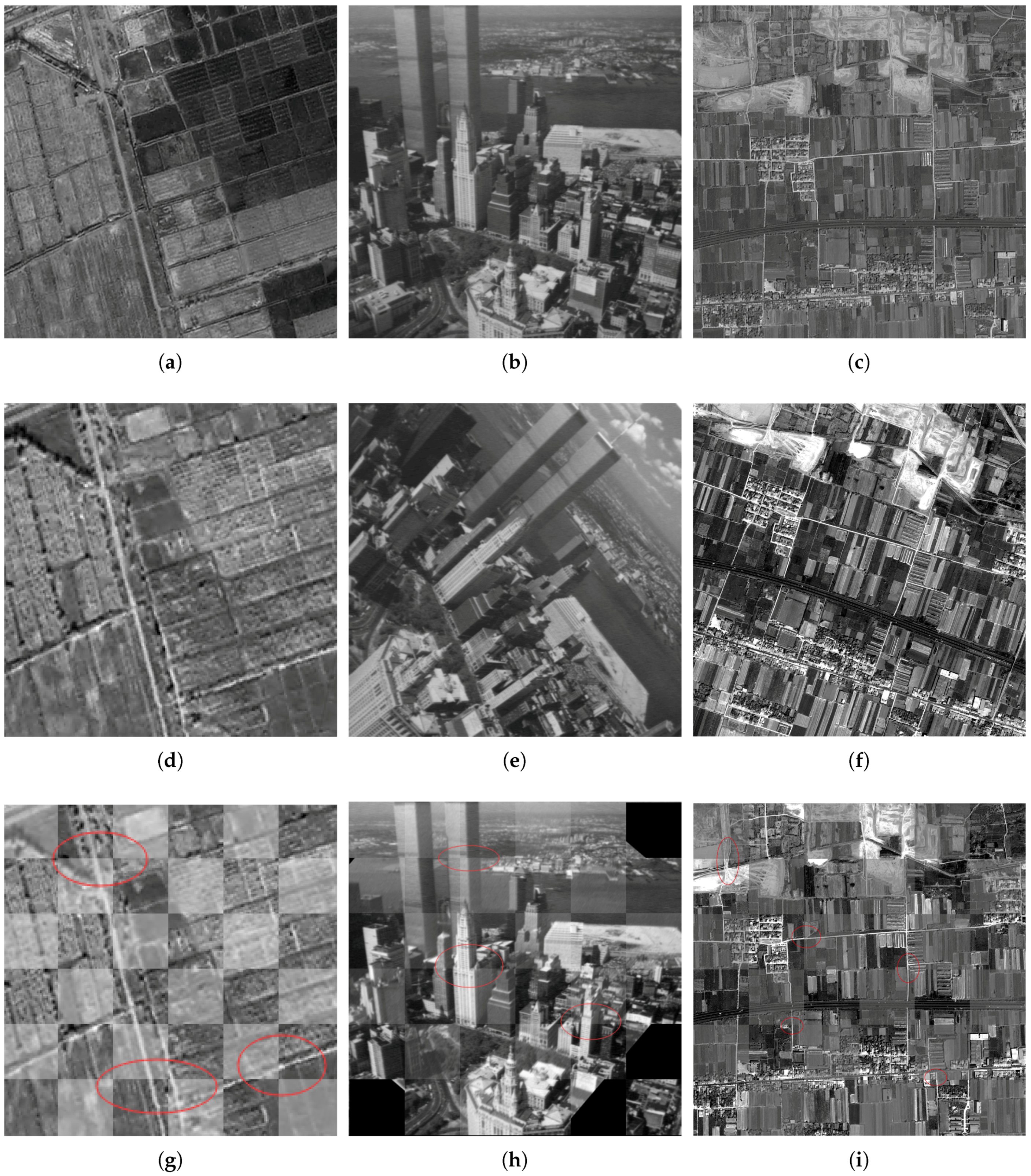
4.1. Qualitative Experiment

In this section, three pairs of images are registered by the proposed algorithm, MPFT, and then a checkerboard visualization of registered images is shown to illustrate the effectiveness of the proposed algorithm. The three pairs of images, shown in Figure 6, illustrate the scale difference, angle rotation, and similarity transform, respectively. Due to the large spatial extent of all images, certain regions are denoted with red ellipses to indicate the effectiveness of the MPFT. Through the careful inspection, the result matching is satisfied, even for the images with a significant gray difference and a slight change in content, which illustrates the practical value of the proposed MPFT algorithm.

4.2. Quantitative Experiment

This section describes three experiments—an interpolation error comparison experiment and synthetic and real data experiments—that were carried out to verify the performance of the proposed method, MPFT. At the same time, two other competitive phase correlation based registration algorithms, the Pseudo-polar Fourier transform method (PPFT) [39] and the Multilayer Fractional Fourier Transform method (MLFFT) [41] were used for comparison. Although these two methods were proposed years ago, they are also the state-of-the-art algorithms due to the absence of the development of novel and effective phase correlation methods in recent years. To compare the performance of the proposed method more thoroughly, we also compared it to the most classical feature-based image registration method, SIFT [11] and its variant, mode-seeking SIFT (ms-SIFT) [19], which is used for similarity estimations. The SIFT algorithm was implemented by VLFeat [47] and ms-SIFT was implemented by us in accordance with the original related paper [19]. In each experiment, there were two kinds of parameters to be set for the phase correlation-based algorithm. One type was related to the construction of the log-polar grid (polar grid) and included the number of radial lines, the number of points in a single radial line, and the log-base ${\rho }_0$. The other type concerned the algorithm itself. Fo MLFFT and MPFT, there was one parameter to be specified: the number of single grids. For PPFT, there were no parameters to be set. The concrete parameter settings for each experiment are detailed in

Table 1. The details of parameters to be set in each experiment.

Experiment		Constuction of the Log-Polar Grid (or Polar Grid)			Number of Single Grids
		Size $\mathit{M}\times \mathit{N}$		Log-Base $\left({\mathit{\rho }}_0\right)$	MPFT	MLFFT
		Number of Radial Lines $\left(\mathit{M}\right)$	Number of Points in the Radial Line $\left(\mathit{N}\right)$
Numerical Experiment		…	…	1.044	4	4
Synthetic Data Experiment	Similarity Transform Estimation Angle Estimation	128	128	${\left(\frac{\pi }{0.015}\right)}^{\frac{1}{127}}$	4	4
		250	250	–	1	4
Real Data Experiment		128	128	${\left(\frac{\pi }{0.015}\right)}^{\frac{1}{127}}$	4	4
Further Analysis		128	128	…	4	4

Note: ’–’ represents there is no need to set this parameter (there is no parameter ${\rho }_0$ for the polar grid); ’…’ represents a series value. (The concrete value series are described in the corresponding section).

.

During the process of determining the scaling factors for each single polar grid, the the log-polar radius series values were partioned by the MATLAB function histcounts. The experiments were carried out on a desktop computer with Intel Xeon CPU 3.50GHz, 16-GB memory, and MATLAB R2017B. In the synthetic and real data experiments, two measurements were used to evaluate the performance of each algorithm. One was the mean absolute estimation error, which represents the accuracy of each algorithm in estimating the scale and angles. It was computed by using the formula $\frac{1}{C}{\sum }_n|s_n^{\prime }-s_n|$, where $s_n^{\prime }$ denotes the estimation value, $s_n$ is the truth value for the image pair n, and C is the total number of image pairs. The other was the root-mean-square error (RMSE), which denotes the robustness of the performance algorithm. It can be calculated by the expression $\sqrt{\frac{1}{C}{\sum }_n{(s_n^{\prime }-s_n)}^2}$.

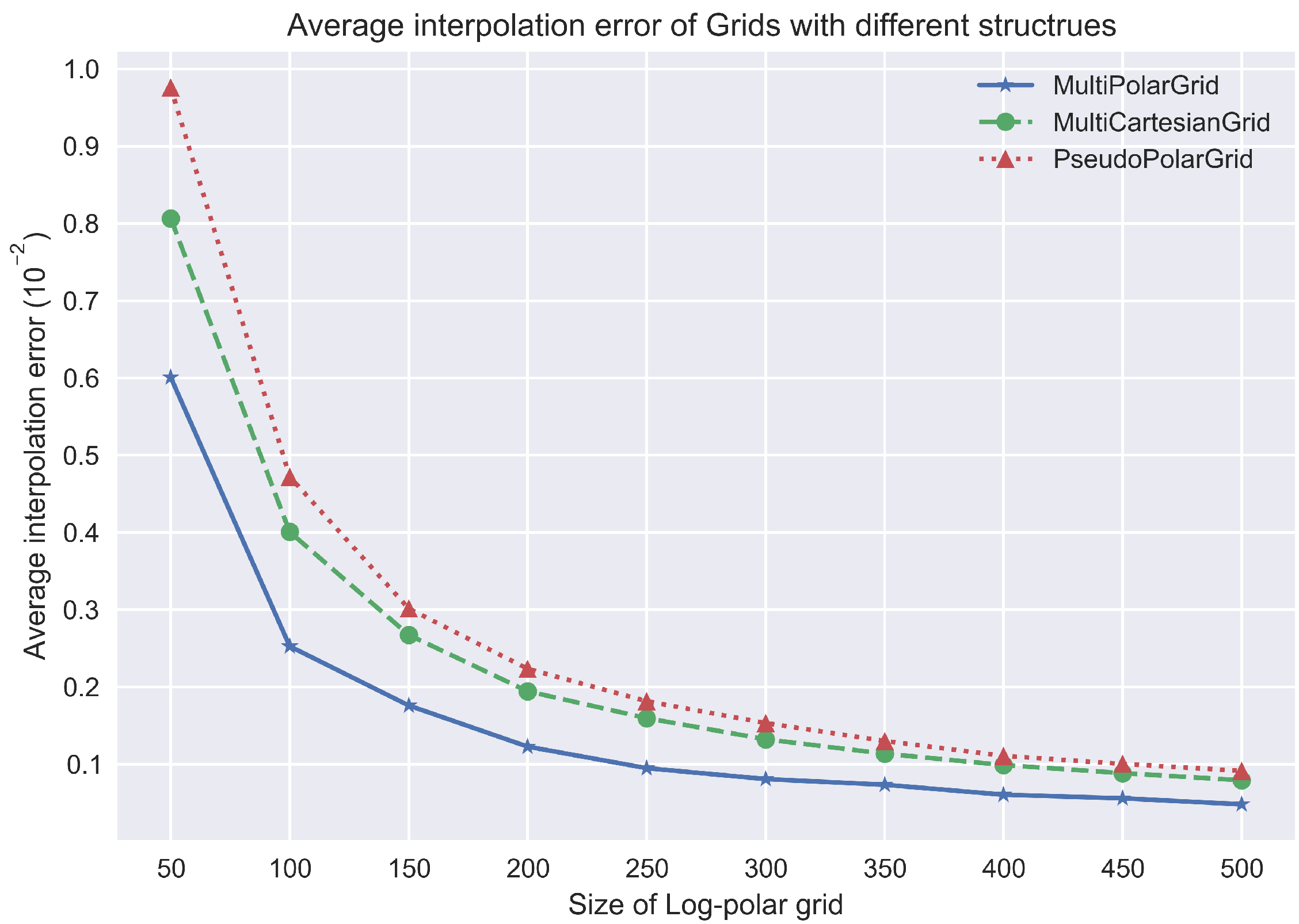
4.2.1. Numerical Simulation of the Interpolation Error

The most basic requirement for the estimation of scales and angles based on phase correlation is the accurate calculation of the log-polar Fourier transform. Under the framework of interpolating the log-polar Fourier transform, the interpolation error can be measured by the mean squared Euclidean distance between the actual point in the log-polar frequency plane and the closest point in the interpolated grids. The three different algorithms have different grid structures: the MultiPolarGrid (MPFT method), the MultiCartesianGrid (MLFFT method), and the PseudoPolarGrid (PPFT method). These grids were utilized to compare the interpolation errors. For these experiments, the number of layers was set to four in the MultiPolarGrid and the MultiCartesianGrid, which was consistent with the subsequent synthetic and real data experiments. So, four polar grids constituted the final MultiPolarGrid and MultiCartesianGrid. The scaling factor of each polar grid was acquired by partitioning the log-polar radius series values into four bins. For the log-polar grid, the log-base ${\rho }_0$ was set to $1.044$. The average interpolation error was equal to the accumulated Euclidean distance divided by the total number of destination grid points. The size of the log-polar varied from $50\times 50$ to $500\times 500$ in steps of 50. A comparison of the average interpolation error of the grids with three different structures is shown in Figure 7. Obviously, the MultiPolarGrid has a smaller interpolation error than the other two grids; the MultiCartesianGrid has the second lowest interpolation error. In addition, the advantage of MultiPolarGrid is particularly evident, especially for small-sized images, which is greatly helpful to attaining success and higher accuracy in patch-based matching.

4.2.2. Synthetic Data Experiments

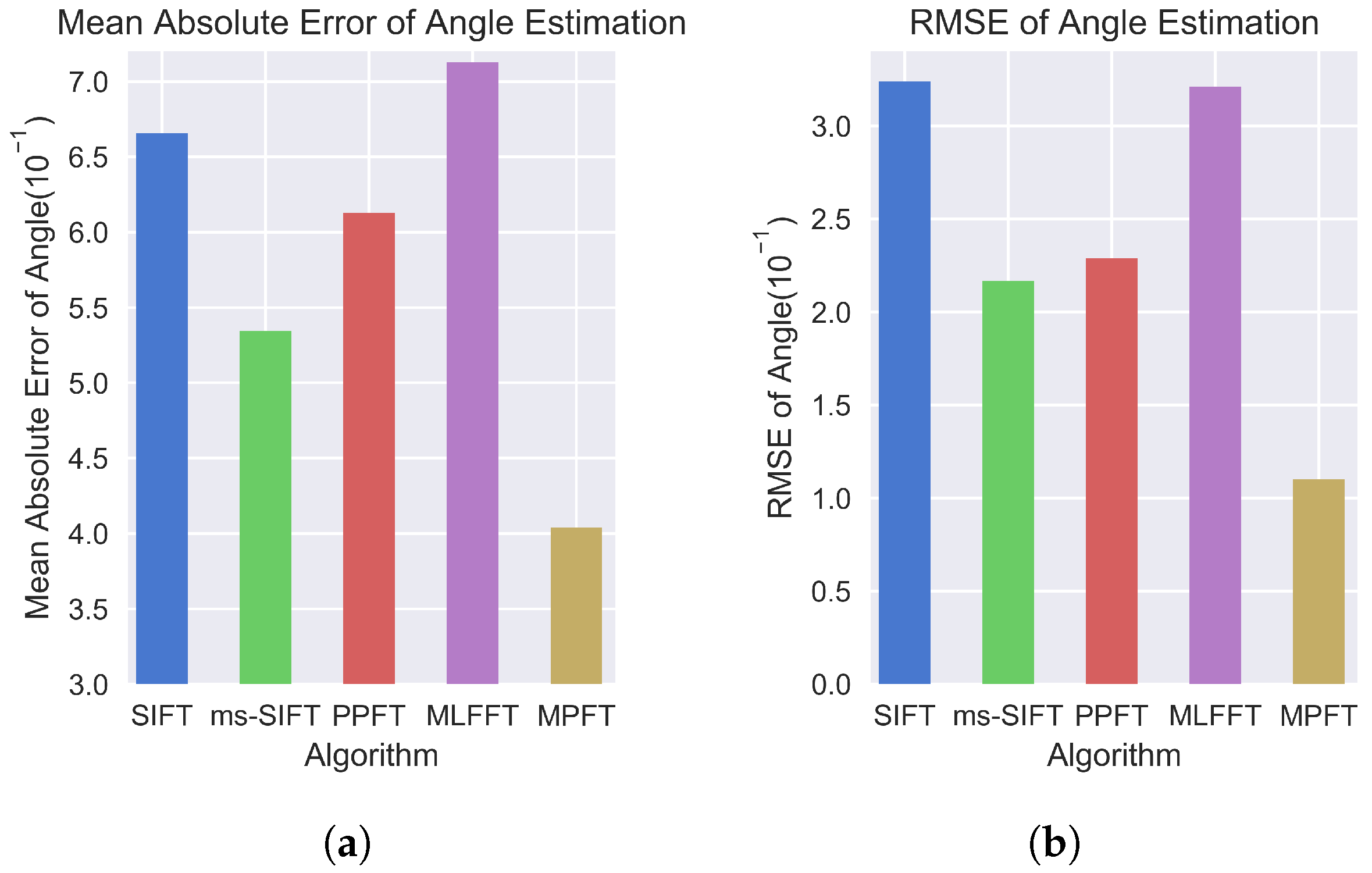
Two sets of simulation experiments were carried out. One was the case of only angle transformation. Because the specificity of the polar Fourier transform is only sufficient for angle estimation and MPFT can calculate the Fourier transform accurately, this was used to demonstrate the effect of the accurate Fourier transform. The other was the case of similarity transformation. The main goal of this was to assess the performance of the proposed method when the shift, rotation, and scale exist simultaneously.

Angle Estimation

For angle estimation only, there is no need to construct the log-polar grid—the polar grid is enough. For MPFT, the destination grid is the polar grid. So, the number of layers of MPFT was set to 1. Images with a size of $1024\times 1024$ pixels from different sensors, as in the following similarity transformation, were utilized. There were 80 images in total. Each image was rotated by a random angle. The range of rotation angles was from 0° to 180°. After rotating the image, a pair of images with a size of $512\times 512$ pixels, centered at the rotated image and original image, respectively, were clipped as the final estimated image pairs. Due to the large rotations, the final estimated image pairs had different contents, which made the angle estimation more challenging. The mean absolute error and RMSE of each algorithm are shown in Figure 8.

From Figure 8, it is evident that the feature-based methods SIFT and ms-SIFT perform better than MLFFT, but worse than the proposed algorithm, MPFT. The proposed algorithm, MPFT, has the best performance among all of the competitive algorithms, and the MLFFT has the worst performance. The PPFT algorithm is superior to the SIFT method, but inferior to ms-SIFT. Among the phase correlation-based algorithms, the great success of MPFT is mainly due to its lack of interpolation error when calculating the polar grid Fourier transform, while the other two algorithms have interpolation errors when calculating the polar grid Fourier transform. Interestingly, the MLFFT had a worse performance than the PPFT here although the number of layers of the MultiCartesianGrid was four. An in-depth analysis identified two reasons for this. One is that the PseudoPolarGrid of PPFT is more similar to the polar grid compared to the MultiCartesianGrid of MLFFT. The other reason is that the points in a radial line of the polar grid are evenly spaced while most of the points in a radial line of the log-polar grid are cluttered within a smaller radius. The difference means that using the MultiCartesianGrid to approximate a polar grid will lead to a larger error, so MLFFT has the worst performance for the angle rotation only case. This implies that the accuracy of the polar Fourier transform has a large influence on angle estimation.

Similarity Transformation Estimation

In this experiment, images from different sensors—GF-1, GF-2, Sentinel-2 and ZY-03—were used to carry out the simulated data experiment. The content of images varied: farmlands, roads, buildings, mountains and so on. One example image for each sensor is shown in Figure 9. Their sizes were all $800\times 800$ pixels. There were a total of 80 images, with an equal amount from each of the aforementioned four sensors. Each image was shifted, rotated, and scaled randomly to make the registration problem more challenging. The range of shift was 0 to half of the image size; scaling values varied from $0.1$ to 10; and the rotation angle was within the range of 0°to 90°. For each image pair, we used the SIFT, ms-SIFT, MPFT, MLFFT, and PPFT algorithms to estimate the scale and rotation parameters. To quantify the performance of each algorithm, two measurements for scale and angle were used: the average absolute error and the root-mean-square error. The bar diagram for the performance of each algorithm is shown in Figure 10.

Obviously from Figure 10, we can see that the SIFT algorithm has almost the worst performance for both the scale and angle estimation, except that its mean absolute error of scale is lower than that of PPFT. ms-SIFT performs better than PPFT except its RMSE of angle estimation is higher than that of PPFT, but worse than MLFFT and MPFT. In the comparison between only phase-based methods, PPFT has the worst performance and MLFFT has the second worst performance. This is because although the PPFT grid separates the plane into BH and BV parts (BH and BV are two subsets of points defined in [39]), its radial lines are evenly sloped and deviate from the radial lines with equal angle intervals in the structure of the log-polar grid. For MLFFT, although there are four combined Cartesian grids with different scaling factors, its single Cartesian grid is very different from the structure of the log-polar grid. The robustness of MLFFT is strong; it can always acquire a middle ranking result. MPFT has the best performance among all other methods in both scale and angle estiamtion. This is because the polar-grid has the same angularly equispaced radial lines as the ones of log-polar grids. The only difference from the log-polar grid is that the points in the radial line are evenly spaced, while the points in the radial lines of the log-polar grid are exponentially spaced. However, the gap between these points in the radial line can be narrowed by the combination of multiple polar grids with different scaling factors.

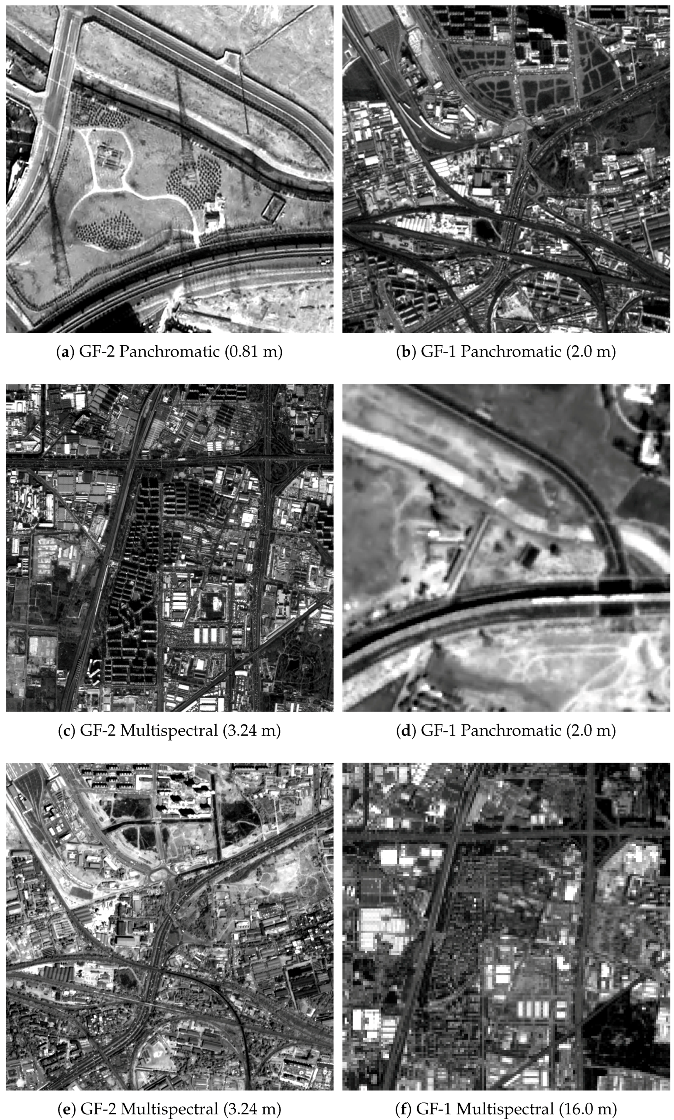
4.2.3. Real Experiments and Analysis

This subsection describes the performance of two sets of experiments. One applied the registration algorithm directly to estimate the similarity transform between images of a small size. The other registered the scenes of remote sensing by adoption of the tiling strategy. The registration algorithm was only utilized to estimate the similarity transform between corresponding tiles to acquire tie points. Then, these tie points were used to fit a transform model of scenes to rectify the scenes.

4.2.3.1. Estimation of the Similarity Transform between Remote Sensing Images Directly

Three groups of remote sensing images with 45 pairs of images in total from GF-1 and GF-2 were utilized. Their descriptive information is listed in

Table 2. The metadata of remote sensing images with similarity transformation

Category	Sensed Image	Reference Image	Number of Image Pairs
I	Sensor: GF-2 Panchromatic Resolution: 0.81 m Size: 512 × 512 Acquisition Data: November 2017	Sensor: GF-1 Panchromatic Resolution: 2.0 m Size: 207 × 207 Acquisition Data: June 2013	15
II	Sensor: GF-1 Panchromatic Resolution: 2.0 m Size: 829 × 829 Acquisition Data: June 2013	Sensor: GF-2 Multispectral Resolution: 3.24 m Size: 512 × 512 Acquisition Data: November 2017	15
III	Sensor: GF-2 Multispectral Resolution: 3.24 m Size: 800 × 800 Acquisition Data: June 2013	Sensor: GF-1 Multispectral Resolution: 16 m Size: 162 × 162 Acquisition Data: November 2017	15

. Three examples from different group data sets are shown in Figure 11. All the image pairs with a similarity transform relationship were acquired by the process of pre-orthorectification. For high-resolution satellite images captured by narrow field-of-view cameras, the absolute positioning errors arising from the initial RPC model are likely to be near constant throughout the scene and amenable to compensation via a small translation and rotation of the image coordinates [48]. Consequently, after pre-orthorectification using the initial RPC model and auxiliary digital elevation model (DEM) data, most of the complex deformations of the raw image can be corrected (approximately remaining a translation, scale difference and small rotation), and therefore, the processed images have only a similarity deformation. The SIFT, ms-SIFT, MPFT, MLFFT and PPFT algorithms were applied to estimate the similarity transform. Due to the unknown rotation angle and translation parameter for each image pair, we used the errors of corresponding points from the registered and reference images to evaluate the performances of the different algorithms. The corresponding points were selected by using the open-source toolbox VLFeat [47]. Then, the errors of each corresponding point were evaluated using three measurements, $e_x$, $e_y$ and $e={(e_x^2+e_y^2)}^{1/2}$, where $e_x$ and $e_y$ represent the root-mean-square errors (RMSE) in the x and y directions, respectively. The overall registration error of an image pair was estimated as the average error of a certain number of matched points. According to the principle of keypoint location in the process of point detection, the keypoints detected in the first octave with the original image size have higher location accuracy than keypoints detected in other octaves. After rectifying the images, the registered images had almost the same scale. So, only keypoints with higher location accuracy in the first octave were kept for the specific evaluation of each algorithm. Then, ten corresponding points evenly distributed in the image were selected for each image pair. The measurements $e_x$, $e_y$ and e for each method represent the corresponding average measurements of all image pairs, respectively. The maximum absolute error of $MA{X}_x$ in the x direction and $MA{X}_y$ in the y direction were also measured. The results are summarized in

Table 3. Three average measurements $e_x$, $e_y$ and e for each algorithm (pixel).

Algorithm	${\mathit{e}}_{\mathit{x}}$	${\mathit{MAX}}_{\mathit{x}}$	${\mathit{e}}_{\mathit{y}}$	${\mathit{MAX}}_{\mathit{y}}$	e
SIFT	0.8041	1.6291	0.7203	1.8937	1.1908
ms-SIFT	0.6291	1.5721	0.6715	1.6382	0.9925
PPFT	0.7052	1.4650	0.7133	1.5320	1.1201
MLFFT	0.6183	1.3952	0.6201	1.3905	0.9729
MPFT	0.5623	1.3815	0.5738	1.3902	0.9017

$e_x$ and $e_y$ denote the root-mean-square errors (RMSE) in the x and y directions, respectively. $e={(e_x^2+e_y^2)}^{\frac{1}{2}}$ $MA{X}_x$ and $MA{X}_y$ denote the maximum absolute errors in the x and y directions, respectively. The bold numbers indicate the minimum value in each column.

.

From Table 3, we can easily find that the MPFT method has the best performance for all measurements compared with the other four algorithms and SIFT has the worst performance. This result is also consistent with the synthetic data experiments. For the SIFT algorithm, the non-linear gray difference and changes in content between image pairs result in many mismatching points, which reduces the registration accuracy. Compared to SIFT, the ms-SIFT algorithm improves the overall match obtained by performing mode seeking to eliminate the outlying corresponding points. However, its accuracy is also lower than that of MLFFT and MPFT. Among the phase correlation based algorithms, the main advantage of MPFT is that it can reduce the error produced when calculating the log-polar transform to the minimum compared to the other two algorithms, which significantly improves the registration accuracy.

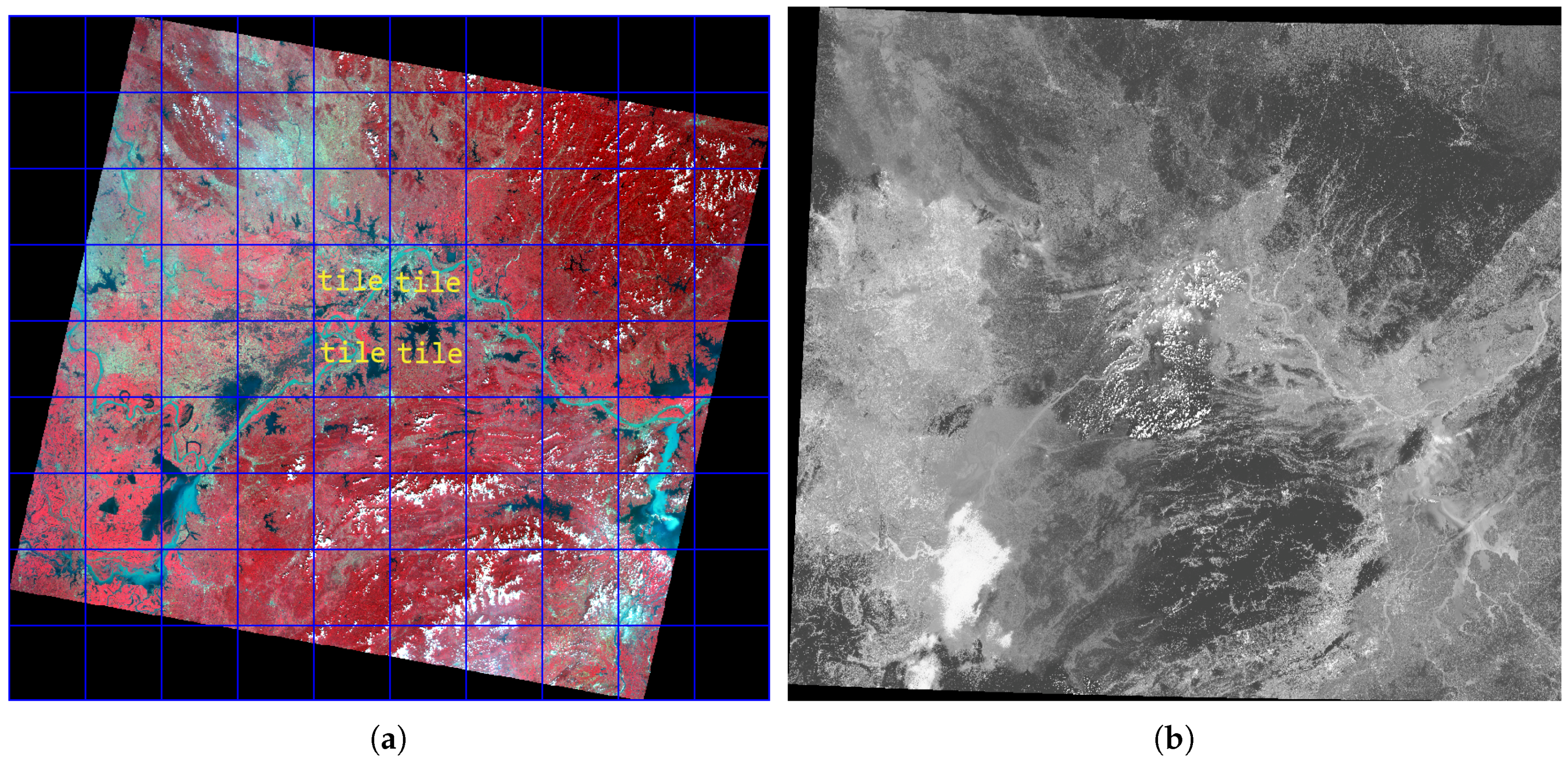
4.2.3.2. Register Scenes of Remote Sensing by Tiling

The data used for the experiment were one scene of a Landsat 8 panchromatic image with a resolution of 15 m and one scene of a HJ-1 level 2 image with a resolution of 30 m. The main applications of the HJ-1 satellite, launched by the National Disaster Reduction Center of China (NDRCC) in 2008 are environmental monitoring and prediction, solid waste monitoring, and disaster monitoring and prediction. They are shown in Figure 12. The premise of registration is that, after initial geometric model correction, the deformation of the local region is displacement dominated, along with small scale and rotation differences. The specific registration strategy used involved resampling the Landsat 8 image to 30 m, dividing the HJ-1 image into many tiles ($256\times 256$ pixes), and then roughly locating corresponding tiles of the same size according to the projected coordinate information. The centroids of each pair of tiles were regarded as the initial tie points. We applied the PPFT, MLFT, and MPFT methods to estimate the similarity transform of each corresponding pair, and utilized the acquired similarity transform to correct each pair of initial tie points to obtain the final control points. In addition, a phase correlation-based method (called the PC method) was also applied to estimate the displacement of each tile pair instead of the similarity transform. Lastly, a terrain-dependent RPC model [49] fitted to all the final control points, combined with the random sampling consensus algorithm (RANSAC), was utilized to correct the whole image. After rectification, fifty checkpoints, distributed evenly in the image, were selected manually to validate the final registration accuracy in terms of three measurements, $e_x$, $e_y$ and e, the same as in the experiment where the similarity transform was estimated directly Section 4.2.3.1. $MA{X}_x$ and $MA{X}_y$ denote the maximum absolute errors in the x and y directions, respectively. The experimental report is given in

Table 4. Three average measurements $e_x$, $e_y$ and e, for each algorithm (pixel).

Algorithm	${\mathit{e}}_{\mathit{x}}$	${\mathit{MAX}}_{\mathit{x}}$	${\mathit{e}}_{\mathit{y}}$	${\mathit{MAX}}_{\mathit{y}}$	e
PC	1.3671	3.1459	0.5196	1.5505	1.4625
PPFT	1.2539	2.3720	0.4912	1.2318	1.3466
MLFFT	1.1997	2.2225	0.5187	1.8221	1.3071
MPFT	1.0850	2.1370	0.4385	1.4062	1.1703

$e_x$ and $e_y$ denote the root-mean-square errors (RMSE) in the x and y directions, respectively. $e={(e_x^2+e_y^2)}^{\frac{1}{2}}$. $MA{X}_x$ and $MA{X}_y$ denote the maximum absolute errors in the x and y directions, respectively. The bold numbers indicate the minimum value in each column.

.

The experimental results in Table 4 show that the PC method, which only estimates the displacement of local tiles, has the worst performance compared to the other three methods that estimate the displacement, small rotation, and scale. It is illustrated that the estimation of the slight rotation and scale of local tiles can improve the final registration accuracy, especially in the case of high estimation accuracy of scale and angle. In terms of e, MLFFT is slightly better than MPFT, but for $e_y$, the opposite is true. MPFT is better than all of the other methods in terms of $e_x$, $e_y$, and e. Although the $MA{X}_y$ of MPFT is not the minimum and it ranks second, we can also conclude that it performs best considering the minor difference between its value of $MA{X}_y$ and the minimum of $MA{X}_y$.

5. Discussion

5.1. Analysis of the Parameter Settings

To construct a log-polar grid, three parameters are required: the number of radial lines M, the number of points in each radial line N, and the log-base ${\rho }_0$. In fact, it was found through experiments that the parameters M and N do not produce intrinsic effects on the accuracy of the estimation of angle and scale differences when they are greater than 128. In most cases, both M and N were set to 128, which was enough to guarantee high accuracy. However, the log-base ${\rho }_0$ affects the success or failure of the estimation of large scale differences in practical applications. It is crucial to use a proper value for the parameter log-base ${\rho }_0$. Thus, another 16 image pairs consisting of GF-2 panchromatic images with a resolution of 0.81 m and ZY-02C multispectral images with a resolution of 10 m were used to test the effect of the value of log-base ${\rho }_0$. Their scale difference reached 12. Here, the determination of ${\rho }_0$ was used to determine the minimum radius $r_0$ in the log-polar grid. When the number of points in a radial line is fixed, the log-base ${\rho }_0$ can be calculated according to the minimum radius value $r_0$, namely ${\rho }_0={\left(\frac{\pi }{r_0}\right)}^{\frac{1}{N}}$ . Note that due to the properties of the logarithm operation, the minimum radius $r_0$ is not set to zero. In this study, for synthetic and real images, the $r_0$ was set to $0.015$ and $0.021$, respectively. However, for the image pairs with a scale difference of 12, when the $r_0$ is greater than $0.001$, the phase correlation-based image registration does not estimate the scale difference successfully. The phase correlation-based scale estimation only works when the $r_0$ is less than $0.001$. At this time, it is noteworthy that the smaller $r_0$ becomes, the larger ${\rho }_0$ becomes, the lower the estimation accuracy of the scale is, and the points in a radial line are clustered within a smaller radius. As for how well $r_0$ is set, this is also an open problem. However, a rough conclusion is drawn that the larger the scale difference is, the greater ${\rho }_0$ should gradually become .

5.2. Analysis of Performance

In the experiment Section 4, firstly, a qualitative experiment, the registration of three pairs of images with scale, rotation, and similarity transform was carried out. The checkerboard view shows that the alignment is well done, which illustrates the effectiveness of the proposed algorithm, MPFT.

Accurate calculation of the log-polar Fourier transform is critical for the estimation of the similarity transform based on phase correlation. Compared to PPFT and MLFFT, MPFT can acquire the most accurate log-polar Fourier transform. The average interpolation distance error experiment was theoretically illustrated by a numerical experiment. MPFT was shown to always have the minimum interpolation error for different log-polar grid sizes, with PPFT having the maximum interpolation error.

To estimate the similarity transform for remote sensing images, both synthetic and real data experiments were carried out. Compared to the competitive algorithms SIFT, ms-SIFT, PPFT, and MLFFT, the performance of MPFT ranked first. Large non-linear gray differences, slight content changes, and areas without salient features, result in many mismatching points or less matching points of high quality when SIFT is used directly, which heavily lowers the performance of SIFT. ms-SIFT improves the performance of SIFT by filtering out a large number of initial matches and retaining a set of reliable correspondences with the help of mode-seeking. ms-sIFT also performs better than PPFT, but is inferior to MPFT and MLFFT. For the three phase correlation-based algorithms, PPFT, MLFFT and MPFT, MPFT has the best performance, and MLFFT performs better than PPFT. However, in the case of angle estimation only, the polar Fourier transform is enough. MLFFT has the worst performance compared to the other algorithms due to its poor ability to approximate the polar Fourier transform, and MPFT performs better than the other algorithms due to its lack of interpolation error in the calculation of the polar Fourier transform. The performance ranking difference of MLFFT and MPFT in the similarity transform estimation and only angle estimation experiment further illustrates that the calculation of the log-polar Fourier transform (or polar Fourier transform) greatly affects the registration accuracy based on phase correlation, and MPFT can acquire the best accuracy of estimation for the similarity transform.

At last, a pair of scenes in HJ-1 and Landsat 8 images were registered based on phase correlation. Four algorithms, PC, PPFT, MLFFT and MPFT, were compared. The PC algorithm is a category in itself because it only estimates the displacement of corresponding tiles and other three algorithms estimate the similarity transform of corresponding tiles. In fact, the PC algorithm performed worse than other three algorithms, which illustrates the importance of estimating the similarity transform in remote sensing registration. In the comparison of the three algorithms that estimate the similarity transform (PPFT, MLFFT, and MPFT), MPFT showed the highest accuracy in terms of the $e_x$, $e_y$ and e values of manually selected checkpoints. This also supports the idea that MPFT has a higher accuracy of estimation of the similarity transform than the MLFFT and PPFT algorithms.

5.3. Analysis of Efficiency

As for the efficiency of MPFT, due to the different implementation languages, the use of C++ for the core source code of the feature-based algorithm and MATLAB code for the phase correlation-based algorithms, and because the processing time of the feature-based algorithm varies with the image content while that of the phase correlation-based algorithm is only dependent on the size of image, we only compared the processing times of the three phase correlation-based algorithms: PPFT, MLFFT, and MPFT. An in-depth analysis of the procedures of the three algorithms showed that their only difference is in the calculation of the log-polar Fourier transform. So, only the computation time of the log-polar Fourier transform for the three algorithms was compared. Two thousand pairs of synthetic images, with different scaling, rotation and shift were utilized to compare the processing times. These images had the same size of $256\times 256$ pixels. Each algorithm was run 2000 * 5 times and the corresponding parameters were the same, as in the real experiment. The average processing times of PPFT, MLFFT, and MPFT were 2.35 seconds, 3.48 seconds, and 6.17 seconds, respectively. Although PPFT is faster than MLFFT and MPFT, its performance is the worst. Compared to MLFFT, MPFT has a longer computation time due to the use of more “for loops” in its implementation. Considering its distinguished performance, the efficiency difference is relatively small, and the gap can be further narrowed by the usage of compiled programming language, such as C++ programming language. Besides, due to the characteristics of the MPFT algorithm (as expressed in Formula 21), it is easy to parallelize. In particular, with the explosive improvement in computing capability of CPU and GPU today, its processing time can be further reduced and the efficiency can be further improved.

5.4. Analysis of Applicability and Limitations

The proposed algorithm, MPFT, which can estimate the similarity transform accurately, is essentially a phase correlation-based displacement registration method. It utilizes the property that the scale and angles of the Cartesian coordinates can be converted into the displacement of the log-polar coordinates. When the geometric deformations between images are complex, a linear relationship between the phase difference in the frequency domain and the displacement in the spatial domain will become weak or will even no longer be valid. So, for MPFT, as long as the deformation between images can be approximated by the similarity transform after coarse rectification, it can be used to register them.

In our experiments, after pre-orthorectification using the RPC model and auxiliary DEM data, the deformations of the corresponding small tiles tiled from the remote sensing scenes were displacement dominant, along with small rotation and scale differences. So, the deformation between these small tiles can be reasonably regarded as the similarity transform. The proposed method can accurately estimate the similarity transform between tiles. After the correction of each pair of tiles, their central points can be treated as a pair of control points. With the use of these generated control points and a proper transform model, remote sensing scenes can be registered.

For other categories of images, the same is true. For example, for images with relief displacement, the relief displacement can be corrected by the usage of a DEM and imaging model, and the deformation of images can be reasonably approximated as a similarity transform. So, the MPFT can register them. However, if the effect of the relief displacement is not reduced or eliminated due to the lack of availability of an accurate DEM or imaging model, the geometric deformation between them cannot be regarded as a similarity transform. In this case, the MPFT will fail to match them. For aerial images or oblique images, the initial geometric deformation is more complex than a similarity transform; if there is a possibility that after coarse rectification of images, the left deformation between them can be regarded as a similarity transform, the MPFT can be used to register them.

6. Conclusions

In this paper, a novel phase correlation-based algorithm, the Multilayer Polar Fourier Transform (MPFT) was proposed, which is able to estimate the rotation and scale parameters between images more accurately than the other two phase correlation-based algorithms, the Multilayer Fractional Fourier Transform (MLFFT) and the Pseudo-polar Fourier Transform (PPFT), and the classical feature-based algorithm, SIFT, and its variant, ms-SIFT. The image pairs for estimation can be multi-source remote sensing images acquired at different times. It is possible for some images to suffer from non-linear photometric change, occlusion by cloud, or a small amount of content change. MPFT inherits the high accuracy of phase correlation-based image registration and extends itself to estimate the scale and angle parameters accurately, which expands the scope of the application of the phase correlation method. In the future, we will focus on the sensitivity of log-polar Fourier transform-based image registration.

References

1. Brown, L.G. A survey of image registration techniques. ACM Comput. Surv. (CSUR) 1992, 24, 325–376. [Google Scholar] [CrossRef] [Green Version]
2. Zitova, B.; Flusser, J. Image registration methods: A survey. Image Vis. Comput. 2003, 21, 977–1000. [Google Scholar] [CrossRef]
3. Behling, R.; Roessner, S.; Segl, K.; Kleinschmit, B.; Kaufmann, H. Robust automated image co-registration of optical multi-sensor time series data: Database generation for multi-temporal landslide detection. Remote Sens. 2014, 6, 2572–2600. [Google Scholar] [CrossRef]
4. Modersitzki, J. Numerical Methods for Image Registration; Oxford University Press: Oxford, UK, 2004. [Google Scholar]
5. Sundaresan, A.; Varshney, P.K.; Arora, M.K. Robustness of change detection algorithms in the presence of registration errors. Photogramm. Eng. Remote Sens. 2007, 73, 375–383. [Google Scholar] [CrossRef]
6. Yan, L.; Roy, D.P.; Zhang, H.; Li, J.; Huang, H. An automated approach for sub-pixel registration of Landsat-8 Operational Land Imager (OLI) and Sentinel-2 Multi Spectral Instrument (MSI) imagery. Remote Sens. 2016, 8, 520. [Google Scholar] [CrossRef]
7. Dai, X.; Khorram, S. The effects of image misregistration on the accuracy of remotely sensed change detection. IEEE Trans. Geosci. Remote Sens. 1998, 36, 1566–1577. [Google Scholar]
8. Liu, Y.; Mo, F.; Tao, P. Matching Multi-Source Optical Satellite Imagery Exploiting a Multi-Stage Approach. Remote Sens. 2017, 9, 1249. [Google Scholar] [CrossRef]
9. Stumpf, A.; Michéa, D.; Malet, J.P. Improved Co-Registration of Sentinel-2 and Landsat-8 Imagery for Earth Surface Motion Measurements. Remote Sens. 2018, 10, 160. [Google Scholar] [CrossRef]
10. Long, T.; Jiao, W.; He, G.; Zhang, Z. A fast and reliable matching method for automated georeferencing of remotely-sensed imagery. Remote Sens. 2016, 8, 56. [Google Scholar] [CrossRef]
11. Lowe, D.G. Distinctive image features from scale-invariant keypoints. Int. J. Comput. Vis. 2004, 60, 91–110. [Google Scholar] [CrossRef]
12. Wang, S.; Quan, D.; Liang, X.; Ning, M.; Guo, Y.; Jiao, L. A deep learning framework for remote sensing image registration. ISPRS J. Photogramm. Remote Sens. 2018, 145, 148–164. [Google Scholar] [CrossRef]
13. Tong, X.; Li, L.; Liu, S.; Xu, Y.; Ye, Z.; Jin, Y.; Wang, F.; Xie, H. Detection and estimation of ZY-3 three-line array image distortions caused by attitude oscillation. ISPRS J. Photogramm. Remote Sens. 2015, 101, 291–309. [Google Scholar] [CrossRef]
14. Almonacid-Caballer, J.; Pardo-Pascual, J.E.; Ruiz, L.A. Evaluating fourier cross-correlation sub-pixel registration in landsat images. Remote Sens. 2017, 9, 1051. [Google Scholar] [CrossRef]
15. Skakun, S.; Roger, J.C.; Vermote, E.F.; Masek, J.G.; Justice, C.O. Automatic sub-pixel co-registration of Landsat-8 Operational Land Imager and Sentinel-2A Multi-Spectral Instrument images using phase correlation and machine learning based mapping. Int. J. Dig. Earth 2017, 10, 1253–1269. [Google Scholar] [CrossRef]
16. Scheffler, D.; Hollstein, A.; Diedrich, H.; Segl, K.; Hostert, P. AROSICS: An automated and robust open-source image co-registration software for multi-sensor satellite data. Remote Sens. 2017, 9, 676. [Google Scholar] [CrossRef]
17. Reddy, B.S.; Chatterji, B.N. An FFT-based technique for translation, rotation, and scale-invariant image registration. IEEE Trans. Image Process. 1996, 5, 1266–1271. [Google Scholar] [CrossRef] [PubMed]
18. Stone, H.S.; Tao, B.; McGuire, M. Analysis of image registration noise due to rotationally dependent aliasing. J. Vis. Commun. Image Represent. 2003, 14, 114–135. [Google Scholar] [CrossRef]
19. Kupfer, B.; Netanyahu, N.S.; Shimshoni, I. An Efficient SIFT-Based Mode-Seeking Algorithm for Sub-Pixel Registration of Remotely Sensed Images. IEEE Geosci. Remote Sens. Lett. 2015, 12, 379–383. [Google Scholar] [CrossRef]
20. Sedaghat, A.; Ebadi, H. Accurate affine invariant image matching using oriented least square. Photogramm. Eng. Remote Sens. 2015, 81, 733–743. [Google Scholar] [CrossRef]
21. Sedaghat, A.; Ebadi, H. Remote sensing image matching based on adaptive binning SIFT descriptor. IEEE Trans. Geosci. Remote Sens. 2015, 53, 5283–5293. [Google Scholar] [CrossRef]
22. Ye, Y.; Shan, J.; Bruzzone, L.; Shen, L. Robust registration of multimodal remote sensing images based on structural similarity. IEEE Trans. Geosci. Remote Sens. 2017, 55, 2941–2958. [Google Scholar] [CrossRef]
23. Sedaghat, A.; Mokhtarzade, M.; Ebadi, H. Uniform robust scale-invariant feature matching for optical remote sensing images. IEEE Trans. Geosci. Remote Sens. 2011, 49, 4516–4527. [Google Scholar] [CrossRef]
24. Sedaghat, A.; Mohammadi, N. Uniform competency-based local feature extraction for remote sensing images. ISPRS J. Photogramm. Remote Sens. 2018, 135, 142–157. [Google Scholar] [CrossRef]
25. Ye, Y.; Shan, J.; Hao, S.; Bruzzone, L.; Qin, Y. A local phase based invariant feature for remote sensing image matching. ISPRS J. Photogramm. Remote Sens. 2018, 142, 205–221. [Google Scholar] [CrossRef]
26. Li, J.; Hu, Q.; Ai, M.; Zhong, R. Robust feature matching via support-line voting and affine-invariant ratios. ISPRS J. Photogramm. Remote Sens. 2017, 132, 61–76. [Google Scholar] [CrossRef]
27. Argyriou, V.; Vlachos, T. A Study of Sub-Pixel Motion Estimation Using Phase Correlation; BMVC: York, UK, 2006; pp. 387–396. [Google Scholar]
28. Tian, Q.; Huhns, M.N. Algorithms for subpixel registration. Comput. Vis. Graph. Image Process. 1986, 35, 220–233. [Google Scholar] [CrossRef]
29. Abdou, I.E. Practical approach to the registration of multiple frames of video images. In Proceedings of the International Society for Optics and Photonics, Visual Communications and Image Processing ’99, San Jose, CA, USA, 28 December 1998; Volume 3653, pp. 371–383. [Google Scholar]
30. Stone, H.S.; Orchard, M.T.; Chang, E.C.; Martucci, S.A. A fast direct Fourier-based algorithm for subpixel registration of images. IEEE Trans. Geosci. Remote Sens. 2001, 39, 2235–2243. [Google Scholar] [CrossRef] [Green Version]
31. Liu, J.G.; Yan, H. Robust phase correlation methods for sub-pixel feature matching. In Proceedings of the 1st Annual Conference System Eng. Autonomous System Defence Technology Centre, Edinburgh, UK, 7–9 September 2006; p. A13. [Google Scholar]
32. Liu, J.; Yan, H. Phase correlation pixel-to-pixel image co-registration based on optical flow and median shift propagation. Int. J. Remote Sens. 2008, 29, 5943–5956. [Google Scholar] [CrossRef]
33. Tong, X.; Xu, Y.; Ye, Z.; Liu, S.; Li, L.; Xie, H.; Wang, F.; Gao, S.; Stilla, U. An improved phase correlation method based on 2-D plane fitting and the maximum kernel density estimator. IEEE Geosci. Remote Sens. Lett. 2015, 12, 1953–1957. [Google Scholar] [CrossRef]
34. Hoge, W.S. A subspace identification extension to the phase correlation method [MRI application]. IEEE Trans. Med. Imaging 2003, 22, 277–280. [Google Scholar] [CrossRef] [PubMed] [Green Version]
35. Tong, X.; Ye, Z.; Xu, Y.; Liu, S.; Li, L.; Xie, H.; Li, T. A novel subpixel phase correlation method using singular value decomposition and unified random sample consensus. IEEE Trans. Geosci. Remote Sens. 2015, 53, 4143–4156. [Google Scholar] [CrossRef]
36. Leprince, S.; Barbot, S.; Ayoub, F.; Avouac, J. Automatic, precise, ortho-rectification and co-registration for satellite image correlation, application to seismotectonics. IEEE Trans. Geosci. Remote Sens 2007, 45, 1529–1558. [Google Scholar] [CrossRef]
37. Dong, Y.; Long, T.; Jiao, W.; He, G.; Zhang, Z. A novel image registration method based on phase correlation using low-rank matrix factorization with mixture of Gaussian. IEEE Trans. Geosci. Remote Sens. 2018, 56, 446–460. [Google Scholar] [CrossRef]
38. Chen, Q.; Defrise, M.; Deconinck, F. Symmetric phase-only matched filtering of Fourier-Mellin transforms for image registration and recognition. IEEE Trans. Pattern Anal. Mach. Intell. 1994, 16, 1156–1168. [Google Scholar] [CrossRef]
39. Keller, Y.; Averbuch, A.; Israeli, M. Pseudopolar-based estimation of large translations, rotations, and scalings in images. IEEE Trans. Image Process. 2005, 14, 12–22. [Google Scholar] [CrossRef] [PubMed] [Green Version]
40. Liu, H.; Guo, B.; Feng, Z. Pseudo-log-polar Fourier transform for image registration. IEEE Signal Process. Lett. 2006, 13, 17–20. [Google Scholar]
41. Pan, W.; Qin, K.; Chen, Y. An adaptable-multilayer fractional Fourier transform approach for image registration. IEEE Trans. Pattern Anal. Mach. Intell. 2009, 31, 400–414. [Google Scholar] [CrossRef] [PubMed]
42. Moisan, L. Periodic plus smooth image decomposition. J. Math. Imaging Vis. 2011, 39, 161–179. [Google Scholar] [CrossRef] [Green Version]
43. Dong, Y.; Long, T.; Jiao, W. Eliminating effect of image border with image decomposition for phase correlation based image registration. In Proceedings of the 2018 IEEE International, Geoscience and Remote Sensing Symposium (IGARSS), Valencia, Spain, 23–27 July 2018. [Google Scholar]
44. Abbas, S.A.; Sun, Q.; Foroosh, H. An Exact and Fast Computation of Discrete Fourier Transform for Polar and Spherical Grid. IEEE Trans. Signal Process. 2017, 65, 2033–2048. [Google Scholar] [CrossRef]
45. Bailey, D.H.; Swarztrauber, P.N. The fractional Fourier transform and applications. SIAM Rev. 1991, 33, 389–404. [Google Scholar] [CrossRef]
46. Averbuch, A.; Coifman, R.R.; Donoho, D.L.; Elad, M.; Israeli, M. Fast and accurate polar Fourier transform. Appl. Comput. Harmon. Anal. 2006, 21, 145–167. [Google Scholar] [CrossRef]
47. Vedaldi, A.; Fulkerson, B. VLFeat: An open and portable library of computer vision algorithms. In Proceedings of the 18th ACM international conference on Multimedia, Firenze, Italy, 25–29 October 2010; pp. 1469–1472. [Google Scholar]
48. Fraser, C.S.; Dial, G.; Grodecki, J. Sensor orientation via RPCs. ISPRS J. Photogramm. Remote Sens. 2006, 60, 182–194. [Google Scholar] [CrossRef]
49. Long, T.; Jiao, W.; He, G. RPC Estimation via 1-Norm-Regularized Least Squares (L1LS). IEEE Trans. Geosci. Remote Sens. 2015, 53, 4554–4567. [Google Scholar] [CrossRef]
Figure 1. Overall workflow of the proposed method
Remotesensing 10 01719 g001
Figure 2. The relationship between the error of the estimated scale and the log-base ρ 0 . For each fixed scale, the estimated scale error increases almost linearly with the log-base ρ 0 .
Remotesensing 10 01719 g002
Figure 3. Schematic of the polar grid. The size of the points has no extra meaning; the smaller sized points are only used for clear visualization.
Remotesensing 10 01719 g003
Figure 4. In Figure (a), after uniformly scaling the Cartesian grid on the x axis (scaling the x coordinates of all of the points by a proper factor cos Δ θ and keeping their y coordinates unchanged), all the red circle points in the two green radical dashed lines fall exactly on the vertical lines that constitute the Cartesian grid scaled on the x axis. In Figure (b), after uniformly scaling the Cartesian grid on the y axis (scaling the y coordinates of all of the points by a proper factor cos ( 90° Δ θ ) and keeping their x coordinates unchanged), all the red circle points in two green dashed lines fall exactly on the horizontal lines that constitute the Cartesian grid scaled on the y axis.
Remotesensing 10 01719 g004
Figure 5. (ad) have scaling factors of 0.25, 0.51, 0.76, and 1.0 respectively. (e) is the overlay of the former four single polar grids with different scaling factors. (f) is the destination log-polar grid. Each grid has 16 radial lines that are angularly equispaced and 24 points on each radial line.
Remotesensing 10 01719 g005
Figure 6. (a,d) are a pair of images with a scale difference of 2.5. They are from the panchromatic bands of GF-1 and GF-2, respectively; (g) is the checkerboard visualization of the registered images; (b,e) are a pair of images with a rotation angle difference of about 50°; (h) is the checkerboard visualization of matched images; (c,f), from the panchromatic bands of GF-1 and GF-2, respectively, are a pair of images, with both a scale difference of about 2.5, a rotation difference of about 20°, and displacement differences of about 49 pixels and 74 pixels in the x and y directions, respectively; (i) is the checkerboard visualization of rectified images.
Remotesensing 10 01719 g006
Figure 7. Average interpolation error of grids with different structures. The size of the log-polar grid varies from 50 × 50 to 500 × 500 .
Remotesensing 10 01719 g007
Figure 8. (a) is the mean absolute error of the angle estimation, (b) is the RMSE of the angle estimation.
Remotesensing 10 01719 g008
Figure 9. Example images of similarity transformation. (a) is the GF-1 panchromatic image, covering the farmland and buildings; (b) is the Sentiment-2A images, mainly containing mountains and roads; (c) is the GF-2 panchromatic image, consisting of man-made buildings; (d) is a ZY-03 image, including the plain area.
Remotesensing 10 01719 g009
Figure 10. Comparison of performance of the SIFT, ms-SIFT, PPFT, MLFFT, and MPFT algorithms in estimating scale and angle. (a) is the mean absolute error of scale estimation, (b) is the RMSE of the scale estimation, (c) is the mean absolute error of angle estimation, and (d) is the RMSE of angle estimation.
Remotesensing 10 01719 g010
Figure 11. Three examples of remote sensing image pairs from GF-1 and GF-2 with similarity transform. Each column is a pair of images (namely, (a,d), (b,e), (c,f) are image pairs, respectively).
Remotesensing 10 01719 g011
Figure 12. (a) is one scene of HJ-1, whose resolution is 30 m, (b) is one scene of the Landsat 8 panchromatic image with a resolution of 15 m. The images cover the area of Wuhan in China. The main contents of the image are rivers, mountains and residential areas. The differences between images are that some areas are covered by cloud, and some ground features are different. The reference image a is divided into many tiles, as shown in the blue grid, and each small blue grid denotes a tile.
Remotesensing 10 01719 g012