Article

Extracting Individual Bricks from a Laser Scan Point Cloud of an Unorganized Pile of Bricks

1
School of Earth Sciences and Engineering, Hohai University, No. 8, Fochengxi Road, Nanjing 211100, China
2
Department of Geoscience and Remote Sensing, Delft University of Technology, Stevinweg 1, 2628 CN Delft, The Netherlands
*
Authors to whom correspondence should be addressed.
Remote Sens. 2018, 10(11), 1709; https://doi.org/10.3390/rs10111709
Submission received: 21 August 2018 / Revised: 19 October 2018 / Accepted: 26 October 2018 / Published: 29 October 2018

Abstract

:
Bricks are the vital component of most masonry structures. Their maintenance is critical to the protection of masonry buildings. Terrestrial Light Detection and Ranging (TLidar) systems provide massive point cloud data in an accurate and fast way. TLidar enables us to sample and store the state of a brick surface in a practical way. This article aims to extract individual bricks from an unorganized pile of bricks sampled by a dense point cloud. The method automatically segments and models the individual bricks. The methodology is divided into five main steps: Filter needless points, brick boundary points removal, coarse segmentation using 3D component analysis, planar segmentation and grouping, and brick reconstruction. A novel voting scheme is used to segment the planar patches in an effective way. Brick reconstruction is based on the geometry of single brick and its corresponding nominal size (length, width and height). The number of bricks reconstructed is around 75%. An accuracy assessment is performed by comparing 3D coordinates of the reconstructed vertices to the manually picked vertices. The standard deviations of differences along x, y and z axes are 4.55 mm, 4.53 mm and 4.60 mm, respectively. The comparison results indicate that the accuracy of reconstruction based on the introduced methodology is high and reliable. The work presented in this paper provides a theoretical basis and reference for large scene applications in brick-like structures. Meanwhile, the high-accuracy brick reconstruction lays the foundation for further brick displacement estimation.

Graphical Abstract

1. Introduction

Terrestrial Light Detection and Ranging (TLidar) provides 3D coordinates of a scene by measuring distances between the scanner’s center and the points on the object surface in a spherical coordinate system. The distances are commonly computed by measuring the time delay or phase shift between the emission and return of a laser beam. In addition, the horizontal and the vertical angle of the laser beams transmitted with predefined horizontal and vertical increments are recorded. The TLidar system is regarded as the center (origin) in such coordinate system. Due to its ability to provide dense and accurate measurements, TLidar has been already successfully applied in various fields related to civil engineering, such as road modeling [1,2], deformation analysis [3,4,5], change detection [6,7,8], cultural heritage [9,10,11] and health monitoring [12,13]. Specific applications for masonry structures containing tiny bricks/stones can be seen in ref. [14], which reported on a point cloud acquired by TLidar used to automatically reconstruct the armor cubes from rubble mound breakwaters. Besides this, a new methodology was presented for the 3D outline extraction of concrete armor units in a breakwater, which enabled the estimation of displacements and rotation of these units [15]. More recently, a 3-D morphological method was proposed to change analysis of a beach with seagrass berm using TLS, in which a cost-efficient, accurate and quick tool was used to reconstruct the sand volume in natural and artificial replenished beaches [16].
Point clouds gathered through TLidar consist of massive amounts of unorganized data that should be processed accordingly, which has already become a vital bottleneck for the implementation of the TLidar technology. As a basic step for surface reconstruction, point cloud segmentation plays a key role in the further analysis. Segmentation is the process that collects similar surface points into single feature surfaces. The accuracy of this process will inevitably influence the result of consecutive processing. Point clouds are usually unorganized, noisy, sparse, lack semantic information [17], have inconsistent point density, various surface shape, and their handling is therefore rather difficult and complex.
Diverse methods and algorithms for segmentation have been suggested and proposed in literature. In ref. [18], they are categorized into three types: (1) edge-based methods [19,20], where edge points are first identified, then geometrical attributes, e.g., normal, curvature, gradient, in a cross-section perpendicular to the edge dividing different surfaces, were computed to segment the surface. Edge-based methods are sensitive to noise because of the sensitivity of geometrical attributes (e.g., curvature) to noise, while smoothing will influence the estimation results as well. (2) Region-based methods [21,22] are where local neighborhood properties are used to search for similarity within a specific feature or to find variation among features. Then the surface is segmented by merging spatially close points. Compared to edge-based methods, region-based methods are more robust to noise. However, region-based methods may lead to over or under segmentation. Also, the difficulty of localizing region edges accurately needs to be resolved. (3) hybrid methods [23,24], as the name suggests, combine edge-based and region-based information to overcome deficiencies and limitations involved in aforementioned approaches.
Actually, most scenarios have surface shapes that can be represented by primitive surfaces such as planes, cylinders, cones and spheres. In this respect, an object model is always regarded as the composition of such primitives. Various methods and algorithms for different intrinsic surfaces were proposed and improved. Genetic algorithms (GA) were used to extract quadric surfaces [25]. Furthermore, GA was combined with an improved robust estimator to extract planar and quadric surfaces [26]. A framework for the segmentation of multiple objects from a 3D point cloud was presented in [27], which provided quantitative and visual results based on the so-called attention-based method. Random Sample Consensus (RANSAC) was implemented to segment planar regions from 3D scan data [28]. A 3D Hough Transform was used to segment continuous planes in point-cloud data, the results of which were compared to RANSAC [29]. The 3D Hough Transform was also implemented for sphere recognition and segmentation [30]. A fast approach for surface reconstruction by means of approximate polygonal meshing was proposed, and a state-of-the-art performance was achieved which was significantly faster than other methods [31].
Many studies have already reported on the problems in the segmentation of 3D point clouds. One problem is that it is hardly possible to determine the structure or the mathematical model of a surface sampled by a raw point cloud. Certainly, a series of solutions have been proposed. However, while resolving the problem, new issues may emerge, e.g., ambiguity induced by the overlap of different objects, algorithms are sensitive to noise, et al. In this regard, the segmentation problem still requires more attention, especially for some specific applications such as segmenting point clouds sampling ancient, irregular buildings, disordered stones, and so on. In our research, we focus on planar segmentation since the objects (regular bricks) are composed of planar patches. Additionally, most man-made structures in reality also consist of planar surface, therefore, this focus gives the research a wider applicability.
A step possibly following segmentation is 3D reconstruction. For points sampling the 3D object surface, the objective of the reconstruction problem is to recover the geometric shape from the point cloud. To solve this problem, diverse algorithms have been proposed and implemented, which fall into three categories: (1) sculpting-based method, in which the surface is reconstructed using methods from computational geometry, e.g., using a Delaunay triangulation [32], Boissonnat method [33], alpha-shape [34], graph-based [35] and crust algorithm [36]. (2) contour-tracing methods, in which the surface is approximated [37]. (3) region growing methods, in which a seed triangle patch is determined, and new triangles are added to the mesh under construction [38]. In our research, considering that the research object is a brick with a regular shape, a simplified model is sufficient to present the semantic information of the brick, which focuses on estimating patches and brick vertices, assuming each brick can be approximated by a cuboid.
This article aims at developing and testing a reliable methodology to segment and reconstruct the bricks in a pile of bricks. For this purpose, terrestrial Lidar data were used as a basic source to identify the geometry of each individual brick. To optimize the use of this technique and avoid manual processing, an approach that automates the segmentation of single brick unit is developed. Meanwhile, a data-driven method for extracting the vertices of the bricks and reconstructing the bricks is proposed. Comparing this process with the existing approaches, our method is able to semantically recognize the bricks and provide geometric information. The reason to work with a pile of bricks is twofold. First, such piles are easily available for experiments as reported on in this manuscript, while the problem is actually not so easy to solve. Second, the method developed to solve the problem can be applied in different scenarios. Directly, for every similar problems, e.g., ref. [15], or, after some adaption, for other problems considering bricks, stones or boulders. Possible applications could include rock glaciers [39], rockfall [40], and assessing the state of archeological masonry structures [41]. Foreseen scenario’s include change detection. Therefore, the focus here to detect brick visible by the scanner. In future work the methodology used in this manuscript could be used to compare visible brick positions before and after an event, like a rock fall, or a partial collapse of a city wall. The article starts with an introduction; then, Section 2 introduces the study area and data acquisition; afterwards, 
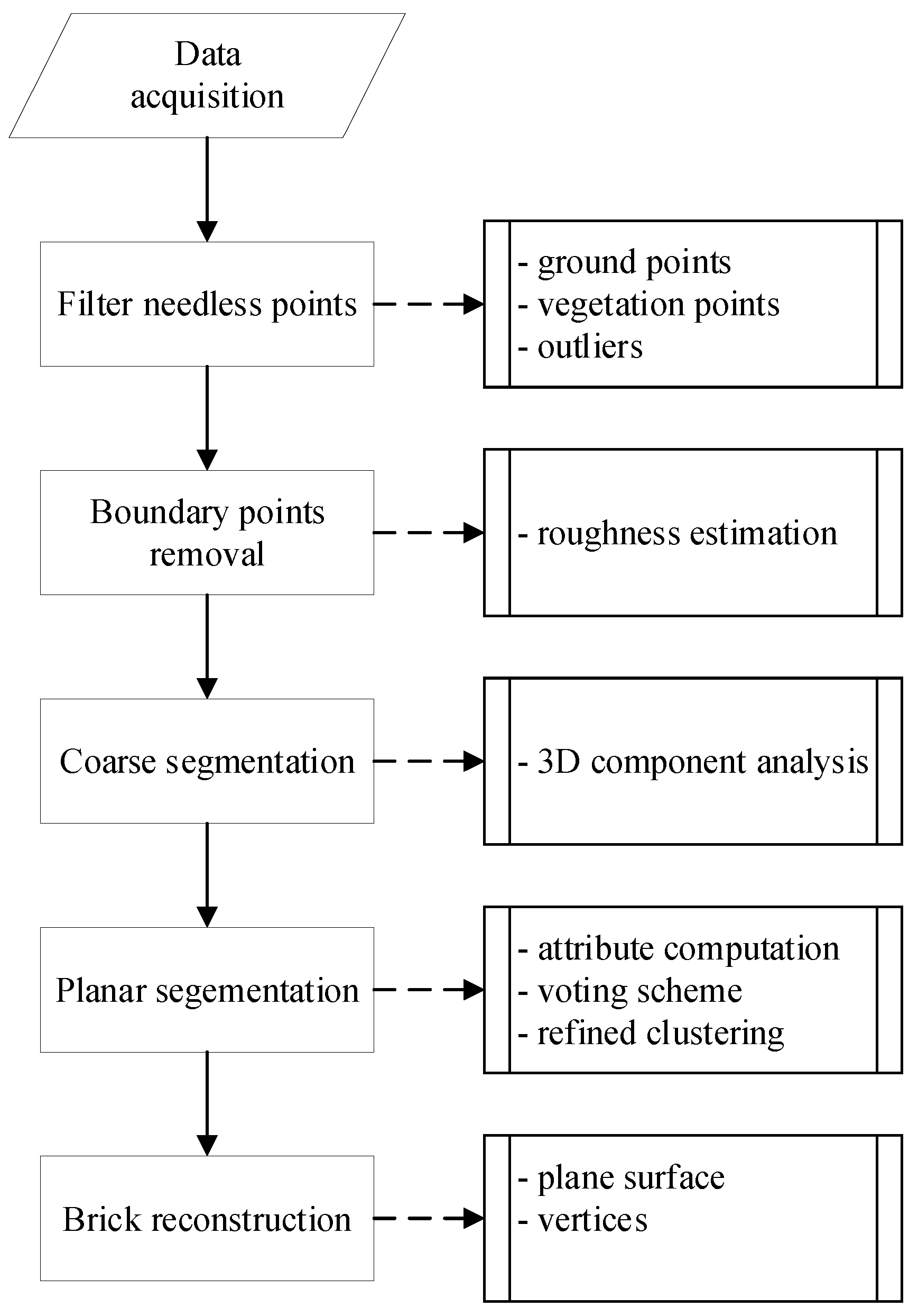
Section 3 presents the developed methodology, which consists of five steps: (1) filter needless (i.e., outliers, ground points, vegetation points, etc.) points, (2) brick boundary points removal, (3) coarse segmentation using 3D component analysis, (4) planar segmentation and grouping, (5) brick reconstruction. Section 4 presents the segmentation and reconstruction results, and the accuracy assessment of the reconstruction is shown as well. Section 5 presents discussion of the proposed methodology, applications and future works. Finally, the conclusions are discussed in Section 6.

2. Materials

2.1. Experimental Area

In order to test the developed methodology, an experiment composing of the sampling scattered bricks was designed and carried out. Figure 1 is a picture of the piles of bricks taken from the perspective of the scanner station.

2.2. Scan Data Acquisition

In the experiment, scan data acquisition was performed using the FARO LS-880 Laser Scanner (FARO, Lake Mary, FL, USA) which is a phase-shift scanner operating with a range of 360° in horizontal and 320° in vertical. The angular resolutions of the scanner are 0.009° and 0.00076° in horizontal and vertical, respectively. The nominal linear accuracy of this scanner is ±3 mm (one sigma) at ranges up to 25 m in normal illumination and reflectivity conditions. One station is planned at a distance of approximately 6 m from the center of the pile to acquire the 3D point cloud of the piles of bricks. To improve visibility, the terrestrial Lidar was set at ~1.5 m height. The raw point cloud acquired by the FARO Laser Scanner included about 1.5 million points. Figure 2 shows the raw point cloud colored.

3. Methods

Data acquired using the TLidar resulted in a 3D point cloud. The proposed geometry extraction and modelling procedures include five main steps: (1) filter needless points; (2) remove the boundary points of the bricks; (3) coarse segmentation using 3D component analysis; (4) planar segmentation; (5) brick reconstruction. The workflow is summarized in Figure 3.

3.1. Filter Needless Points

Once the 3D point cloud for the research scene is acquired, it is essential to filter outliers and the needless points backscattered by ground, vegetations, et al. The filtering process is divided into three steps. First, thanks to the scanner being levelled during the scanning, the ground points could be filtered coarsely based on height information. Points on the ground have minimum Z coordinate [42]. Thus, a threshold is defined to detect and remove ground points, the value of which is determined by the accuracy of the scanning, i.e., two times of the nominal accuracy of the scanner with the value of 6 mm. Next, point normal vectors are estimated. Through incorporating the point normal which is estimated by PCA and the Z coordinate, points on the ground are determined and removed coarsely. This implementation of the process is first to search the points with the Z value less than 6 mm in the local area. The next step is to search the nearest neighbor points for a given point with a pre-defined number of 50. Based on the neighbor points, the PCA is used to estimate the normal vector for the given point, i.e., the third component of the PCA results denotes the normal vector. The normal vectors of the ground points are expected to be parallel to the Z axis. Thus, an angular difference threshold of one degree is used to determine the ground points, i.e., if the angular difference between the normal vector and the Z axis is less than one degree, the given point is regarded as the ground point. Afterwards, a method is adopted to remove vegetation points, in which vegetation and non-vegetation are classified through a curvature index [43]. In other words, points in vegetation show a high curvature index, since foliage points do not show a clear structure. An eigen values analysis of the local covariance matrix is used to estimate the curvature for each point, as described below:
Let ( x i , y i , z i ) , i = 1 , 2 , , n be n points of the scene. For the current 3D point p i = ( x i , y i , z i ) in the point cloud, the information of its local neighborhood is determined using k nearest neighbors (in our study, k value is set as 300). Thus, the covariance matrix for the neighborhoods is defined as:
3 × 3 = 1 k i = 1 k ( p i p ) ( p i p ) T  
where p = 1 k i = 1 k ( x i , y i , z i ) is the mean of the nearest neighbours of k . The covariance matrix in Equation (1) describes the geometric characteristics of the underlying local surface. The Singular Value Decomposition (SVD) is used to decompose into eigenvectors which are sorted in descending order according to the composing eigenvalues λ i ( i = 2 , 1 , 0 ,       0 λ 0 λ 1 λ 2 ) [44]. The eigenvalues λ 2 , λ 1 and λ 0 correspond to the eigenvectors v 2 , v 1 and v 0 , respectively. v 0 approximates the surface normal of the current point p i and the elements of the eigenvector v 0 are used to fix the parameters of a plane through the neighborhood of p i . The smallest eigenvalue λ 0 describes the variation along the surface normal and indicates if points are spatially consistent [45]. In most cases, the curvature is used to describe the surface variation along the direction of the corresponding eigenvalues, the value of which is estimated as
σ ( p i ) = λ 0 λ 0 + λ 1 + λ 2  
The value σ ( p i ) also reflects whether the current point p i and its neighbors are coplanar [46]. In this way, the distribution of curvatures for all points are obtained and vegetation points are recognized and removed. As demonstrated in ref. [46], it is commonly accepted that if a λ 0 value of greater than 20%, these points would be regarded as vegetation points. Finally, outliers as well as remaining ground points and vegetation points are detected and removed based on local point density. Compared to the brick points, outliers, remaining ground points and vegetation points always have relative lower local density.

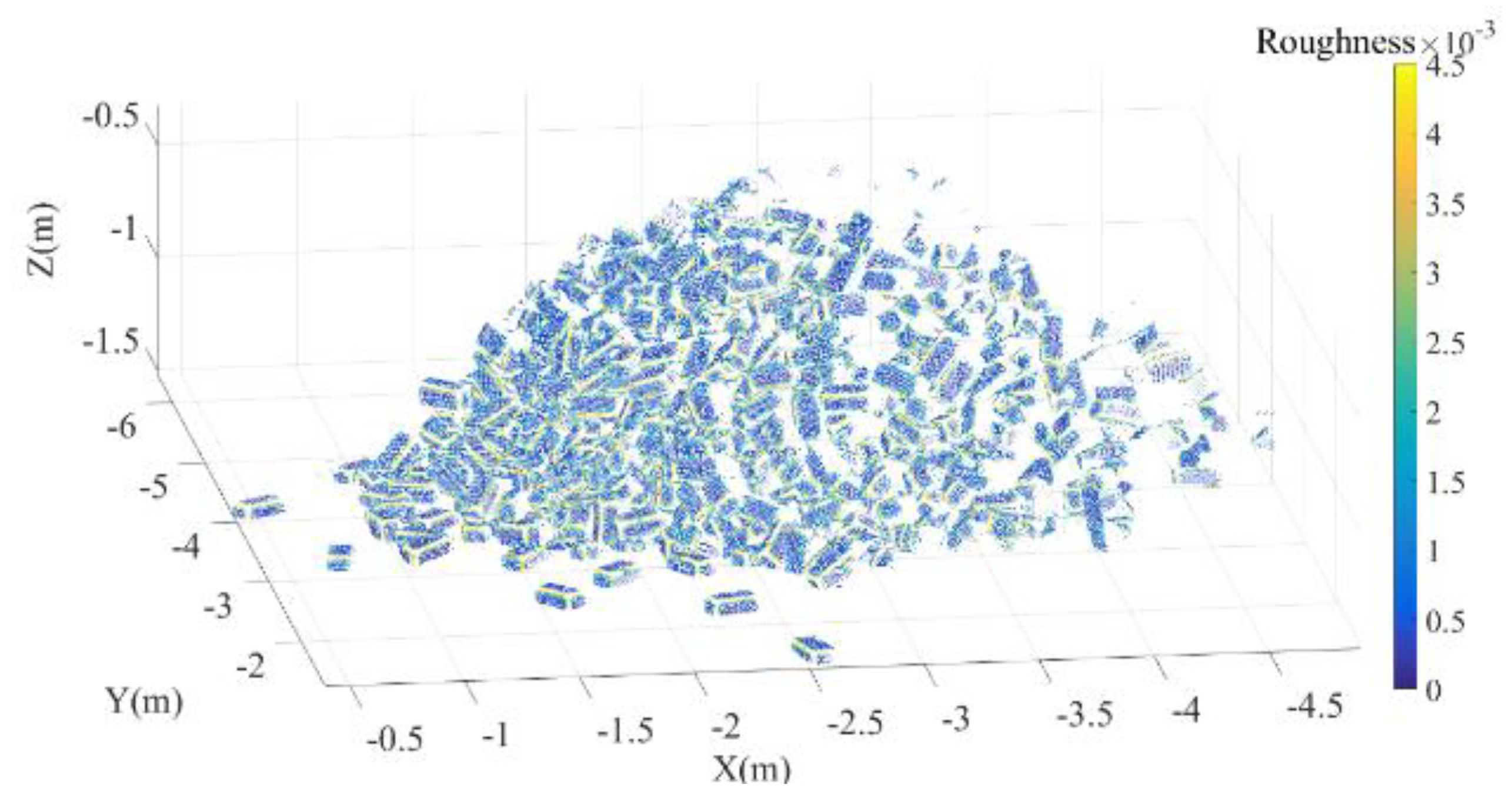
3.2. Roughness Estimation

For each point, its roughness value is defined as the distance between this point and the best fitting plane estimated from its nearest neighbors. The plane is fitted by least squares to the K nearest neighbors (KNN) [47,48] of a target point. The procedure is done as follows:
(1) Search the K-nearest neighbors of the target point and extract their coordinates. K is the input parameter to the algorithm defined by the user (in our study, K is set as 50).
(2) A Least squares algorithm [49] is implemented based on the searched points and the plane equation is estimated.
(3) Calculate the distance between the target point to the fitted plane which is regarded as roughness value.
(4) Traverse every point in the point cloud and execute step (1) to step (3). In this way, the roughness values for all points are determined.
Afterwards, point classification is done based on the roughness. It is evident that the variance of roughness is relatively small in the middle of a brick surface and large on the edges, at the corners of the bricks and at outliers. Points with smaller variance are adopted as seeds in the further analysis.
Here, it should be noted that if the points on edges, the corners of the bricks and the outliers are not discarded, the following segmentation is probably incomplete. Since the bricks are piled in an irregular way, typically only points from each individual brick are spatially connected. Therefore, it is hard separating individual bricks in a regular way.

3.3. Coarse Segmentation Using 3D Connected Component Analysis

Once the roughness computation and the brick edge points removal have been done, it is possible to initiate the brick surface segmentation. A 3D connected component algorithm [50,51,52] is used to realize the coarse segmentation. The accuracy of connected component labelling is the base of the latter parts.
The points on the object are represented by 3D coordinates, the connected component analysis is therefore extended to 3D. A 3D connected component counting and labelling algorithm in [53,54] was applicable to small neighborhoods and effective for many classification tasks. It is specified for local neighborhoods, and 3D grid (voxel) deduced from octree structure is used to extracted the connected components. Here, neighborhoods voxels with a size of 3 × 3 × 3 are used. The central voxel in a 3 × 3 × 3 neighborhood has three types of neighbors: (1) 6-connectivity, 6 voxels are sharing a face with the central voxel. (2) 18-connectivity, in addition 12 voxels are sharing an edge with the central voxel. (3) 26-connectivity, in addition 8 voxels are sharing a point with the central voxel.
In our work, face connected neighbors are used to segment the bricks as implemented in the Cloudcompare software (Paris, France) [55]. Ideally, points from different bricks are classified into different components after the implementation of the 3D connected component analysis. However, owing to the complicated position relation between the adjacent bricks, some bricks may still belong to the same component although the edge points have already been removed.

3.4. Planar Segmentation and Grouping

Once the coarse segmentation is completed, the next step is the surface plane detection for individual bricks. The workflow for plane detection is summarized in Figure 4.

3.4.1. Attribute Computation Using Neighboring Points

The geometric features for a given point are derived from the spatial arrangement of all 3D points within a neighborhood. For this purpose, some attributes such as distances, angles, and angular variations have been proposed in refs. [56,57]. In our research, point attributes were computed based on the neighboring points identified by a ball search within a defined radius.
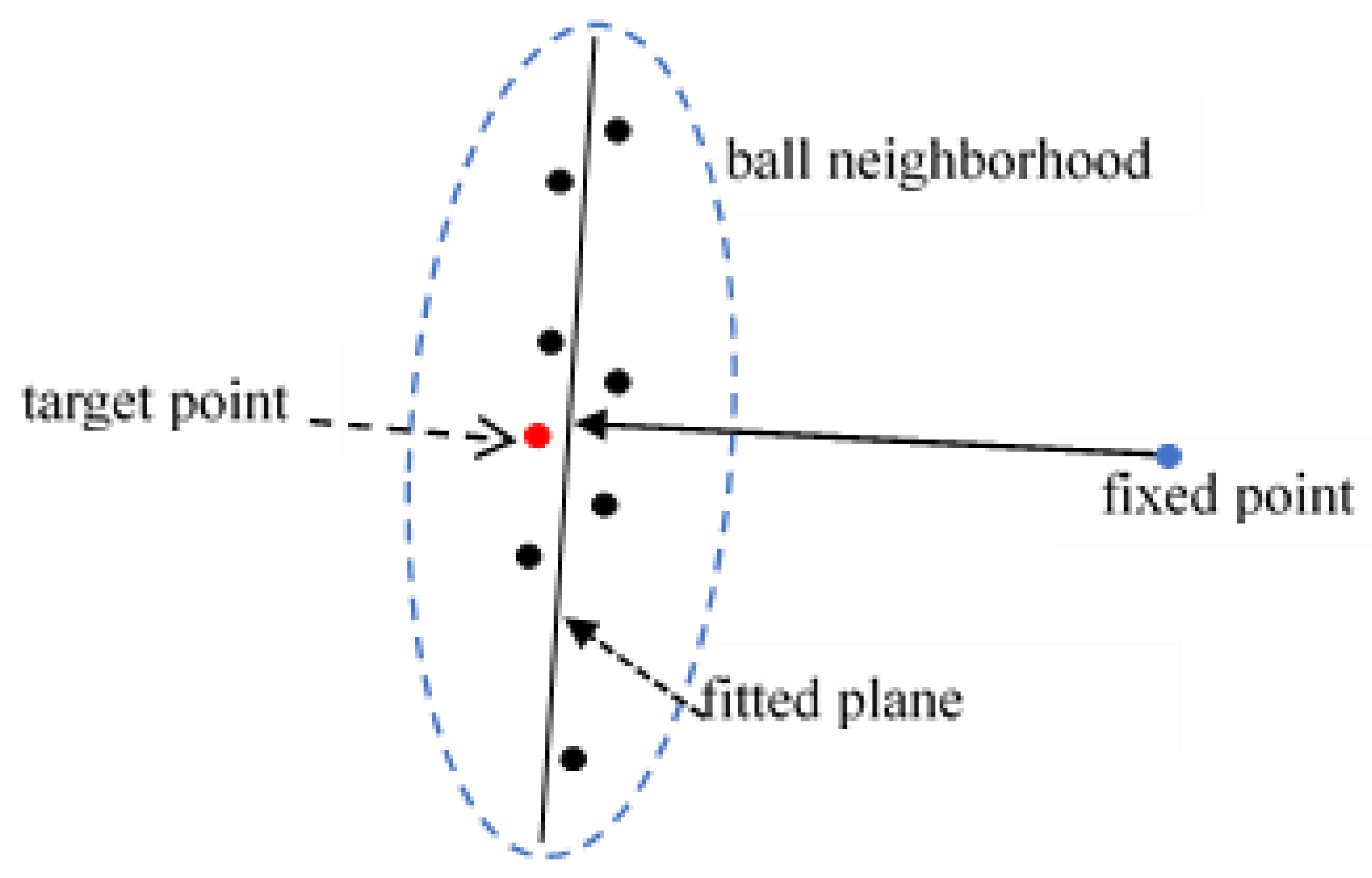
For a target point, first determine its local neighborhood points within a radius set by the user (in our case study, the radius is set as 0.02 m). Here we should demonstrate that the radius is determined closely related to the nominal size of the brick. In our case study, the nominal length, width, and height of the bricks are 0.10310 m, 0.05230 m and 0.03924 m, respectively. We tested the sensitivity of the radius, the results indicate that under the radius between 0.15 m and 0.25 m, the attribute space is distinguishable, that is, in the other application, the testing of the optimistic radius against the object size should be done, the value of which is neither too greater nor to small. Then, principle component analysis (PCA) is used to determine the surface normal of the neighborhood points as well as the plane equation [58].
A normal position vector was proposed to describe the point attributes in ref. [59]. Based on this, the geometry at the target point is determined by a spatial distance from a control point to the fitted plane around the target point. Here, control is a relative concept and the control point can be optionally specified as stated in ref. [59]. After fixing the control point, a position vector n from the control point to the plane fitted for a target point is defined and illustrated in Figure 5. The magnitude of the position vector | n | is the special distance, which is adopted as the geometrical attribute. It is assumed that the points belonging to the same plane have a similar magnitude of this special distance. Therefore, the special distance can be used to judge the planar patch. However, it may happen that different planes result in a similar special distance value, as illustrated in Figure 6: the distances from control point 1 to plane 1, plane 2 and plane 3 are all equal. Hence, it would be difficult to differentiate points belonging to different planes. In such a case, another control point 2 with drastically different distances, is introduced which avoids ambiguities in the special distance [59]. Figure 6 shows a situation where one control point is located at equal distance from two planes and the other control point is not. After two control points have been introduced, the magnitudes of distance from the first control point to the planes have the same attribute value (i.e., d 21 = d 22 = d 23 ), nevertheless, the magnitudes of the distances to the second control point to the planes are mutually different (i.e., d 21 d 22 d 23 ). Based on these properties, the points belonging to different planes are distinguished. Then, principle component analysis, PCA, is used to fit a plane and estimate the normal of that plane through the points in the neighborhood.
However, if one control point is located far away from the pile of bricks while the other control point is located inside the pile of bricks, the magnitude of the distances from each point to the two control points will have great difference. To illustrate, if the first control point is located 30 m from one brick while the second control point is located 1 m from the same brick, the attribute space for the first control point has poor recognition for different planes. This scale change will more or less influence the effectiveness of the planar segmentation implementation, which have not been considered in the previous works [59]. To avoid such scale change, the two control points are therefore always located inside point cloud. The location of the two control points is selected such that the two control points are well distributed meaning that the attributes of all points in the dataset will not have difference significantly. In our research, the positions of the two control points are determined as follows:
(1) calculate the minimum and maximum value for each coordinate of the 3D point cloud.
(2) estimate the 3D coordinates for the positions of the two control points (1 and 2) using Equation (3), see also in Figure 7.
c o n t r o l      p o i n t _ 1 = ( min X min    Y min    Z ) + 1 3 ( max X min X max Y min Y max Z min Z ) c o n t r o l      p o i n t _ 2 = ( min X min    Y min    Z ) + 2 3 ( max X min X max Y min Y max Z min Z )
Here min X and max X denote the minimum and maximum x-coordinates. min Y , max Y , min Z and max Z are defined similarly.
By using two control points, the likelihood of segmentation ambiguity is reduced. In general, the object space determined by an axis parallel bounding box. However, this cuboid might degenerate to a cube. In such situation, if the control points are located at the diagonal of the cube, the distances from the control points to the different faces of the cube are identical, as shown in Figure 7: Plane A and plane B have an equal distance to the first control point as well as to the second control point which means that plane A and plane B share the same location in attribute space. For removing such ambiguity thoroughly, the two control points should not be located on the diagonal of the cuboid. To optimize the locations, the two control points are shifted to the positions 1 and 2 , see Figure 7 (refer to the location introduced in ref. [59], the optimization is done). Here we should demonstrate that the positions of the control points are not unique as long as the ambiguity of location in the attribute space could be avoided. In the following, the 3D coordinates of the two control points are estimated by Equation (4).
C o o r d i n a t e s _ 1 = ( min X min    Y min    Z ) + ( 2 3 ( max X min X ) 1 3 ( max Y min Y ) 1 2 ( max Z min Z ) ) C o o r d i n a t e s _ 2 = ( min X min    Y min    Z ) + ( 1 2 ( max X min X ) 1 3 ( max Y min Y ) 2 3 ( max Z min Z ) )

3.4.2. Voting Scheme for Planar Segmentation

The attributes introduced in the last section are used to segment the points belonging to one plane. A voting scheme is used to obtain the segmentation. Voting schemes were proposed and applied in refs. [60,61,62]. The original idea is to extract implicit structural features in 3D point clouds affected by noise and isolated points. Voting schemes have been further developed given their significant inferential capability of structures and it has been applied for the detection of structural features in 3D point clouds [60,63,64]. In our research, it is used to segment the planar patches of bricks.
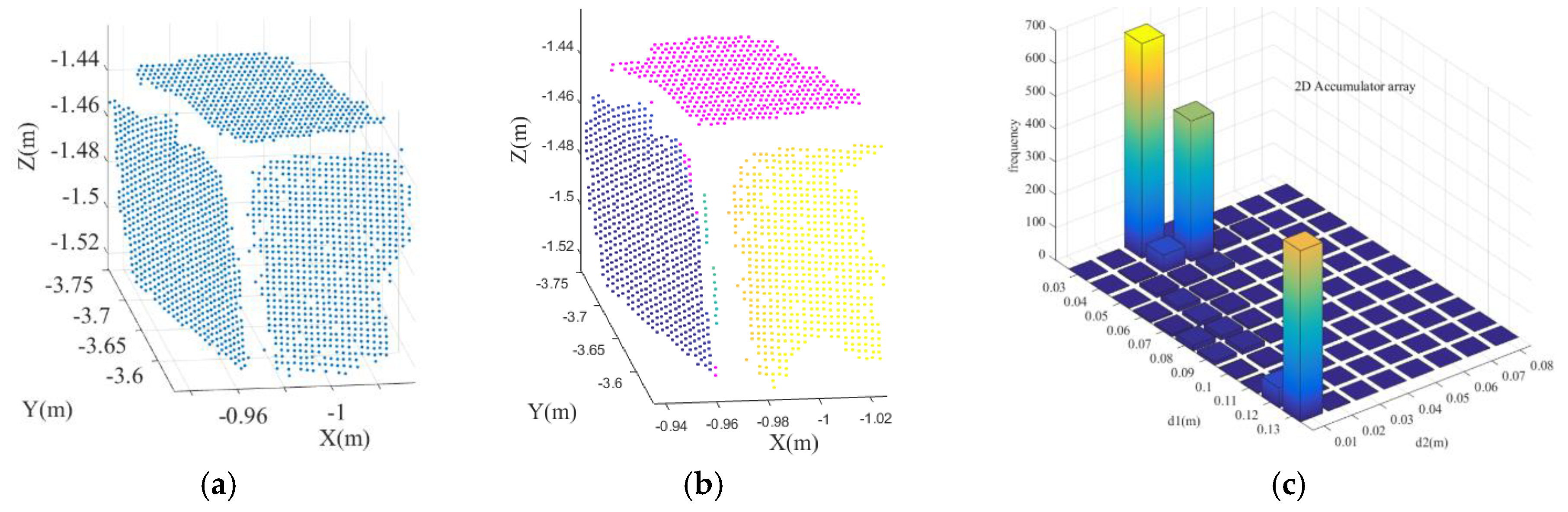
Note that the number of control points determines the dimension of the accumulator array, e.g., if one control point is selected for planar patch attribute computation, a one-dimensional accumulator array is adopted for the voting scheme. In our research, two control points are selected, therefore the accumulator array is two dimensional. As shown in Figure 6b, the accumulator array collects for each 3D point based on its two distances to the two control points. These two distances span the axis of the accumulator array. Next, the accumulator array is binned and the number of 3D points that contribute to each bin is counted. Here, a point cloud from one brick that includes three planar patches is selected to illustrate the voting scheme. For the points of this brick, the surface point density is about 1,200,000 pt / m 2 , as the point spacing is ~1 mm. To ensure that enough points are collected in the accumulators, the width is set as ten times the point spacing, i.e., 10 mm. Here we should demonstrate that the width is set by the user as long as the number of points collected in the accumulators is enough. In the following step (Section 3.4.3), the points will be refined clustered so that the value is not very crucial in the current step. Figure 8a shows the input point cloud. Through the voting scheme, three peaks are generated in the accumulator array, see Figure 8c. The points that belong to different planar patches after segmentation, are shown in Figure 8b in different colors.

3.4.3. Refined Clustering of Points

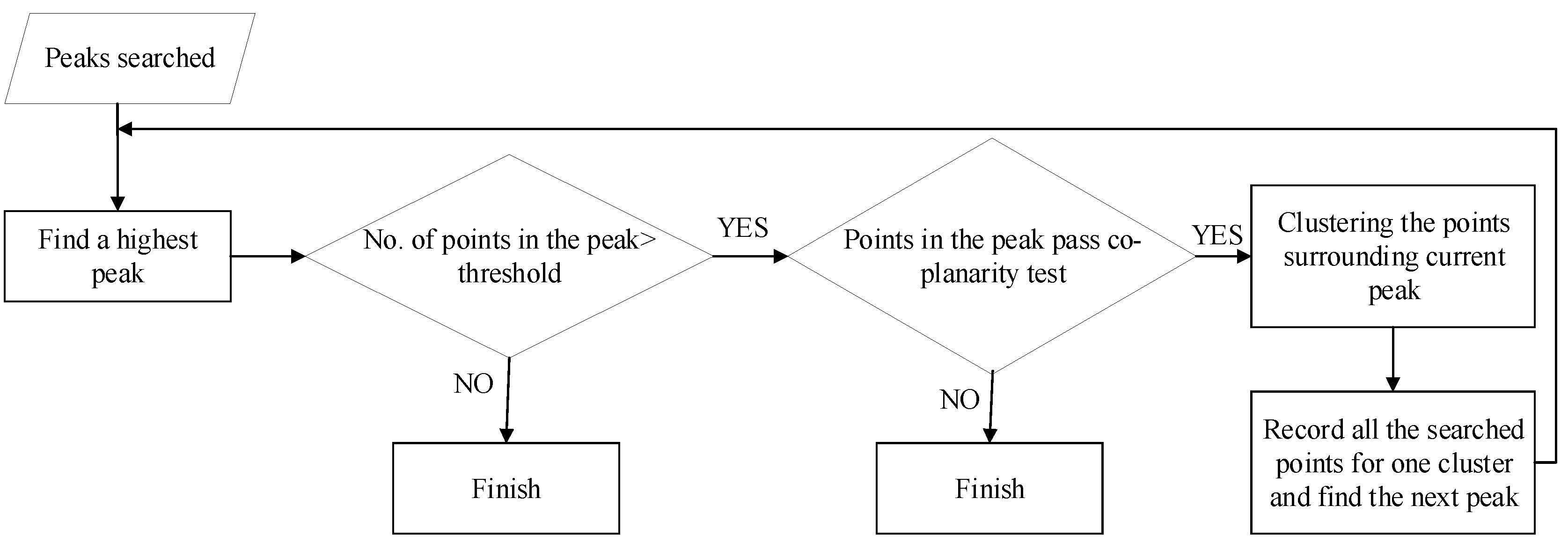
Once the locations of the two control points determined, the attributes (i.e., the special distance) for all points in the point cloud are estimated and recorded in the accumulator array. Afterwards, points with similar attributes (belonging to one planar patch) are clustered based on the points’ proximity and co-planarity. Points belonging to different planes in the object space are expected to form different peaks in the attribute space. Figure 9 illustrates the proposed flow of segmentation of points belonging to one planar patch.
In the process of segmentation, first a threshold is defined for the number of points in a peak that is expected to guarantee the composition of a planar patch, i.e., if the number of points in the peak is less than the threshold, the current peak will not be considered as a seed planar patch. Then, plane fitting is conducted using the points in the peak through PCA. Let the equation of the fitted plane be defined as Equation (5).
a x + b y + c z = d  
where the normal vector of the planar surface is defined as N = ( a , b , c ) and d is the distance of the plane to the origin.
Next, the distances d i of all points in the current peak to the fitted plane are calculated using Equation (6).
d i = | a x i + b y i + c z i d | a 2 + b 2 + c 2  
In which i = 1 , 2 , , n , n is the number of points in the current peak, d i is the distance for the i t h point in the current peak, ( x i , y i , z i ) denote the 3D coordinate for the i t h point.
Afterwards, the mean and RMS (Root Mean Square) of the distances are estimated as d and σ . The co-planarity of the points is evaluated by the RMS. More specifically, a fitting plane will be accepted when the RMS is less than the accuracy of the dataset. Once the points in the peak pass the co-planarity test, the points surrounding the current peak could be added to the fitted plane above using the distance. If the distance of points in a neighboring peak to the fitting plane satisfy d d j < σ ( j = 1 , 2 , , m , m is the number of points in the neighborhood peak), it is accepted as a point in the plane. In this way, all points in the current fitting plane are determined. Then, plane fitting using the points contributing to the current plane is conducted again by PCA and the obtained eigenvector with respect to the third component of PCA represents the final normal vector for the plane.

3.4.4. Planar Patches Merging and Clustering

The process introduced in Section 3.4.1, Section 3.4.2 and Section 3.4.3 is performed for all the components acquired in Section 3.3. In this way all possible planar patches are identified, as well as the corresponding centroid and normal vector. However, over-segmentation may occur induced by outliers and the sensitivity of the algorithm. Thus, the next step is to merge planar patches that have similar normals and low bias angles. Here, we use the centroid and the bias angle to realize this step, the core idea is to define a threshold for the centroid and the bias angle. Through comparing these two values, patches belonging to the same brick plane are found.
Afterwards, the process of clustering, i.e., finding the planar patches belonging to the same brick, is done based on the centroid, normal vector and the angle correlation. It should be noted that the normal vectors for the three patches belonging to one brick are mutually perpendicular. The process is first to search the planar patches within a defined centroids’ distance, then the planar patches belonging to one brick are found based on the induced angle between two planar patches within a defined angle value around π/2. To avoid faulty clustering, a threshold is fixed for the distance between the adjacent patches so that the maximum distance does not exceed this threshold. The idea to fix the threshold for the distance is based on the nominal size of the brick, i.e., if l 1 , l 2 and l 3 denote the nominal length, width and height of the brick respectively, the threshold could be expressed by ( l 1 / 2 ) 2 + ( l 2 / 2 ) 2 + Δ l . Here, l 1 l 2 l 3 and l 3 Δ l 0.01 m . In other words, it is better to set the distance threshold similar with the size of the brick; otherwise, it seems difficult to detect the planar patches.

3.5. Brick Reconstruction

Once all the planar patches are identified, the next step is to reconstruct the brick. Ideally, one brick consists of six planar patches of points, from which the brick could be reconstructed successfully. However, due to occlusions, scanning geometry and the accuracy of the clustering method, two issues exist in the processing. On one hand, the complete plane is hard to segment, i.e., only part of the points in the interior of the plane are extracted. However, the reconstruction uses the plane fitted on the detected points in one planar patch, so part of the points is enough for the fitting. In other words, complete planes are not required. On the other hand, it is practically impossible to acquire six planar patches for one brick. Generally, three perpendicular planar patches allow the reconstruction of a brick, as the intersection of the three planes enables to reconstruct the vertices of the brick. Once three planar patches are detected, the normal vector and the centroid of each planar patch are estimated, and their intersection is computed as well. Based on the three intersections, the first vertex of the brick is fixed. The next step is to reconstruct the other vertices. For some bricks, three surfaces could be scanned with fine scanning geometry. In many cases, however, maybe only two or one surfaces are scanned. When only one surface is scanned for one brick, it seems impossible to reconstruct the brick. A possible likely way is first to decide this surface belonging to which side of the brick based on its nominal length, width and height. Next step is to determine the brick direction in 3D space through combining the picture or the raw point cloud manually. Then the brick reconstruction could be done. However, considering that this process has uncertainty and needs manual work which results in the process is lack of automation and efficiency. Therefore, we do not consider this case in our research.
Below, the process of reconstructing the brick from two or three planar patches is introduced. In the case of three planar patches, once the first vertex, P 0 , is calculated and three normal vectors of the planar patches, v 1 , v 2 and v 3 , are estimated, a so-called brick coordinate system is defined as follows: the vertex P 0 is the origin of the brick coordinate system, v 1 , v 2 and v 3 are mutually perpendicular and parallel to the three axes of the brick coordinate system respectively, as shown in Figure 10: points C 1 , C 2 and C 3 denote the centroids of the plane A, B and C.
Within this special coordinate system, the other vertices are estimated. Here we take one vertex P 1 as example to illustrate the calculation procedure in detail. As shown in Figure 10, the first vertex P 0 and the centroid C 2 are represented as P 0 ( x P 0 , y P 0 , z P 0 ) and C 2 ( x C 0 , y C 0 , z C 0 ) respectively; the normal vector v 1 is v 1 ( a 1 , b 1 , c 1 ) . Thus, the vector P 0 C 2 ( x C 2 x P 0 , y C 2 y P 0 , z C 2 z P 0 ) projected to the direction of v 1 is given by Equation (7).
P 0 D 2 = P 0 C 2 v 1 v 1  
In practice, the normal vectors P 0 D 2 and D 2 P 1 are always identical. Therefore, the vector P 0 P 1 is determined as P 0 P 1 = 2 P 0 D 2 . In this way, the 3D coordinate of the vertex P 1 are easily obtained. Similarly, the 3D coordinates of the vertices P 3 and P 5 are estimated. Afterwards, the other vertices’ 3D coordinates are obtained based on the geometric attributes of the cuboid.
In the case of two planar patches, given that patches belonging to the same brick are mutually perpendicular and, thus, normal vectors associated to each facet should be perpendicular. Therefore, the normal vector for the third facet could be estimated. However, it seems there is no way to calculate any vertex for one brick because the centroid for the third facet is still unknown. Nevertheless, the nominal length ( a ), width ( b ) and height ( h ) can be used to obtain the coordinates of the vertex. As shown in Figure 10, three possible situations may occur: (1) Only patch A and patch B are segmented, (2) Only patch A and patch C are segmented, and (3) Only patch B and patch C are segmented. The process of reconstructing the brick is slightly different for each configuration. Here, the first situation is used as an example to illustrate the processing.
Only patch A and patch B are segmented. The process first estimates the centroids for the two patches ( C 1 and C 2 ). Next, six vertices, P 0 ~ P 5 , in the segmented planar patches, are estimated using the centroids and the principle components for the patches given by Equation (8).
P 0 = C 1 v 2 a / 2 v A 2 b / 2 P 1 = C 2 + v 1 h / 2 v B 1 b / 2 P 2 = C 2 + v 1 h / 2 + v B 1 b / 2 P 3 = C 1 v 2 a / 2 + v A 2 b / 2 P 4 = C 1 + v 2 a / 2 + v A 2 b / 2 P 5 = C 1 + v 2 a / 2 v A 2 b / 2
Here v A 2 is the second principle component for the points of patch A obtained by principle component analysis (PCA), v B 1 is the first principle component for the points of patch B, v 2 is the normal vector for patch B that is equal to the third principle component for the points of patch B. It should be noted that the PCA results depend on the number of points on each of the patches of the brick. However, the bricks in most cases are cuboids rather than cubic (faces are rectangles), and when the height and width of the brick are almost identical, it will be difficult to use the first or second components of the PCA for patch B. It is noteworthy that the normal vector ( v 2 ) of patch B is parallel to the first principle component ( v A 1 ) of the PCA of patch C while the first principle component ( v B 1 ) of the PCA of patch B is parallel to the normal vector ( v 3 ) of patch C. Thus, to solve the tricky of the first or second components of the PCA, the improvement of Equation (8) is done by the following replacement: v A 1 = v 2 and v 3 = v B 1 .
Once the vertices P 0 ~ P 5 are estimated, the vertices P 6 and P 7 are obtained according to the attributes of a cuboid as shown in Equation (9).
P 6 = P 1 + P 5 P 0 P 7 = P 2 + P 4 P 3

4. Results

4.1. Filter Needless Points Results

The first step is filtering of needless points. The points of two targets are easy to be recognized, and they are filtered manually by the user firstly. TLidar point cloud data were collected using a FARO LS-880 laser scanner, the nominal accuracy of which is ±3 mm (one sigma) as introduced in Section 2. Thus, the criterion for removing ground points is set as 6 mm. Combined with the normal vector for each point, the ground points were discarded coarsely. Next, the curvature for the remaining points was estimated by eigen value analysis of the local covariance matrix and vegetation points were removed. Finally, the local density was computed with a radius of 0.03 m for the remaining points. In this way, remaining outliers, vegetation points and ground points are filtered. The number of points in the raw point cloud is 1,514,123, and the number of left brick points is 258,876, i.e., a total number of filtered needless points is 1,255,247. The scatter diagram colored by Z value after the filtering results is shown in Figure 11. The remaining points are colored by Z value while removed points are colored by red. Note that, compared to manually removing the needless results, our method could implement in an automatic manner. On the other hand, the needless points close to the bricks are difficult to detect and remove manually. From the perspective of computational efficiency, though our method contains several steps, it is easy to implement based on the algorithms and methods proposed in previous articles.

4.2. Roughness Estimation Results

Afterwards, the roughness estimation for each point was completed in CloudCompare software (Paris, France) [55] according to the theory introduced in Section 3.2. In our study, parameter K was set at 50 to search nearest neighbors for the current point, and the least squares algorithm was implemented using the identified 50 points to fit a plane. Next, the distance representing the roughness was calculated from the current point to the fitted plane. Finally, the determined roughness values are in [0.000 0.025] m (In the symbol [], the left value is the minimum roughness while the right value is the maximum roughness). It is apparent that the points with relatively high roughness value are edge points and can be separated. Here, 0.0045 m as roughness threshold is selected for determining edge points. In other words, the points with a roughness values within the interval [0.0045 0.025] m are regarded as edge points. Figure 12 shows the scatter diagram colored by roughness for the remaining brick points. Note that, the roughness threshold determined here is related to the object shape and size, that is, for other applications, it has to be adjusted accordingly. Obviously, the greater the roughness threshold, the more points located at the edge of the bricks will be removed.

4.3. Coarse Segmentation Results

Once the edge points are removed, the 3D connected component analysis is implemented to segment brick points. The 3D grid step was set at 0.005 m which denotes the minimum gap between two components. The minimum number of points was set at 80 which means that components with less than 80 points will be ignored. In this way, the smallest components were removed automatically. The coarse segmentation results for the piles of bricks are shown Figure 13.
It should be noted that different bricks have various positions in the pile. Additionally, variation density and roughness induced by the scanning geometry inevitably happened. Those caused the coarse segmentation results (components) to include diverse situations that are classified in the following categories, see Figure 14: (a) less than three surface (one or two); (b) one brick, represented by three surfaces; (c) more than three surfaces. Therefore, further segmentation and grouping is required. In particular, searching for three surfaces belonging to one brick is a vital step for the brick reconstruction.

4.4. Planar Segmentation and Grouping Results

Next, the planar segmentation and clustering method introduced in Section 3.4 was implemented to work on individually components. In the process of computing the special distances to the two control points, a radius of 0.02 m was predefined for searching neighboring points. Then, the voting scheme and clustering of points were done for planar segmentation. As a result, all possible planar patches with their corresponding points were segmented. Figure 15a shows the segmentation result for the component in Figure 14c.
In Figure 15b, we can see that several brick planes were over segmented. It is required to further process such cases before reconstructing the bricks. In our study, the thresholds for the bias angle and the distance difference between the adjacent patches are set at one degree and 0.10 m. After merging the over segmented patches, patches were clustered, in which the induced angle between two planar patches in one brick was set equal to (π/2 ± π/180) and the centroid difference was set equal to 0.15 m. Figure 15b shows the clustering results for the same component. For each cluster, brick reconstruction was implemented, starting from the segmented planes, their centroids and corresponding normal vectors. The distance between the centroids of the planes, the angles between their normal vectors and the nominal length, width and height of the brick are used. In our experiment, the nominal length, width and height of the brick are obtained by measuring 4 complete brick point clouds, resulting in values of 0.10310 m, 0.05230 m and 0.03924 m, respectively. It should be noted that complete planes are not required for the reconstruction. See Figure 15b.

4.5. Reconstruction Results and Accuracy Assessment

The process is repeated with the remaining components until all detectable bricks are reconstructed. Figure 16a–d show the reconstruction results for four representative components. Figure 17 shows the reconstruction results for the whole piles of bricks, while the detected planar patches are plotted as well. Points for which no brick could be found are marked by a yellow ellipse. The number of bricks successfully reconstructed is 132, while the ground truth number is 175. Therefore, the completeness of the reconstruction result is about 75%. As we can see from Figure 17, bricks are in general reconstructed well. However, parts of bricks are sometimes missed in the reconstruction result, i.e., their planar patches could not be detected or the reconstruction process failed. Two main possible reasons for missing bricks are: (1) only one patch of one brick is scanned or detected; (2) the number of points in one patch is too small so that the true normal vector of the patch is hard to estimate.
One of the main interests of brick reconstruction is brick displacement estimation. For such application, the reconstruction accuracy needs to be ensured. To evaluate the accuracy, vertex points derived from automatic reconstruction are compared to points manually obtained from the raw point cloud using the Cloudcompare software (Paris, France) [55]. The accuracy is evaluated by the distance from the vertex manually obtained to the vertex computed by the proposed method. Vertices belonging to bricks only partly scanned are ignored, as we cannot pick the vertices manually. The histogram of the differences along x, y and z axes are plotted, see Figure 18a–c.
The number of vertices used in the accuracy assessment is 951. The mean difference values are 0.46, −0.36 and 0.34 mm along the x, y and z axes, respectively. The maximum difference values are 29.79, 29.74 and 29.68 mm along the x, y and z axes, respectively. Corresponding standard deviations are all below 10 mm with values of 9.66, 8.49 and 9.84 mm, respectively. It should be noted that only a small number of values are above 10 mm caused by scanning conditions such as occlusions, scanning geometry, et al., which results in no points or sparse points around brick corners. In other words, the vertices, picked manually with a significant difference values compared to reconstructed vertices, may not the ground truth values. In order to deepen the analysis of the accuracy, the vertices with an absolute difference value less than 10 mm are considered for further analysis, the number of which is 787 which means that about 83% of the vertices have a difference value of below 10 mm. The mean difference values, maximum difference values and standard deviations are calculated again for this subset. The mean difference values are −0.43, −0.70 and −1.00 mm along the x, y and z axes, respectively. The standard deviations are 4.55, 4.53 and 4.60 mm along the x, y and z axes, respectively. The standard deviations are relatively small which shows that the reconstruction accuracy is high from the position point of view. The accuracy assessment results are summarized in Table 1. Here, we should demonstrate that the mean difference values are expected to zero. However, brick fabrication is not perfect so that corners are often rounded instead of straight, see Figure 19, that is, the brick is not always a perfect cuboid. Considering that the magnitude of difference values is very small, the reconstructed results correspond well to reality. Furthermore, a successful workflow would profit from a carefully deigned measurement, which ensures that structural units (like bricks) are sampled well.

5. Discussion

5.1. Analysis of the Proposed Methodology

A methodology for segmenting and reconstructing bricks from a pile of bricks sampled by a terrestrial LiDAR point cloud is presented. In a automatic manner, the raw point cloud is first coarsely segmented into different components using 3D connected component analysis, then a voting scheme is used to segment planar patches. After refined clustering of points, merging and clustering patches, three or two patches belonging to one brick are searched and brick reconstruction is performed based on the geometry of a brick model, in which the nominal length, width and height are adopted as the essential parameters. The brick reconstruction is based on the identified planar patches (two or three) belonging to one brick. Through estimating the normal vectors using principle component analysis, the main, second and third components for a patch are determined, which combined with the nominal brick size, results in the brick vertices. Finally, to verify the accuracy of the proposed methodology, vertices are picked manually using the Cloudcompare software [55]. Here, the picking vertices are regarded as the ground true. The accuracy assessment results demonstrate that the proposed methodology for reconstructing bricks has good accuracy and can reconstruct vertices in a reliable way.
The proposed methodology provided a new way for further monitoring changes through comparing corresponding reconstructed bricks. In ref. [15], a method for the automatic extraction of face geometry of concrete cubic blocks that typically used in breakwaters was presented. Point clouds were segmented on the basis of their orientation and location, and through comparing corresponding cuboids the transformation parameters over time were estimated. Compared to this study, it is evident that the reconstructed bricks presented in this article for monitoring changes are much more intuitional. A methodology for the automatic modelling of breakwaters with armor units of cube shape was presented in ref. [14]. The accuracy of reconstructing the vertices was at centimeter level. Compared to this work, our methodology was proved to greatly improve the accuracy of reconstructing vertices, i.e., less than 5 mm along X, Y and Z axes, respectively. Furthermore, the size of cube (with a length of 1.25 m) presented in [14] is greater than the size of brick (with a length of 0.1 m) presented in this article, namely the brick is more complex to extract and reconstruct with respect to the cube. In this regard, the presented methodology here has better applicability for the brick-like structures with relatively small size. Besides this, it should be noted that the step of coarse segmentation of piles of bricks into small components using 3D component analysis simplified and accelerated the brick reconstruction procedures. To further assess the factors influencing the number of 75% accuracy, an experiment could be setup, where a pile is carefully constructed and scanned over and over again from different viewpoints, so that a more complete knowledge on the position of all individual bricks would be available.

5.2. Further Applications of the Proposed Methodology

The methodology presented here is an initial version using a dense point cloud acquired from a single scan position by terrestrial LiDAR. Considering a single scan may have avoided minor issues caused by registration, but the methodology in this paper is expected to work too for point clouds combining single scans. Dense point cloud data make it possible to extract almost all the brick surfaces and separate the individual bricks in a pile of bricks, which was not achieved previously in literature. Due to the inner characteristics of the 3D point cloud data, all the reconstructed bricks are located in its real position in 3D space, and subsequent change analysis or deformation analysis could be performed. Actually, many ancient masonry buildings that are composed of individual bricks, such as the Great Wall in China and Great Pyramid of Giza in Egypt, are still in service in modern society. In addition, the historical sites as related in ref. [41] are hot topics in archaeological engineering and their safety are of great importance. However, they suffer from aging effects, geo-hazards, urban construction, etc., thus it is necessary to analyze and detect changes from these structures. The presented methodology for separating and reconstructing the bricks could be a good ingredient to document masonry structures in a quantitative and accurate way. Furthermore, for the purpose of change detection, it can be extended to two situations:
(1) multiple scans from different positions in one epoch, in case larger scenes could be analyzed. In one scan, occlusions are unavoidable but occlusions can be largely avoided by using multiple scans. Meanwhile, for one brick, more planar patches will be scanned and segmented which will improve the accuracy and the efficiency of the brick reconstruction.
(2) multiple scans from the same position in different epochs, which would enable the brick change detection by comparing the corresponding bricks from different epochs. In this case, the point clouds from different epochs should be registered with high accuracy. Otherwise, small changes are difficult to identify due to alignment errors.

5.3. Future Work

The newly proposed methodology is an effective way of segmenting and reconstructing a large number of bricks sampled by terrestrial LiDAR point cloud that will enable applications on larger brick-like structures such as ancient walls, masonry churches, etc. For such applications, it is important that the components of a structure can be identified. However, the segmentation process is affected by variations in the point density, incident angle and point quality. Therefore, some manual processes are required for better segmentation results. In order to improve the applicability, some improvements can be made to enhance the process such as promote the adaptative to the point density, improve the performance of the noise reduction and the ability of extracting the boundary points. Furthermore, due to the limitations of the TLidar system that has varying performance induced by the variation in object range, object reflectivity and incident angle [65,66], it is better to set the system close to the structure, the value of which is determined by the size of the constitutional unit. The relationship between the ranges and the size of constitutional unit will be researched in future work.

6. Conclusions

This paper deals with a novel use of TLS applied to the 3D reconstruction of unorganized piles of bricks. The framework of segmenting and reconstructing the brick model is proposed and implemented. As part of the suitability assessment of the proposed methodology, an accuracy assessment by comparing the reconstructed vertices to the manually picked vertices was carried out. The results demonstrate the potential of dense TLS point cloud to reconstruct the objects with small size such as bricks and stones. The proposed methodology combines highly used algorithms, i.e., connected component analysis, principle component analysis and voting scheme, that enables the framework of our methodology to be highly transferable to data collected with other TLS instruments and similar scenarios. Furthermore, the detailed and high-precision brick model is of great value for post change detection and deformation analysis. This study provides new sights and references for the applications of TLS in segmenting and reconstructing individual objects from the scenarios composed by a large number of similar units such as masonry buildings, masonry bridges, rock slopes and high slopes.

Author Contributions

R.L. conceived and designed the experiments; Y.S. and R.L. developed the method; Y.S. and J.W. processed the dense point cloud data for individual bricks extraction; J.W. is Y.S.’s co-supervisor; V.G.F. helped polish the English; Y.S. wrote the original draft and all authors contributed in writing the paper.

Funding

This research was funded by the National Natural Science Foundation of China (grant number 41801379), National Key R&D Program of China (grant number 2016YFC0401801), the Fundamental Research Funds for the Central Universities (grant number 2018B58414) and Postdoctoral Science Foundation Funded Project of Jiangsu Province (grant number 2018K086C).

Acknowledgments

We would like to thank the China Scholar Council (CSC) for enabling Y.S. to study for one year at the Department of Geoscience and Remote Sensing, TU Delft. We gave thanks to the research group from the Department of Geoscience and Remote Sensing, TU Delft, for performing the experiment and conducting the field work. We also thank the anonymous reviewers and members of the editorial team for their comments and contributions.

Conflicts of Interest

The authors declare no conflict of interest.

References

  1. Cai, H.; Rasdorf, W. Modeling road centerlines and predicting lengths in 3-D using lidar point cloud and planimetric road centerline data. Comput. Aided Civ. Infrastruct. Eng. 2008, 23, 157–173. [Google Scholar] [CrossRef]
  2. Lehtomaki, M.; Jaakkola, A.; Hyypp, J.; Kukko, A.; Kaartinen, H. Detection of vertical pole-like objects in a road environment using vehicle-based laser scanning data. Remote Sens. 2010, 2, 641–664. [Google Scholar] [CrossRef]
  3. Shen, Y.; Lindenbergh, R.; Wang, J. Change analysis in structural laser scanning point clouds: The baseline method. Sensors 2017, 17, 26. [Google Scholar] [CrossRef] [PubMed]
  4. Ghuffar, S.; Szekely, B.; Roncat, A.; Pfeifer, N. Landslide displacement monitoring using 3D range flow on airborne and terrestrial lidar data. Remote Sens. 2013, 5, 2720–2745. [Google Scholar] [CrossRef]
  5. Kang, Z.; Zhang, L.; Lei, T.; Wang, B.; Chen, J. Continuous extraction of subway tunnel cross sections based on terrestrial point clouds. Remote Sens. 2014, 6, 857–879. [Google Scholar] [CrossRef]
  6. Kang, Z.; Zhang, L.; Yue, H.; Lindenbergh, R. Range image techniques for fast detection and quantification of changes in repeatedly scanned buildings. Photogramm. Eng. Remote Sens. 2013, 79, 695–707. [Google Scholar] [CrossRef]
  7. Kromer, R.A.; Abellán, A.; Hutchinson, D.J.; Lato, M.; Edwards, T.; Jaboyedoff, M. A 4D filtering and calibration technique for small-scale point cloud change detection with a terrestrial laser scanner. Remote Sens. 2015, 7, 16915–16916. [Google Scholar] [CrossRef]
  8. Barnhart, T.B.; Crosby, B.T. Comparing two methods of surface change detection on an evolving thermokarst using high-temporal-frequency terrestrial laser scanning, Selawik River, Alaska. Remote Sens. 2013, 5, 2813–2837. [Google Scholar] [CrossRef]
  9. Spina, S.; Debattista, K.; Bugeja, K.; Chalmers, A. Point cloud segmentation for cultural heritage sites. In Proceedings of the Vast 2011 The International Symposium on Virtual Reality, Archaeology and Intelligent Cultural Heritage, Prato, Italy, 18–21 October 2011; pp. 41–48. [Google Scholar]
  10. Rodriguez-Gonzalvez, P.; Munoz-Nieto, A.; Arias-Sanchez, P.; Gonzalez-Aguilera, D. Mobile lidar system: New possibilities for the documentation and dissemination of large cultural heritage sites. Remote Sens. 2017, 9, 189. [Google Scholar] [CrossRef]
  11. Xu, Z.; Wu, L.; Shen, Y.; Li, F.; Wang, Q.; Wang, R. Tridimensional reconstruction applied to cultural heritage with the use of camera-equipped uav and terrestrial laser scanner. Remote Sens. 2014, 6, 10413–10434. [Google Scholar] [CrossRef]
  12. Park, H.; Lee, H.; Adeli, H.; Lee, I. A new approach for health monitoring of structures: Terrestrial laser scanning. Comput. Aided Civ. Infrastruct. Eng. 2007, 22, 19–30. [Google Scholar] [CrossRef]
  13. Riveiro, B.; Dejong, M.J.; Conde, B. Automated processing of large point clouds for structural health monitoring of masonry arch bridges. Autom. Constr. 2016, 72, 258–268. [Google Scholar] [CrossRef]
  14. Bueno, M.; Diazvilarino, L.; Gonzalezjorge, H.; Martinezsanchez, J.; Arias, P. Automatic modelling of rubble mound breakwaters from lidar data. Int. Arch. Photogramm. Remote Sens. Spat. Inf. Sci. 2015, XL-3/W3, 9–13. [Google Scholar] [CrossRef]
  15. Puente, I.; Lindenbergh, R.; Gonzalez-Jorge, H.; Arias, P. Terrestrial laser scanning for geometry extraction and change monitoring of rubble mound breakwaters. ISPRS Ann. Photogramm. Remote Sens. Spat. Inf. Sci. 2014, 2, 289–294. [Google Scholar] [CrossRef]
  16. Corbi, H.; Riquelme, A.; Megias-Banos, C.; Abellan, A. 3-D morphological change analysis of a beach with seagrass berm using a terrestrial laser scanner. ISPRS Int. J. Geo-Inf. 2018, 7, 234. [Google Scholar] [CrossRef]
  17. Vosselman, G.; Maas, H.-G. Airborne and Terrestrial Laser Scanning; Whittles Publishing: Dunbeath, UK, 2010. [Google Scholar]
  18. Liu, Y.; Xiong, Y. Automatic segmentation of unorganized noisy point clouds based on the gaussian map. Comput. Aided Des. 2008, 40, 576–594. [Google Scholar] [CrossRef]
  19. Huang, J.; Menq, C.H. Automatic data segmentation for geometric feature extraction from unorganized 3-d coordinate points. IEEE Trans. Robot. Autom. 2001, 17, 268–279. [Google Scholar] [CrossRef]
  20. Wani, M.A.; Batchelor, B.G. Edge-region-based segmentation of range images. IEEE Trans. Pattern Anal. Mach. Intell. 1994, 16, 314–319. [Google Scholar] [CrossRef]
  21. Vo, A.V.; Truong-Hong, L.; Laefer, D.F.; Bertolotto, M. Octree-based region growing for point cloud segmentation. ISPRS J. Photogramm. Remote Sens. 2015, 104, 88–100. [Google Scholar] [CrossRef]
  22. Besl, P.J.; Jain, R.C. Segmentation through variable-order surface fitting. IEEE Trans. Pattern Anal. Mach. Intell. 2002, 10, 167–192. [Google Scholar] [CrossRef]
  23. Woo, H.; Kang, E.; Wang, S.; Lee, K.H. A new segmentation method for point cloud data. Int. J. Mach. Tools Manuf. 2002, 42, 167–178. [Google Scholar] [CrossRef]
  24. Lavoué, G.; Dupont, F.; Baskurt, A. A new cad mesh segmentation method, based on curvature tensor analysis. Comput. Aided Des. 2005, 37, 975–987. [Google Scholar] [CrossRef]
  25. Chen, Y.H.; Liu, C.Y. Quadric surface extraction using genetic algorithms. Comput. Aided Des. 1999, 31, 101–110. [Google Scholar] [CrossRef]
  26. Gotardo, P.F.U.; Bellon, O.R.P.; Boyer, K.L.; Silva, L. Range image segmentation into planar and quadric surfaces using an improved robust estimator and genetic algorithm. IEEE Trans. Syst. Man Cybern. Part B Cybern. 2004, 34, 2303–2316. [Google Scholar] [CrossRef]
  27. Johnson-Roberson, M.; Bohg, J.; BjoRkman, M.; Kragic, D. Attention-Based Active 3D Point Cloud Segmentation. In Proceedings of the IEEE/RSJ International Conference on Intelligent Robots and Systems, Taipei, Taiwan, 18–22 October 2010; pp. 1165–1170. [Google Scholar]
  28. Fujiwara, T.; Kamegawa, T.; Gofuku, A. Evaluation of plane detection with ransac according to density of 3D point clouds. Robotics, 2013; arXiv:1312.5033. [Google Scholar]
  29. Hulik, R.; Spanel, M.; Smrz, P.; Materna, Z. Continuous plane detection in point-cloud data based on 3D hough transform. J. Vis. Commun. Image Represent. 2014, 25, 86–97. [Google Scholar] [CrossRef]
  30. Camurri, M.; Vezzani, R.; Cucchiara, R. 3D hough transform for sphere recognition on point clouds. Mach. Vis. Appl. 2014, 25, 1877–1891. [Google Scholar] [CrossRef]
  31. Holz, D.; Behnke, S. Approximate triangulation and region growing for efficient segmentation and smoothing of range images. Robot. Auton. Syst. 2014, 62, 1282–1293. [Google Scholar] [CrossRef]
  32. Su, T.; Wang, W.; Lv, Z.; Wu, W.; Li, X. Rapid delaunay triangulation for randomly distributed point cloud data using adaptive hilbert curve. Comput. Graph. 2016, 54, 65–74. [Google Scholar] [CrossRef]
  33. Boissonnat, J.D. Geometric structures for three-dimensional shape representation. ACM Trans. Graph. 1984, 3, 266–286. [Google Scholar] [CrossRef] [Green Version]
  34. Xu, X.; Harada, K. Automatic surface reconstruction with alpha-shape method. Vis. Comput. 2003, 19, 431–443. [Google Scholar] [CrossRef]
  35. Gerschcnfeld, A.; Monianari, A. Reconstruction for models on random graphs. In Proceedings of the IEEE 48th Annual IEEE Symposium on Foundations of Computer Science (FOCS’07), Providence, RI, USA, 20–23 October 2007; pp. 194–204. [Google Scholar]
  36. Xiao, W.; Deng, M.; Li, C.; Liu, T. The study on point cloud data surface reconstruction based on power crust algorithm. Int. J. Digit. Content Technol. Appl. 2013, 7, 61–68. [Google Scholar]
  37. Hoppe, H.; DeRose, T.; Duchamp, T.; McDonald, J.; Stuetzle, W. Surface reconstruction from unorganized points. Comput. Graph. 1992, 26, 71–78. [Google Scholar] [CrossRef] [Green Version]
  38. Bernardini, F.; Mittleman, J.; Rushmeier, H.; Silva, C.; Taubin, G. The ball-pivoting algorithm for surface reconstruction. IEEE Trans. Vis. Comput. Graph. 1999, 5, 349–359. [Google Scholar] [CrossRef]
  39. Bodin, X.; Thibert, E.; Sanchez, O.; Rabatel, A.; Jaillet, S. Multi-annual kinematics of an active rock glacier quantified from very high-resolution dems: An application-case in the French Alps. Remote Sens. 2018, 10, 547. [Google Scholar] [CrossRef]
  40. Pradhan, B.; Fanos, A.M. Application of lidar in rockfall hazard assessment in tropical region. In Laser Scanning Applications in Landslide Assessment; Pradhan, B., Ed.; Springer International Publishing: Cham, Switzerland, 2017; pp. 323–359. [Google Scholar]
  41. Senol, H.I.; Erdogan, S.; Onal, M.; Ulukavak, M.; Memduhoglu, A.; Mutlu, S.; Ernst, F.B.; Yilmaz, M. 3D modeling of a bazaar in ancient harran city using laser scanning technique. ISPRS Int. Arch. Photogramm. Remote Sens. Spat. Inf. Sci. 2017, XLII-4/W6, 99–101. [Google Scholar] [CrossRef]
  42. Landa, J.; Prochazka, D.; Stastny, J. Point cloud processing for smart systems. Acta Univ. Agric. Silvic. Mendel. Brun. 2013, 61, 2415–2421. [Google Scholar] [CrossRef] [Green Version]
  43. Derron, M.H.; Metzger, R.; Carrea, D.; Jaboyedoff, M. Various approaches for vegetation filtering of terrestrial laser scans. In Proceedings of the EGU General Assembly Conference, Vienna, Austria, 22–27 April 2012. [Google Scholar]
  44. Little, A.V.; Maggioni, M.; Rosasco, L. Multiscale geometric methods for data sets I: Multiscale SVD, noise and curvature. Appl. Comput. Harmon. Anal. 2017, 43, 504–567. [Google Scholar] [CrossRef] [Green Version]
  45. Nurunnabi, A.; West, G.; Belton, D. Outlier detection and robust normal-curvature estimation in mobile laser scanning 3D point cloud data. Pattern Recognit. 2015, 48, 1404–1419. [Google Scholar] [CrossRef]
  46. Riquelme, A.J.; Abellan, A.; Tomas, R.; Jaboyedoff, M. A new approach for semi-automatic rock mass joints recognition from 3D point clouds. Comput. Geosci. 2014, 68, 38–52. [Google Scholar] [CrossRef] [Green Version]
  47. Connor, M.; Kumar, P. Fast construction of k-nearest neighbor graphs for point clouds. IEEE Trans. Vis. Comput. Graph. 2010, 16, 599–608. [Google Scholar] [CrossRef] [PubMed] [Green Version]
  48. Piegl, L.A.; Tiller, W. Algorithm for finding all k nearest neighbors. Comput. Aided Des. 2002, 34, 167–172. [Google Scholar] [CrossRef]
  49. Soudarissanane, S.; Lindenbergh, R.; Menenti, M.; Teunissen, P.J.G. Incidence angle influence on the quality of terrestrial laser scanning points. In Proceedings of the ISPRS Workshop Laser Scanning 2009, Paris, France, 1–2 September 2009; Volume 66, pp. 83–88. [Google Scholar]
  50. Dillencourt, M.B.; Samet, H.; Tamminen, M. A general approach to connected-component labeling for arbitrary image representations. J. ACM 1992, 39, 253–280. [Google Scholar] [CrossRef] [Green Version]
  51. Samet, H.; Tamminen, M. Efficient component labeling of images of arbitrary dimension represented by linear bintrees. IEEE Trans. Pattern Anal. Mach. Intell. 1988, 10, 579–586. [Google Scholar] [CrossRef]
  52. Nevalainen, O.; Honkavaara, E.; Tuominen, S.; Viljanen, N.; Hakala, T.; Yu, X.; Hyyppa, J.; Saari, H.; Polonen, I.; Imai, N. Individual tree detection and classification with uav-based photogrammetric point clouds and hyperspectral imaging. Remote Sens. 2017, 9, 185. [Google Scholar] [CrossRef]
  53. Borgefors, G.; Nystrom, I.; Di Baja, G.S. Connected components in 3D neighbourhoods. In Proceedings of the Scandinavian Conference on Image Analysis, Lappenranta, Finland, 9–11 June 1997; pp. 567–572. [Google Scholar]
  54. Zhang, J.; Duan, M.; Yan, Q.; Lin, X. Automatic vehicle extraction from airborne lidar data using an object-based point cloud analysis method. Remote Sens. 2014, 6, 8405–8423. [Google Scholar] [CrossRef]
  55. Girardeau-Montaut, D. Cloudcompare. 2017. Available online: http://www.cloudcompare.org/ (accessed on 19 December 2016).
  56. Osada, R.; Funkhouser, T.; Chazelle, B.; Dobkin, D. Shape distributions. ACM Trans. Graph. 2002, 21, 807–832. [Google Scholar] [CrossRef]
  57. Blomley, R.; Weinmann, M.; Leitloff, J.; Jutzi, B. Shape distribution features for point cloud analysis-a geometric histogram approach on multiple scales. ISPRS Ann. Photogramm. Remote Sens. Spat. Inf. Sci. 2014, 2, 9–16. [Google Scholar] [CrossRef]
  58. Awrangjeb, M.; Fraser, C. Automatic segmentation of raw lidar data for extraction of building roofs. Remote Sens. 2014, 6, 3716–3751. [Google Scholar] [CrossRef]
  59. Kim, C.; Habib, A.; Pyeon, M.; Kwon, G.; Jung, J.; Heo, J. Segmentation of planar surfaces from laser scanning data using the magnitude of normal position vector for adaptive neighborhoods. Sensors 2016, 16, 140. [Google Scholar] [CrossRef] [PubMed]
  60. Mordohai, P.; Medioni, G. Stereo using monocular cues within the tensor voting framework. IEEE Trans. Pattern Anal. Mach. Intell. 2006, 28, 968–982. [Google Scholar] [CrossRef] [PubMed]
  61. Medioni, G.; Tang, C.K.; Lee, M.S. Tensor voting: Theory and applications. In Proceedings of the Congrès Francophone Sur La Reconnaissance Des Formes et l’Intelligence Artificielle (RFIA), Paris, France, 1–3 Februaty 2000; Volume 34, pp. 1482–1495. [Google Scholar]
  62. Guy, G.; Medioni, G. Inference of surfaces, 3D curves, and junctions from sparse, noisy, 3D data. IEEE Trans. Pattern Anal. Mach. Intell. 1997, 19, 1265–1277. [Google Scholar] [CrossRef] [Green Version]
  63. Maggiori, E.; Lotito, P.; Manterola, H.L.; Del Fresno, M. Comments on “a closed-form solution to tensor voting: Theory and applications”. IEEE Trans. Pattern Anal. Mach. Intell. 2014, 36, 2567–2568. [Google Scholar] [CrossRef] [PubMed]
  64. Rui, F.; Moreno, P.; Bernardino, A. Robust cylinder detection and pose estimation using 3D point cloud information. In Proceedings of the IEEE International Conference on Autonomous Robot Systems and Competitions (ICARSC), Coimbra, Portugal, 26–28 April 2017; pp. 234–239. [Google Scholar]
  65. Tan, K.; Zhang, W.; Shen, F.; Cheng, X. Investigation of tls intensity data and distance measurement errors from target specular reflections. Remote Sens. 2018, 10, 1077. [Google Scholar] [CrossRef]
  66. Tan, K.; Cheng, X. Correction of incidence angle and distance effects on TLS intensity data based on reference targets. Remote Sens. 2016, 8, 251. [Google Scholar] [CrossRef]
Figure 1. Station view of the pile of bricks. Note that the targets have not been used in the work discussed in this paper. In addition, this work focuses on the extraction of bricks in the viewpoint of the scanner, not on the hidden bricks.
Remotesensing 10 01709 g001
Figure 2. Raw point cloud acquired by the FARO LS-880 Laser Scanner.
Remotesensing 10 01709 g002
Figure 3. Workflow for the brick segmentation and modelling.
Remotesensing 10 01709 g003
Figure 4. Workflow for plane recognition and grouping.
Remotesensing 10 01709 g004
Figure 5. Position vector illustrating the distance from the control point to a plane fitted using points neighboring a target point.
Remotesensing 10 01709 g005
Figure 6. Graphical illustration for the special distance using control points (cf. the graphical figure in [59]). (a) control point 1 is located at equal distance from three planes and for control point 2 distances to the three planes are different. (b) the distance from three planes to two control points.
Remotesensing 10 01709 g006
Figure 7. Location of the two control points.
Remotesensing 10 01709 g007
Figure 8. Voting scheme for the segmentation of points. (a) Input point cloud; (b) The segmented patches; (c) The 2D accumulator array.
Remotesensing 10 01709 g008
Figure 9. Work flow for the refined clustering of points.
Remotesensing 10 01709 g009
Figure 10. Graphical illustration for the brick reconstruction.
Remotesensing 10 01709 g010
Figure 11. Scatter diagram colored by Z value showing the filtering results.
Remotesensing 10 01709 g011
Figure 12. Scatter diagram colored by roughness value for the remaining brick points.
Remotesensing 10 01709 g012
Figure 13. Coarse segmentation results colored at random.
Remotesensing 10 01709 g013
Figure 14. Typical components for coarse segmentation. (a) Less than three surfaces (one or two); (b) Three surfaces; (c) More than three surfaces.
Remotesensing 10 01709 g014
Figure 15. Segmentation and reconstruction results for one component.
Remotesensing 10 01709 g015
Figure 16. Reconstruction examples for four representative components. (a) shows an example of components composing of one brick. (b) shows an example of components composing of more than five bricks. (c) shows an example of components composing of two bricks. (d) shows an example of components composing of five bricks.
Remotesensing 10 01709 g016
Figure 17. Reconstruction results for the entire piles of bricks.
Remotesensing 10 01709 g017
Figure 18. Histogram of the differences along x, y and z axes.
Remotesensing 10 01709 g018
Figure 19. A sketch illustrating that in practice brick corners are often rounded.
Remotesensing 10 01709 g019
Table 1. Accuracy assessment for the reconstruction.
TypeAxisMean Difference (mm)Maximum Difference (mm)Standard Deviation (mm)
Allx0.46 29.79 9.66
y−0.36 29.74 8.49
z0.34 29.68 9.84
Part (mean difference below 10 mm)x−0.43 9.94 4.55
y−0.70 9.87 4.53
z−1.00 9.92 4.60

