Article

Vegetation Indices Do Not Capture Forest Cover Variation in Upland Siberian Larch Forests

1
Department of Geography, Colgate University, Hamilton, NY 13346, USA
2
Northeast Science Station, Pacific Institute for Geography, Far East Branch, Russian Academy of Sciences, Cherskiy 678830, Russia
3
Department of Forestry, Forest and Wildlife Research Center, Mississippi State University, Starkville, MS 39759, USA
4
Center for Ecosystem Science and Society, Northern Arizona University, Flagstaff, AZ 86011, USA
5
Woods Hole Research Center, Falmouth, MA 02540, USA
*
Author to whom correspondence should be addressed.
Remote Sens. 2018, 10(11), 1686; https://doi.org/10.3390/rs10111686
Submission received: 21 September 2018 / Revised: 22 October 2018 / Accepted: 23 October 2018 / Published: 25 October 2018
(This article belongs to the Special Issue Optical Remote Sensing of Boreal Forests)

Abstract

:
Boreal forests are changing in response to climate, with potentially important feedbacks to regional and global climate through altered carbon cycle and albedo dynamics. These feedback processes will be affected by vegetation changes, and feedback strengths will largely rely on the spatial extent and timing of vegetation change. Satellite remote sensing is widely used to monitor vegetation dynamics, and vegetation indices (VIs) are frequently used to characterize spatial and temporal trends in vegetation productivity. In this study we combine field observations of larch forest cover across a 25 km2 upland landscape in northeastern Siberia with high-resolution satellite observations to determine how the Normalized Difference Vegetation Index (NDVI) and the Enhanced Vegetation Index (EVI) are related to forest cover. Across 46 forest stands ranging from 0% to 90% larch canopy cover, we find either no change, or declines in NDVI and EVI derived from PlanetScope CubeSat and Landsat data with increasing forest cover. In conjunction with field observations of NDVI, these results indicate that understory vegetation likely exerts a strong influence on vegetation indices in these ecosystems. This suggests that positive decadal trends in NDVI in Siberian larch forests may correspond primarily to increases in understory productivity, or even to declines in forest cover. Consequently, positive NDVI trends may be associated with declines in terrestrial carbon storage and increases in albedo, rather than increases in carbon storage and decreases in albedo that are commonly assumed. Moreover, it is also likely that important ecological changes such as large changes in forest density or variable forest regrowth after fire are not captured by long-term NDVI trends.

Graphical Abstract

1. Introduction

Boreal forest responses to warming temperatures will feed back to climate in a variety of important ways. Boreal ecosystems store globally significant amounts of terrestrial carbon in vegetation and soils. The balance between vegetation uptake and soil carbon losses is particularly important yet also represents a large source of uncertainty in high-latitude carbon cycle climate feedback, particularly in the context of permafrost thaw [1,2]. In addition to carbon cycle effects, vegetation change may also feed back to climate via altered ecosystem water and energy dynamics. Increases in evapotranspiration cool the land surface and increase atmospheric water vapor [3,4]. Increasing canopy cover reduces land surface albedo during the spring when vegetation masks snow, leading to surface warming [5]. When evergreen trees are replaced by deciduous species, by contrast, reductions in snow masking lead to increased albedo. Changes in light attenuation with canopy composition and density may also alter soil temperatures [6], which have important implications for soil carbon cycling. The magnitude of climate feedback associated with each of these processes depends on the rate and spatial extent of vegetation change. Consequently, there has been a great deal of effort to understand how boreal forest vegetation is responding to climate [7,8,9,10,11,12].
Optical remote sensing has emerged as one of the key tools used to understand ecosystem responses to climate. The existence of long-term satellite records such as the Advanced Very High Resolution Radiometer Global Inventory Modeling and Mapping Studies (AVHRR GIMMS) have enabled spatially and temporally continuous analyses of vegetation productivity that were among the first indications of biome-wide vegetation responses to climate [13]. Numerous Vegetation Indices (VIs) have been developed to use spectral information as a proxy for vegetation productivity, and the Normalized Difference Vegetation Index (NDVI) is the most commonly used VI. Long-term trends in NDVI are interpreted as increases or decreases in boreal forest productivity, and have been linked to tree growth and changes in forest composition [14]. However, comparison of multiple data sources that include products from new moderate resolution satellite sensors have revealed inconsistencies in NDVI trends [15,16]. Interpreting the ecological drivers of changes in NDVI is a key challenge for understanding high-latitude ecosystem responses to climate.
Recent increases in spatial and temporal resolution of satellite data, along with increases in computational efficiency are enabling investigation of spatial and temporal variation in high-latitude vegetation at finer scales. Landsat data with 30 m spatial resolution is increasingly being used to link the magnitude and direction of NDVI trends with different vegetation types [17,18] and to corroborate AVHRR trends [19]. Very high-resolution multispectral satellite data (i.e., <~4 m) from commercial platforms, such as IKONOS, QuickBird, and WorldView, provide even finer spatial detail and can be combined with historical aerial photographs to confirm hypothesized vegetation changes such as shrub and tree expansion into tundra [20], which in turn can be linked with NDVI trends [21]. Though very high-resolution satellite data has relatively poor temporal resolution, it has proven useful for mapping fine-scale variation in vegetation or ecosystem types and vegetation indices, primarily in tundra ecosystems [22,23,24,25]. Spatial relationships between vegetation properties and NDVI in Arctic tundra ecosystems are often used to support interpretations of temporal trends in NDVI [26]. To date there have been relatively few efforts to utilize very high-resolution vegetation indices and ecosystem properties as a tool to aid ecological interpretation of NDVI trends in boreal forests.
In this study we examine the effects of variability in forest cover on spatial and temporal variability in vegetation indices derived from very high-resolution multispectral satellite data with high temporal resolution. By comparing satellite data with field observations from boreal forests in Siberia that range from sparse to dense canopy cover we seek to answer the following questions: (1) Do values of commonly used vegetation indices increase with forest cover? and (2) Are there differences in overstory and understory phenology that correspond to differences in vegetation indices?

2. Materials and Methods

2.1. Study Site

The study was conducted along the Kolyma River in northeastern Siberia near the Northeast Science Station (NESS) located in the town of Cherskiy, Sakha Republic, Russia (68.74°N, 161.40°E). Mean annual, January, and July temperatures are −10 °C, −32 °C, and 13 °C, respectively, for the 1986–2015 period. Boreal forests in the area are composed exclusively of Larix cajanderi, a deciduous conifer hereafter referred to as larch. The understory is dominated by deciduous shrubs (Betula nana exilis, B. divaricata, Salix spp., and Vaccinium uliginosum), small evergreen shrubs (Vaccinium vitis-idaea, Empetrum nigrum, and Ledum decumbens (Ait.)), mosses (Aulacomnium turgidum, Dicranum spp., and Polytrichum spp.), and lichens (Cetraria spp. and Cladonia spp.). Forests of varying density are dominant in uplands to the east of the Kolyma River. Lowland floodplain ecosystems in the area contain forests but also large extensive shrublands dominated by Betula nana exilis, Salix spp., and Alnus fruticosa (Duschekia fruticosa), and also graminoid-dominated areas dominated by Eriophorum polystachion, Calamagrostis purpurea, and Carex spp. [27]. For this study, we examined a ~25 km2 area located to the east of NESS and the town of Cherskiy, as shown in Figure 1.

2.2. Field Data

We characterized tree density and canopy cover for 46 stands throughout the study area during the 2010–2017 field seasons [27,28]. There were no major disturbances or changes in land cover across the study area during this period. At each stand we established three 20 m long belt-transects spaced approximately 10 m apart that ranged from 1 to 4 m in width depending on tree density. Along each transect we recorded the number of stems and the diameter at breast height (DBH) for each stem. Existing allometric equations were used to calculate aboveground biomass from DBH, and multiplied by the proportion of carbon in live biomass (0.48) to determine aboveground larch biomass carbon content for each tree [27,28]. Larch canopy cover was measured using a hemispherical densitometer by taking four measurements in each cardinal direction at the beginning, middle, and end of each transect. Stand-level estimates for each variable were calculated as the mean of the three transects.
In June 2016 we installed in situ sensors to measure NDVI (SRS, Decagon Devices, Pullman WA, USA) at one high- and one low-density stand, as shown in Figure 2. At each stand, four downward facing sensors measured spectral radiance in the red (650 nm) and near infrared (810 nm) wavelengths. Of the four sensors at each stand, two were mounted at 7 m height on a tower mast above the larch canopy, and two were mounted below the larch canopy at 1 m above the ground surface. These downward facing sensors had a 36° field of view (fov) and were mounted at a 45° angle facing eastward and westward. In addition, three upward facing sensors with a 180° fov measured solar irradiance in the same red and near infrared wavelengths; one of these was mounted at 7 m height at the high-density site and the remaining two were mounted at 1 m height at the high- and low-density sites. Red and near infrared reflectance (R and NIR, respectively) were calculated by dividing radiance measured with the downward facing sensors by irradiance measured by collocated upward facing sensors. We assumed that the single upward facing sensor at 7 m was representative for both stands since they were located less than 2 km apart. We calculated NDVI for each of the eight downward facing sensors from R and NIR as follows:
N D V I = N I R R N I R + R
Measurements made at 60-s intervals were averaged every 30 min and recorded to a Decagon EM50 data logger. We used precipitation data from the Cherskiy airport to exclude data from days with rain. Mean NDVI values from 12:00 to 14:00 local time were used for analysis.
We observed phenology for overstory larch trees and understory shrubs (Betula and Salix) for the 2000–2017 time period across the landscape that included all of the study sites. We relied on visual observations made in forests near NESS because the phenophases described below occur rapidly and in concert across the study area. Start of the growing season (SOS) was defined as the timing of leaf emergence beginning with budburst and ending with leaf unfolding. This typically occurred rapidly over several days at the very end of May or the first half of June, and was followed by continued leaf growth through the end of June. End of the growing season (EOS) was defined as the visible onset of fall senescence as indicated by changes in leaf coloration (i.e., from green to yellow or red). This phenophase typically occurred rapidly over a period of several days in mid to late August. We defined SOS and EOS as the mid-point of the several day period over which leaf emergence and yellowing occurred, respectively. Growing season length (GSL) was defined as the difference between EOS and SOS.

2.3. Satellite Data

We utilized imagery from several satellite sensors to examine relationships between forest cover and VIs across the study area. To characterize forest cover across the study area we used a panchromatic WorldView2 image acquired on 8 March 2015. The 12-bit image had ~0.75 m spatial resolution and was converted to top-of-atmosphere (TOA) reflectance. This image was provided by the Polar Geospatial Center at the University of Minnesota (https://www.pgc.umn.edu/). To examine NDVI and EVI across the study area at high spatial and temporal resolution, we used data from the PlanetScope constellation of satellite sensors [29]. The PlanetScope constellation consists of approximately 120 CubeSats operated by Planet, a commercial satellite company. The PlanetScope satellites acquire imagery in four spectral bands (blue, green, red, and near infrared) with a ground sample distance (GSD) of 3–4 m. We used the Planet Surface Reflectance (SR) product collected using satellites deployed to a Sun-synchronous orbit, which is produced at 3 m spatial resolution and derived by first processing the Planet Analytic Radiance Product to TOA reflectance and then atmospherically correcting this to bottom-of-atmosphere or surface reflectance. Atmospheric corrections are preformed using the 6SV2.1 radiative transfer model [30] informed with atmospheric optical and water vapor information acquired from concurrent MODIS scenes. The Planet SR product does not account for haze or low cirrus clouds, so we manually screened images for clarity. In total, we utilized images acquired on 5 clear days between 15 June and 31 August 2017. We also used a single Landsat 8 OLI image for the study site acquired on 28 July 2017 to compare with the Planet SR data and to determine if relationships between VI and canopy cover were consistent between the two products. We acquired the Landsat Surface Reflectance Level-2 data product from the USGS EarthExplorer interface. We used the included quality band to mask clouds and cloud shadows from the Landsat image. Examination of the resulting NDVI image revealed that not all cloud shadows were excluded by the mask, so we used an NDVI threshold of 0.5 to further mask cloud shadows and anthropogenic surfaces. In addition to NDVI, we used the Enhanced Vegetation Index (EVI). EVI incorporates blue reflectance (B), in addition to the NIR and R, that helps to reduce impacts of the atmosphere and soil background [31]. We calculated EVI as follows:
E V I = 2.5 N I R R N I R + 6 R 7.5 B + 1

2.4. Data Analyses

We processed field data and satellite images, and performed all data analyses with R version 3.4.3 [32]. Manipulation and processing of geospatial data were performed using the Raster [33] and sp [34] packages in R. To compare field observations with satellite data, we used the geolocation of the center of the middle transect from each site, and then extracted data from all pixels within 15 m of the center point, except for Landsat data, where we used a single 30 m pixel.
To create maps of canopy cover, we developed a relationship between observed canopy cover and the 12-bit digital number representing TOA reflectance (DN) in the panchromatic image. DN values for each stand were determined by taking the mean of all pixels within 15 m of stand center. We standardized DN (DNS) values between 450 and 1000 to a range of 1–2 to avoid convergence issues when fitting an exponential model using the nls function in R. We fit an exponential model in the form of a*exp(-b*DNS) using data from all 46 stands and used the parameters with a map of DNS to create a map of canopy cover for the study area. We tested for significant differences between tree and shrub phenology metrics using a student’s t-test in R. To examine relationships between canopy cover and VIs we performed linear regression analyses using the lm function in R. All code used for analyses can be found at the following url: https://github.com/mloranty/ness_phenology/releases/tag/v2.0 [35].

3. Results

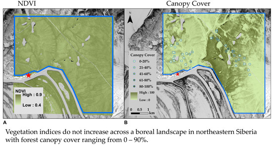
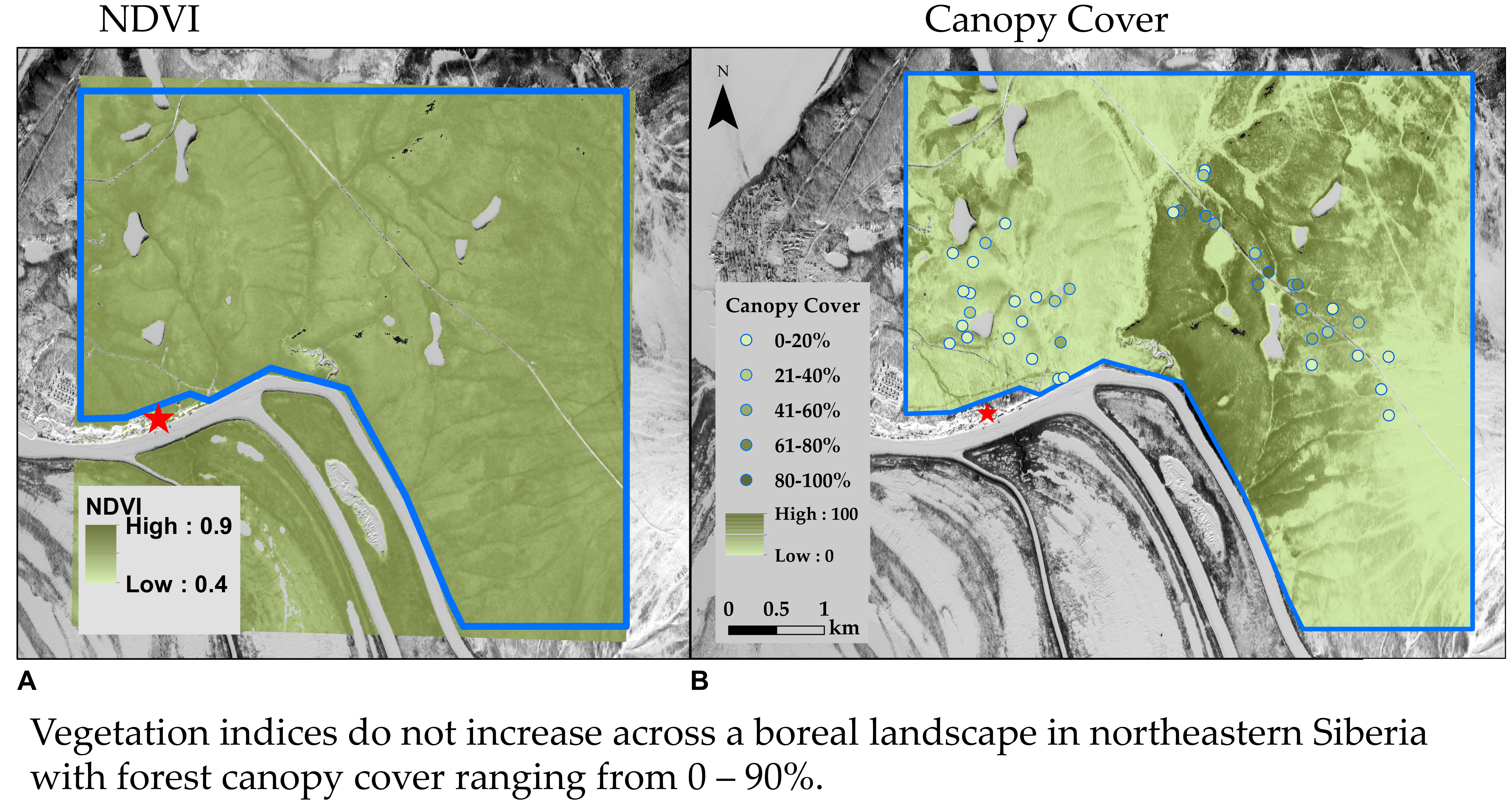
3.1. Landscape Spatial Variability in Vegetation Dynamics

Canopy cover ranged from 0% to 93% for the 46 stands sampled across the study area. Above ground larch biomass carbon ranged from 0 to 2750 g C m−2, and was closely linearly related with canopy cover, as shown in Figure 3, (r2 = 0.81, slope = 27.1, intercept = 37.5, p < 0.001). Canopy cover was inversely related to the standardized digital number for each stand (DNS) from the panchromatic satellite image, as shown in Figure 4 (a*exp(−b*DNS), a = 2560, b = 3.4, p < 0.001, RMSE = 14.1). We used this relationship to predict canopy cover across the study area, as shown in Figure 5. Mean predicted canopy cover for raster cells within a 15 m of stand center was closely correlated with observed values of canopy cover, as shown in Figure 6A (r2 = 0.69, slope = 0.71, intercept = 9.2, p < 0.001), and RMSE of predicted canopy cover for all stands was 14.1%. Residual canopy cover was inversely related to observed canopy cover, as shown in Figure 6B (r2 = 0.26, slope = −0.29, intercept = 9.2, p < 0.001), meaning that there was a tendency towards over-predictions at low canopy cover (<~20%) and under-predictions at high canopy cover (>~50%).
We observed differences in tree and shrub phenology across the study area, as shown in Table 1. Start of season (SOS) in larch occurred in the first week of June, on average three days before shrubs, but these differences were not significant, as shown in Table 1 (p = 0.1). End of season (EOS), indicated by onset of leaf senescence, occurred significantly later in larch (p < 0.01) with larch needles remaining green for an average of six days later in August than shrub leaves. On average, GSL was significantly longer by 8 days (p < 0.01) for larch trees than for the dominant understory shrubs.

3.2. Variability in NDVI

Field observations of NDVI displayed expected seasonal patterns, as shown in Figure 7. Maximum overstory NDVI ranged from 0.5 to 0.7 in 2016, as shown in Figure 7A, and 0.45 to 0.65 in 2017, as shown in Figure 7C, with differences of approximately 0.15 between east and west facing sensors at the low-density stand during the middle of the growing season, while within stand differences at the high-density stand were notably smaller, as shown in Figure 7A,C. At the low-density site understory NDVI values, as shown in Figure 7B,D, were similar to overstory values at both sites. Understory NDVI at the high-density site was notably lower than the low-density understory and displayed the least seasonal variability, as shown in Figure 7B,D.
Mean PlanetScope NDVI or EVI for each stand from five dates throughout the growing season, as shown in Figure 8A,B, was not positively related to observed canopy cover. The only statistically significant relationships between these vegetation indices and observed canopy cover were negative, and occurred late in the growing season. Mean growing season NDVI and EVI were negatively correlated with observed canopy cover, as shown in Figure 8C. Pixel-wise comparison of predicted tree cover with NDVI and EVI across the entire landscape yielded similar results, as shown in Figure 8D–F; the only significant relationships were negative associations between canopy cover and EVI late in the growing season. Landsat and PlanetScope exhibited similar geographic patterns in NDVI across the study area, as shown in Figure 9. Landsat NDVI was consistently higher than PlanetScope NDVI. Landsat NDVI was not significantly related to canopy cover, but Landsat EVI exhibited a significant negative correlation with canopy cover, as shown in Figure 10.

4. Discussion

4.1. What Drives Variability in Vegetation Indices?

NDVI and EVI did not increase appreciably with forest cover across a landscape with stands ranging from 0% to upwards of 90% canopy cover. The only significant relationships that we found were negative correlations between observed canopy cover and VIs late in the growing season, and when VIs were averaged across the growing season. Using modeled canopy cover across the entire landscape yielded the same results. The consistency of these results bolsters interpretation of analyses with modeled results, despite the inherent error associated with the relationship between DN and observed canopy cover. Moreover, given that the lowest VI values occurred in pixels with predicted canopy cover around 60%, and that the model was biased towards under-prediction at high canopy cover, these low VI values may actually represent areas with higher canopy cover. While PlanetScope VI values were consistently lower than Landsat, potentially due to wider spectral bands relative to Landsat [36] or differences in imaging geometry [37], geographic patterns and relationships between canopy cover and VIs were consistent across the two platforms.
Phenological differences between larch and the dominant understory shrubs were not clearly reflected in field or satellite VIs. If the phenological differences we observed contributed strongly to variation in VIs then areas with greater canopy cover should have had higher VI values during the start and end of the growing season because overstory trees green-up earlier and senesce later than dominant understory shrubs. However, mean growing season VIs were still lower in denser forests despite the fact that canopies there would have been green for longer than in low-density forests where understory plants contribute more to stand-wide measures of VIs. However, mean growing season VIs were inversely related to canopy cover. Despite the relatively high temporal resolution of PlanetScope data, we were not able to examine phenology differences during green-up or senescence, and the spatial distribution of our field measurements of NDVI were limited. Previous analyses have shown that seasonal NDVI dynamics are dominated by a combination of snow-melt as well as over- and under-story canopy phenology effects [38], and this is apparent in our 2017 field observations of NDVI. This may also be related to the fact that our phenology observations document changes in leaf coloration, but not senescence. Additionally, even 3 m pixels in all but the lowest and highest density stands likely contain a combination of overstory and understory reflectance. Further, Betula and Salix shrubs are only one component of understory vegetation communities in these ecosystems [27]. The presence of evergreen and non-vascular plants in the understory may dampen the phenological signal from trees and deciduous shrubs. These results highlight the difficulties of interpreting phenological metrics in Siberian larch forests with heterogeneous mixtures of needleleaf, broadleaf, and non-vascular plants with both deciduous and evergreen leaf habits.
Our field observations show that understory NDVI in low-density stands may exceed overstory NDVI, as shown in Figure 7, though these results should be interpreted with caution due to potential effects of different combinations of illumination and viewing geometry [37]. While the effect of understory vegetation has been recognized as an important factor influencing boreal forest reflectance [39], the relative invariance in VI across a large gradient in forest cover is unexpected. It may be the case that higher stem to leaf ratios in larch trees relative to understory vegetation components result in tree stems and branches having a strong negative effect on the VIs in high density forests. Lowland shrublands directly south across the river from NESS that were not included in our analyses had higher NDVI values than upland forested areas, as shown in Figure 9. Similarly, the dark dendritic features within the study area (i.e., high NDVI), as shown in Figure 9, are likely water tracks with dense tall shrub canopies. Broadleaf shrub canopies may mask the underlying woody plant components better than larch needles. In addition, other observations have shown a high degree of variability in understory reflectance [40] suggesting that variability in understory vegetation communities may contribute to spatial patterns in NDVI independently of overstory composition. Moreover, moss NDVI varies over short timescales with moisture conditions [41], which may help to explain daily and seasonal variability in understory NDVI observations, as shown in Figure 7B,D.

4.2. Implications for Interpreting NDVI Trends

Northeastern Siberia exhibits consistent greening trends across analyses of long-term NDVI data sets [15,42]. The magnitude of observed NDVI trends is relatively small in comparison to the range of NDVI values that we observed across a fairly large range of forest canopy cover and biomass values. Our observations are representative of forest cover across a much larger area [43] where 75% of the study regions had less than 1900 g m−2 in larch biomass. Seasonally integrated GIMMS NDVI is positively related to canopy cover across the 100,000 km2 Kolyma River watershed [9], however, this likely reflects geographic patterns in growing season length. On the other hand, tree ring indicators of larch growth were positively related to July NDVI [9], consistent with other analyses of larch growth and NDVI [44,45]. This may indicate that larch and understory vegetation are responding similarly to interannual climate variability, and that NDVI captures changes in ecosystem productivity in the absence of changes in forest cover.
While relationships between larch radial growth and NDVI trends indicate links between these two variables [44,45], our results illustrate the potential for relatively large increases in forest cover with no discernable NDVI response. Because larch density across this region is low [46], it is likely that NDVI trends are the result of combined understory and overstory responses to climate, or even dominated by understory responses. This highlights the need to separate overstory and understory spectral dynamics [47,48,49] in boreal larch forests. It is even possible that browning trends could result from increases in forest cover in these ecosystems. Indeed, the highest biomass stands in our study area are all approximately 50 years old, having originated from a stand-replacing fire that occurred approximately 80 years ago. The NDVI signal associated with this high biomass regrowth was most likely influenced by the vegetation communities preceding forest growth after fire. Our sites may also serve as useful treeline analogs because many of the understory species at our sites are common to tundra ecosystems as well. As such, our results indicate that ecotonal changes such as treeline advance may not be detected by NDVI trends.

5. Conclusions

We did not observe variation in NDVI or EVI across an upland boreal forest landscape in northeastern Siberia with forest canopy cover ranging from 0% to over 90%. Temporal differences in overstory and understory canopy phenology were not captured by satellite data, likely due to a lack of temporal resolution. Our results highlight the importance of understory vegetation in boreal VI dynamics, particularly in relation to interpretation of long-term trends. In these ecosystems, which dominate a large portion of boreal Siberia, invariant or declining NDVI and EVI with increasing forest cover highlights the potential for large changes in forest cover with no change in VIs. This is not unique to this region [50], but nonetheless poses a challenge for interpreting the potential climate feedback consequences associated with vegetation productivity trends inferred from NDVI in Siberian larch forests. Thus, long-term trends in satellite derived VIs must be interpreted with caution. Our results highlight the utility of high-resolution satellite data for understanding how VIs vary with ecosystem composition, and the continued need to investigate the contribution of understory vegetation to ecosystem VI dynamics.

Author Contributions

Conceptualization, M.M.L., H.D.A., S.M.N., M.C.M.; Methodology, M.M.L., and H.K.; Formal Analysis, M.M.L. and H.K.; Investigation, All Authors; Resources, S.P.D., and N.S.Z.; Data Curation, M.M.L. and H.K.; Writing-Original Draft Preparation, M.M.L.; Writing-Review & Editing, All Authors; Funding Acquisition, M.M.L., S.P.D., H.D.A., S.M.N., and M.C.M.

Funding

This research was funded by the National Geographic Society (9874-16, Loranty) and the National Science Foundation (PLR-1304040, PLR-1623764, PLR-1304007, PLR-1303940, Alexander, Loranty, Natali, Mack).

Acknowledgments

We thank numerous undergraduate and graduate research assistants, and Polaris Project participants for field and lab assistance. We thank the staff and scientists at the Northeast Science Station for logistical and field support. Lastly, we thank the editors and six anonymous reviewers whose comments helped to improve this paper.

Conflicts of Interest

The authors declare no conflict of interest. The founding sponsors had no role in the design of the study; in the collection, analyses, or interpretation of data; in the writing of the manuscript, and in the decision to publish the results.

References

  1. Abbott, B.W.; Jones, J.B.; Schuur, E.A.; Chapin, F.S., III; Bowden, W.B.; Bret-Harte, M.S.; Epstein, H.E.; Flannigan, M.D.; Harms, T.K.; Hollingsworth, T.N.; et al. Biomass offsets little or none of permafrost carbon release from soils, streams, and wildfire: an expert assessment. Environ. Res. Lett. 2016, 11, 1–13. [Google Scholar] [CrossRef]
  2. Welp, L.R.; Patra, P.K.; Rödenbeck, C.; Nemani, R.; Bi, J.; Piper, S.C.; Keeling, R.F. Increasing summer net CO 2 uptake in high northern ecosystems inferred from atmospheric inversions and comparisons to remote-sensing NDVI. Atmos. Chem. Phys. 2016, 16, 9047–9066. [Google Scholar] [CrossRef] [Green Version]
  3. Helbig, M.; Wischnewski, K.; Kljun, N.; Chasmer, L.E.; Quinton, W.L.; Detto, M.; Sonnentag, O. Regional atmospheric cooling and wetting effect of permafrost thaw-induced boreal forest loss. Glob. Chang. Biol. 2016, 22, 4048–4066. [Google Scholar] [CrossRef] [PubMed]
  4. Swann, A.L.; Fung, I.Y.; Levis, S.; Bonan, G.B.; Doney, S.C. Changes in Arctic vegetation amplify high-latitude warming through the greenhouse effect. Proc. Natl. Acad. Sci. USA 2010, 107, 1295–1300. [Google Scholar] [CrossRef] [PubMed] [Green Version]
  5. Loranty, M.M.; Berner, L.T.; Goetz, S.J.; Jin, Y.; Randerson, J.T. Vegetation controls on northern high latitude snow-albedo feedback: observations and CMIP5 model simulations. Glob. Chang. Biol. 2014, 20, 594–606. [Google Scholar] [CrossRef] [PubMed]
  6. Fisher, J.P.; Estop-Aragonés, C.; Thierry, A.; Charman, D.J.; Wolfe, S.A.; Hartley, I.P.; Murton, J.B.; Williams, M.; Phoenix, G.K. The influence of vegetation and soil characteristics on active-layer thickness of permafrost soils in boreal forest. Glob. Chang. Biol. 2016, 22, 3127–3140. [Google Scholar] [CrossRef] [PubMed] [Green Version]
  7. Soja, A.J.; Tchebakova, N.M.; French, N.H.; Flannigan, M.D.; Shugart, H.H.; Stocks, B.J.; Sukhinin, A.I.; Parfenova, E.I.; Chapin, F.S., III; Stackhouse, P.W., Jr. Climate-induced boreal forest change: Predictions versus current observations. Glob. Planet. Chang. 2007, 56, 274–296. [Google Scholar] [CrossRef] [Green Version]
  8. Tchebakova, N.; Parfenova, E.; Soja, A. The effects of climate, permafrost and fire on vegetation change in Siberia in a changing climate. Environ. Res. Lett. 2009, 4, 045013. [Google Scholar] [CrossRef] [Green Version]
  9. Berner, L.T.; Beck, P.S.A.; Bunn, A.G.; Goetz, S.J. Plant response to climate change along the forest-tundra ecotone in northeastern Siberia. Glob. Chang. Biol. 2013, 19, 3449–3462. [Google Scholar] [CrossRef] [PubMed]
  10. Bunn, AG. Observed and predicted responses of plant growth to climate across Canada. Geophys. Res. Lett. 2005, 32, 4. [Google Scholar] [CrossRef]
  11. Chapin, F.S., III; Callaghan, T.V.; Bergeron, Y.; Fukuda, M.; Johnstone, J.; Juday, G. Global change and the boreal forest: thresholds, shifting states or gradual change? AMBIO: J. Hum. Environ. 2004, 33, 361–365. [Google Scholar] [CrossRef]
  12. Chapin, F.S.; Mcguire, A.D.; Ruess, R.W.; Hollingsworth, T.N.; Mack, M.C.; Johnstone, J.F.; Kasischke, E.S.; Euskirchen, E.S.; Jones, J.B.; Jorgenson, M.T.; et al. Resilience of Alaska’s boreal forest to climatic change. Can. J. For. Res. 2010, 40, 1360–1370. [Google Scholar] [CrossRef]
  13. Myneni, R.; Keeling, C.; Tucker, C.; Asrar, G.; Nemani, R. Increased plant growth in the northern high latitudes from 1981 to 1991. Nature 1997, 386, 698–701. [Google Scholar] [CrossRef]
  14. Beck, P.S.; Juday, G.P.; Alix, C.; Barber, V.A.; Winslow, S.E.; Sousa, E.E.; Heiser, P.; Herriges, J.D.; Goetz, S.J. Changes in forest productivity across Alaska consistent with biome shift. Ecol. Lett. 2011, 14, 373–379. [Google Scholar] [CrossRef] [PubMed]
  15. Guay, K.C.; Beck, P.S.A.; Berner, L.T.; Goetz, S.J.; Baccini, A.; Buermann, W. Vegetation productivity patterns at high northern latitudes: a multi-sensor satellite data assessment. Glob. Chang. Biol. 2014, 20, 3147–3158. [Google Scholar] [CrossRef] [PubMed] [Green Version]
  16. Alcaraz-Segura, D.; Chuvieco, E.; Epstein, H.E.; Kasischke, E.S.; Trishchenko, A. Debating the greening vs. browning of the North American boreal forest: differences between satellite datasets. Glob. Chang. Biol. 2010, 16, 760–770. [Google Scholar] [CrossRef]
  17. McManus, K.M.; Morton, D.C.; Masek, J.G.; Wang, D.; Sexton, J.O.; Nagol, J.R.; Ropars, P.; Boudreau, S. Satellite-based evidence for shrub and graminoid tundra expansion in northern Quebec from 1986 to 2010. Glob. Chang. Biol. 2012, 18, 2313–2323. [Google Scholar] [CrossRef] [Green Version]
  18. Baird, R.A.; Verbyla, D.; Hollingsworth, T.N. Browning of the landscape of interior Alaska based on 1986-2009 Landsat sensor NDVI. Can. J. For. Res. 2012, 42, 1371–1382. [Google Scholar] [CrossRef]
  19. Ju, J.; Masek, J.G. The vegetation greenness trend in Canada and US Alaska from 1984–2012 Landsat data. Remote Sens. Environ. 2016, 176, 1–16. [Google Scholar] [CrossRef]
  20. Frost, G.V.; Epstein, H.E. Tall shrub and tree expansion in Siberian tundra ecotones since the 1960s. Glob. Chang. Biol. 2014, 20, 1264–1277. [Google Scholar] [CrossRef] [PubMed]
  21. Frost, G.V.; Epstein, H.E.; Walker, D.A. Regional and landscape-scale variability of Landsat-observed vegetation dynamics in northwest Siberian tundra. Environ. Res. Lett. 2014, 9, 025004. [Google Scholar] [CrossRef] [Green Version]
  22. Siewert, M.B.; Hanisch, J.; Weiss, N.; Kuhry, P.; Maximov, T.; Hugelius, G. Comparing carbon storage of Siberian tundra and taiga permafrost ecosystems at very high spatial resolution. J. Geophys. Res. Biogeosci. 2015, 120, 1973–1994. [Google Scholar] [CrossRef]
  23. Curasi, S.R.; Loranty, M.M.; Natali, S.M. Water track distribution and effects on carbon dioxide flux in an eastern Siberian upland tundra landscape. Environ. Res. Lett. 2016, 11, 1–12. [Google Scholar] [CrossRef]
  24. Mikola, J.T.; Virtanen, T.; Linkosalmi, M.; Vähä, E.; Nyman, J.; Postanogova, O.; Räsänen, T.A.; Kotze, D.J.; Laurila, T.; Juutinen, S.A.; et al. Spatial variation and linkages of soil and vegetation in the Siberian Arctic tundra – coupling field observations with remote sensing data. Biogeosciences 2018, 15, 2781–2801. [Google Scholar] [CrossRef] [Green Version]
  25. Juutinen, S.; Virtanen, T.; Kondratyev, V.; Laurila, T.; Linkosalmi, M.; Mikola, J.; Nyman, J.; Räsänen, A.; Tuovinen, J.P.; Aurela, M. Spatial variation and seasonal dynamics of leaf-area index in the arctic tundra-implications for linking ground observations and satellite images. Environ. Res. Lett. 2017, 12, 095002. [Google Scholar] [CrossRef] [Green Version]
  26. Walker, D.A.; Epstein, H.E.; Jia, G.J.; Balser, A.; Copass, C.; Edwards, E.J.; Gould, W.A.; Hollingsworth, J.; Knudson, J.; Maier, H.A. Phytomass, LAI, and NDVI in northern Alaska: Relationships to summer warmth, soil pH, plant functional types, and extrapolation to the circumpolar Arctic. J. Geophys. Res. Atmos. 2003, 108, 18. [Google Scholar] [CrossRef]
  27. Alexander, H.D.; Mack, M.C.; Goetz, S.; Loranty, M.M.; Beck, P.S.; Earl, K.; Zimov, S.; Davydov, S.; Thompson, C.C. Carbon Accumulation Patterns During Post-Fire Succession in Cajander Larch (Larix cajanderi) Forests of Siberia. Ecosystem 2012, 15, 1065–1082. [Google Scholar] [CrossRef] [Green Version]
  28. Webb, E.E.; Heard, K.; Natali, S.M.; Bunn, A.G.; Alexander, H.D.; Berner, L.T.; Kholodov, A.; Loranty, M.M.; Schade, J.D.; Spektor, V. Variability in above- and belowground carbon stocks in a Siberian larch watershed. Biogeosciences 2017, 14, 4279–4294. [Google Scholar] [CrossRef] [Green Version]
  29. Planet Team. Planet Application Program Interface: In Space for Life on Earth. [Internet]. San Francisco, CA, 2017. Available online: https://api.planet.com (accessed on 19 August 2018).
  30. Vermote, E.F.; Tanre, D.; Deuze, J.L.; Herman, M.; Morcette, J.J. Second Simulation of the Satellite Signal in the Solar Spectrum, 6S: An overview. IEEE Trans. Geosci. Remote Sens. 1997, 35, 675–686. [Google Scholar] [CrossRef]
  31. Huete, A.; Didan, K.; Miura, T.; Rodriguez, E.; Gao, X.; Ferreira, L.G. Overview of the radiometric and biophysical performance of the MODIS vegetation indices. Remote Sens. Environ. 2002, 83, 195–213. [Google Scholar] [CrossRef]
  32. R Development Core Team. R: A Language and Environment for Statistical Computing; R Foundation for Statistical Computing: Vienna, Austria, 2014; Available online: http://www.R-project.org/ (accessed on 25 October 2018).
  33. Hijmans, R. Raster: Geographic Analysis and Modeling with Raster Data, 2nd ed.; R Foundation for Statistical Computing: Vienna, Austria; pp. 1–204. Available online: https://CRAN.R-project.org/package=raster (accessed on 25 October 2018).
  34. Pebesma, E.; Bivand, R.S. Classes and methods for spatial data: the sp Package. R News 2005, 5, 9–13. [Google Scholar]
  35. Loranty, M. NESS NDVI and Phenology Data and Code. GitHUB Repository v2.0. , 2018. Available online: https://github.com/mloranty/ness_phenology/releases/tag/v2.0, doi.org.10.5281/zenodo.1468054 (accessed on 25 October 2018).
  36. Houborg, R.; McCabe, M.F. A Cubesat enabled Spatio-Temporal Enhancement Method (CESTEM) utilizing Planet, Landsat and MODIS data. Remote Sens. Environ. 2018, 209, 211–226. [Google Scholar] [CrossRef]
  37. Bhandari, S.; Phinn, S.; Gill, T. Assessing viewing and illumination geometry effects on the MODIS vegetation index (MOD13Q1) time series: implications for monitoring phenology and disturbances in forest communities in Queensland, Australia. Int. J. Remote Sens. 2011, 32, 7513–7538. [Google Scholar] [CrossRef]
  38. Suzuki, R.; Kobayashi, H.; Delbart, N.; Asanuma, J.; Hiyama, T. NDVI responses to the forest canopy and floor from spring to summer observed by airborne spectrometer in eastern Siberia. Remote Sens. Environ. 2011, 115, 3615–3624. [Google Scholar] [CrossRef]
  39. Chen, J.M.; Cihlar, J. Retrieving leaf area index of boreal conifer forests using Landsat TM images. Remote Sens. Environ. 1996, 55, 153–162. [Google Scholar] [CrossRef]
  40. Rautiainen, M.; Mottus, M.; Heiskanen, J.; Akujärvi, A.; Majasalmi, T.; Stenberg, P. Seasonal reflectance dynamics of common understory types in a northern European boreal forest. Remote Sens. Environ. 2011, 115, 3020–3028. [Google Scholar] [CrossRef]
  41. May, J.L.; Parker, T.; Unger, S.; Oberbauer, S.F. Short term changes in moisture content drive strong changes in Normalized Difference Vegetation Index and gross primary productivity in four Arctic moss communities. Remote Sens. Environ. 2018, 212, 114–120. [Google Scholar] [CrossRef]
  42. Beck, P.S.A.; Goetz, S.J. Satellite observations of high northern latitude vegetation productivity changes between 1982 and 2008: ecological variability and regional differences. Environ. Res. Lett. 2011, 6, 045501. [Google Scholar] [CrossRef] [Green Version]
  43. Berner, L.T.; Beck, P.S.A.; Loranty, M.M.; Alexander, H.D.; Mack, M.C.; Goetz, S.J. Cajander larch (Larix cajanderi) biomass distribution, fire regime and post-fire recovery in northeastern Siberia. Biogeosciences 2012, 9, 3943–3959. [Google Scholar] [CrossRef]
  44. Lloyd, A.H.; Bunn, A.G.; BERNER, L. A latitudinal gradient in tree growth response to climate warming in the Siberian taiga. Glob. Chang. Biol. 2010, 17, 1935–1945. [Google Scholar] [CrossRef]
  45. Bunn, A.G.; Hughes, M.K.; Kirdyanov, A.V.; Losleben, M.; Shishov, V.V.; Berner, L.T.; Oltchev, A.; Vaganov, E.A. Comparing forest measurements from tree rings and a space-based index of vegetation activity in Siberia. Environ. Res. Lett. 2013, 8, 035034. [Google Scholar] [CrossRef] [Green Version]
  46. Loranty, M.M.; Lieberman-Cribbin, W.; Berner, L.T.; Natali, S.M.; Goetz, S.J.; Alexander, H.D.; Kholodov, A.L. Spatial variation in vegetation productivity trends, fire disturbance, and soil carbon across arctic-boreal permafrost ecosystems. Environ. Res. Lett. 2016, 11, 1–13. [Google Scholar] [CrossRef]
  47. Lu, H.; Raupach, M.R.; McVicar, T.R.; Barrett, D.J. Decomposition of vegetation cover into woody and herbaceous components using AVHRR NDVI time series. Remote Sens. Environ. 2003, 86, 1–18. [Google Scholar] [CrossRef]
  48. Pisek, J.; Rautiainen, M.; Heiskanen, J.; Mottus, M. Retrieval of seasonal dynamics of forest understory reflectance in a Northern European boreal forest from MODIS BRDF data. Remote Sens. Environ. 2012, 117, 464–468. [Google Scholar] [CrossRef]
  49. Pisek, J.; Chen, J.M.; Kobayashi, H.; Rautiainen, M.; Schaepman, M.E.; Karnieli, A.; Sprintsin, M.; Ryu, Y.; Nikopensius, M.; Raabe, K. Retrieval of seasonal dynamics of forest understory reflectance from semiarid to boreal forests using MODIS BRDF data. J. Geophys. Res. Biogeosci. 2016, 121, 855–863. [Google Scholar] [CrossRef]
  50. Verbesselt, J.; Hyndman, R.; Newnham, G.; Culvenor, D. Detecting trend and seasonal changes in satellite image time series. Remote Sens. Environ. 2010, 114, 106–115. [Google Scholar] [CrossRef]
Figure 1. Map of the study area in northeastern Siberia. The blue polygon denotes the upland larch forested area used for analysis in this study. The red star denotes the location of the Northeast Science Station. Colored points indicate forest stand sample locations and associated canopy cover values. The background image is a panchromatic WorldView2 satellite image from 8 March 2015.
Remotesensing 10 01686 g001
Figure 2. Aerial photographs of the high-density (A) and low-density (B) stands instrumented for in situ Normalized Difference Vegetation Index (NDVI). Photographs were both taken during leaf-out on 1 June 2017. Tower masts are located in the upper right corner of the photographs. Photographs: M. Loranty.
Remotesensing 10 01686 g002
Figure 3. Linear relationship between canopy cover and aboveground larch biomass carbon for 46 stands sampled across an upland landscape. Whiskers indicate standard error of the mean (SE).
Remotesensing 10 01686 g003
Figure 4. Inverse non-linear relationship between stand-level canopy cover and digital number (DN) from a March 2015 panchromatic WorldView2 image. Note the model was fit using standardized digital numbers (DNS) and data were back-transformed for plotting. Vertical whiskers indicate standard error (SE) of mean canopy cover, and horizontal whiskers are one standard deviation (SD) of mean stand DN.
Remotesensing 10 01686 g004
Figure 5. Map of canopy cover across the study area predicted using the relationship between DN and field observations shown in Figure 4.
Remotesensing 10 01686 g005
Figure 6. Relationship between observed and predicted canopy cover (A), and between observed and residual canopy cover (B). Dashed lines show regression fits, thin solid lines indicate 1:1 lines (A), and abscissa (B).
Remotesensing 10 01686 g006
Figure 7. Field observations of NDVI from overstory (A) and understory (B) sensors for 2016, and from overstory (C) and understory (D) sensors in 2017. Blue and black symbols represent measurements from the low- and high-density stands, respectively. Open and closed circles indicate replicate (east- and west-facing) sensors at each stand. Points represent daily observations and lines are a 5-day running mean.
Remotesensing 10 01686 g007
Figure 8. Relationships between observed canopy cover and PlanetScope NDVI (A) and EVI (B) across all 46 forest stands for five days during the growing season, and also for both indices averaged across the growing season (C). Plot whiskers show the standard error of mean observed canopy cover, and the standard deviation of NDVI/EVI for all pixels with centers located within 15 m of the stand center. Plots (DF) show the same, but with modeled canopy cover aggregated into bins of 10%. Shaded polygons represent the standard deviation of NDVI/EVI within each canopy cover bin. In all plots, trend lines show significant (p < 0.05) linear relationships between canopy cover and NDVI/EVI. Absence of trendlines indicates no significant relationship.
Remotesensing 10 01686 g008
Figure 9. NDVI maps across the study area from PlanetScope on 26 July 2017 (A) and Landsat on 28 July 2017 (B). Note the maps use the same scale, indicating that Landsat has higher NDVI values than PlanetScope.
Remotesensing 10 01686 g009
Figure 10. Relationships between Landsat Vegetation Indices (VI) from 28 July 2017 image and observed canopy cover. Dashed lines show statistically significant relationship (p < 0.05). Horizontal whiskers indicate standard error (SE) of mean canopy cover.
Remotesensing 10 01686 g010
Table 1. Phenology differences between overstory larch trees and understory Betula and Salix shrubs for the 2000–2017 period. Values in parentheses represent one standard deviation.
SOSEOSGSL
Larch153 (4)240 (4) a87 (6) b
Shrub156 (5)234 (4) a79 (7) b
a significantly different at p < 0.01; b significantly different at p < 0.01. SOS: Start of season; EOS: End of season; GSL: Growing season length.

