Figure 1.
Korea Ministry of Environment (KME) land cover map of South Korea with 5 m spatial resolution (
http://www.me.go.kr/eng/web/main.do). The red circles indicate counties with more than 5000 ha of paddy areas, according to data obtained from the Korean Statistical Information Service (KOSIS) for the calibration of the crop model.
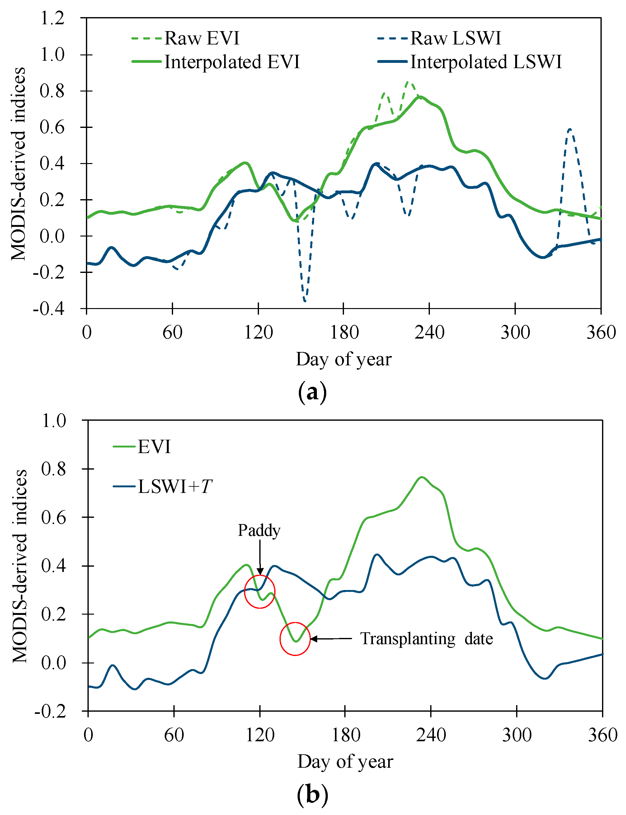
Figure 2.
Seasonal variations in enhanced vegetation index (EVI) and land surface water index (LSWI) derived from Moderate Resolution Imaging Spectroradiometer (MODIS) imagery at a paddy field in South Korea: (a) comparisons between raw and interpolated indices (EVI and LSWI) and (b) conditions for the detection of paddy fields and transplanting date. T is the threshold value of the LSWI.
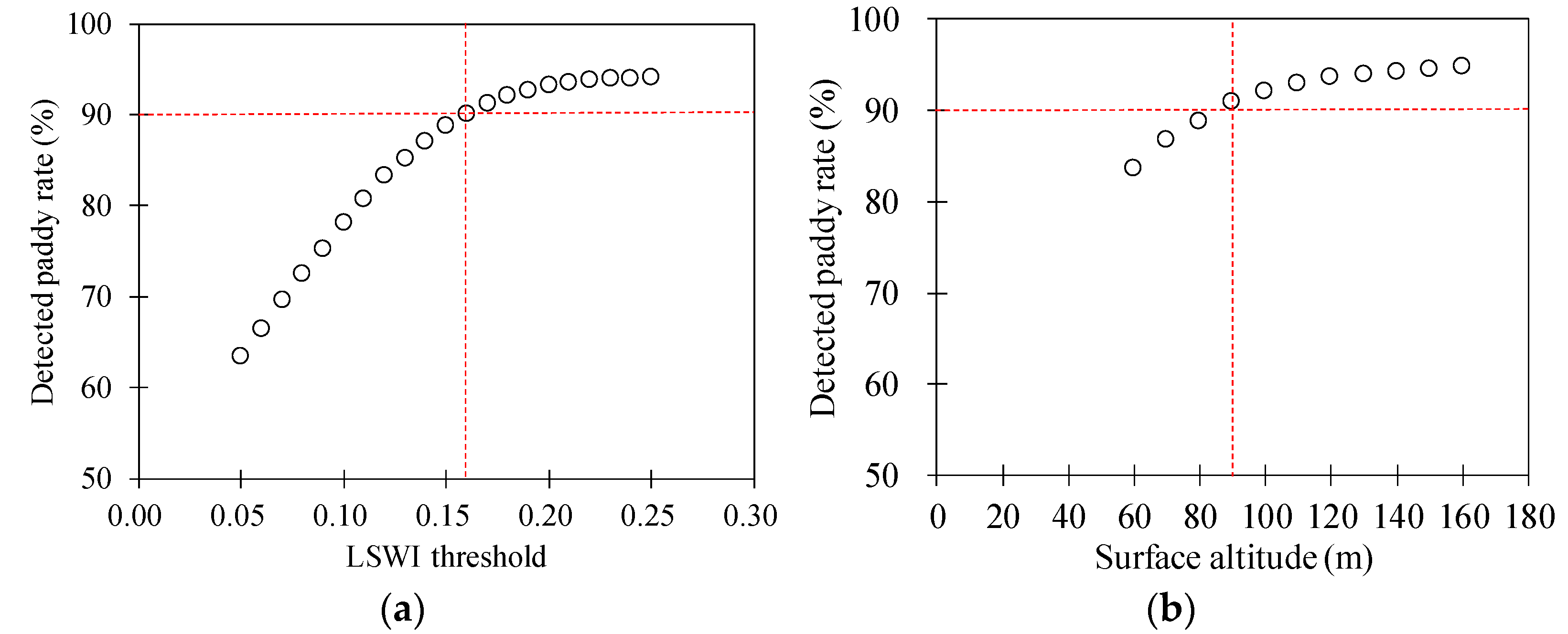
Figure 3.
Determination of the thresholds as functions of (a) land surface water index (LSWI), (b) surface altitude, and (c) surface slope used to detect paddy fields. The red dotted lines show the determined threshold values when the detected paddy rates exceed 90% while increasing the threshold values at regular intervals.
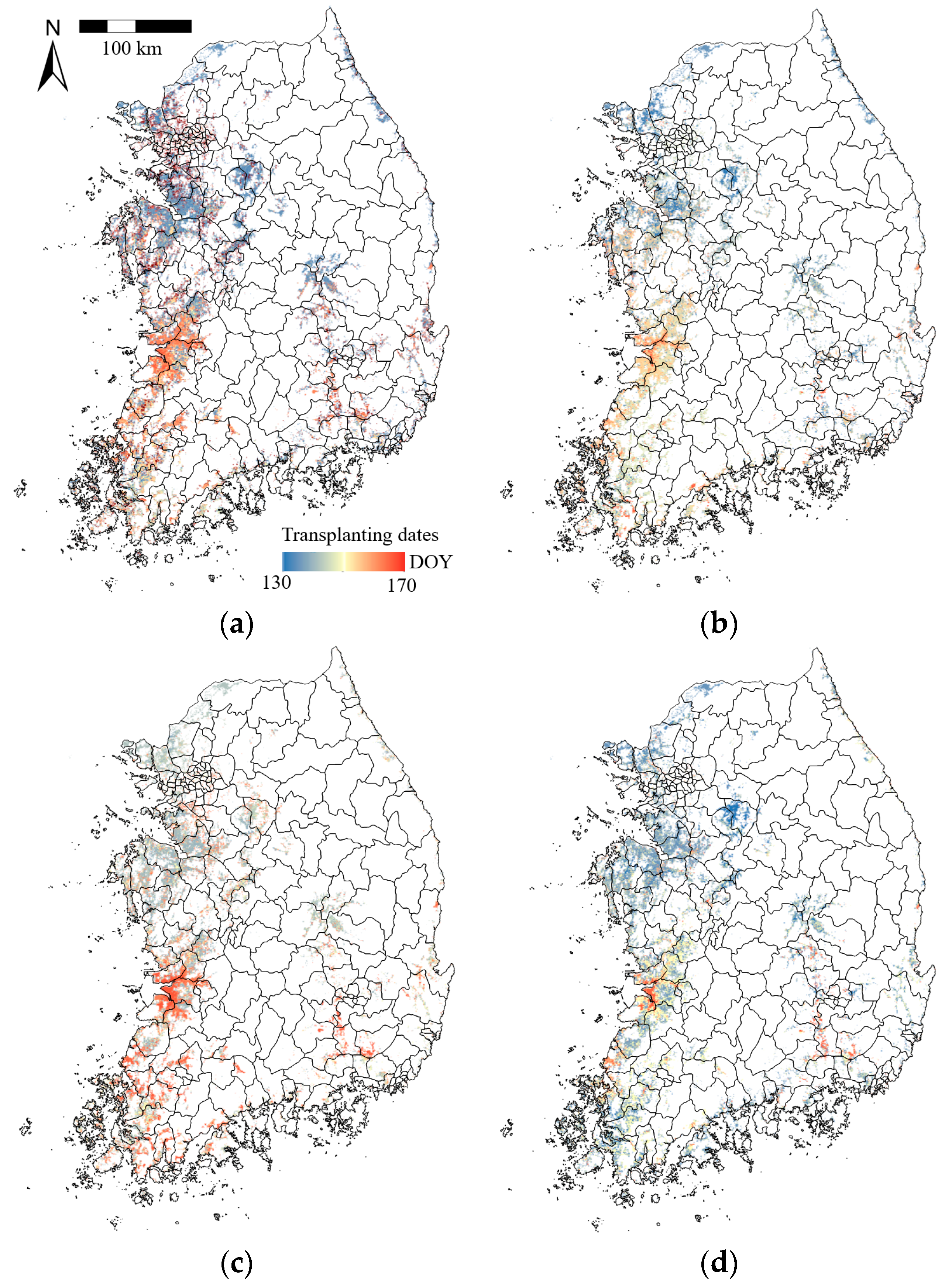
Figure 4.
Detected spatial distributions of transplanting dates (day of year, DOY) for paddy fields derived from Moderate Resolution Imaging Spectroradiometer (MODIS) images in South Korea in (a) 2011, (b) 2012, (c) 2013, and (d) 2014.
Figure 4.
Detected spatial distributions of transplanting dates (day of year, DOY) for paddy fields derived from Moderate Resolution Imaging Spectroradiometer (MODIS) images in South Korea in (a) 2011, (b) 2012, (c) 2013, and (d) 2014.
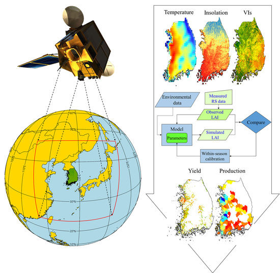
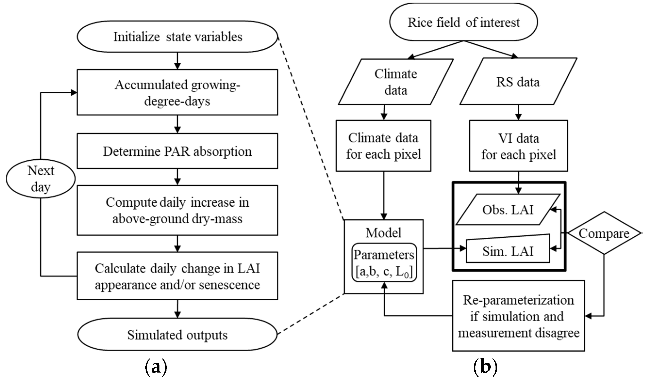
Figure 5.
Schematic diagrams of (a) the daily crop growth simulation process of the GRAMI model and (b) the integrated crop modeling system used to project spatiotemporal crop productions based on the model and remote sensing (RS) data. (LAI: leaf area index, PAR: photosynthetic active radiation, and VI: vegetation index).
Figure 6.
GRAMI model sensitivities: responses of Leaf Area Index, LAI (a) and yield (b) to three parameters to control leaf growth and development, i.e., initial LAI (L0), a, and b.
Figure 6.
GRAMI model sensitivities: responses of Leaf Area Index, LAI (a) and yield (b) to three parameters to control leaf growth and development, i.e., initial LAI (L0), a, and b.
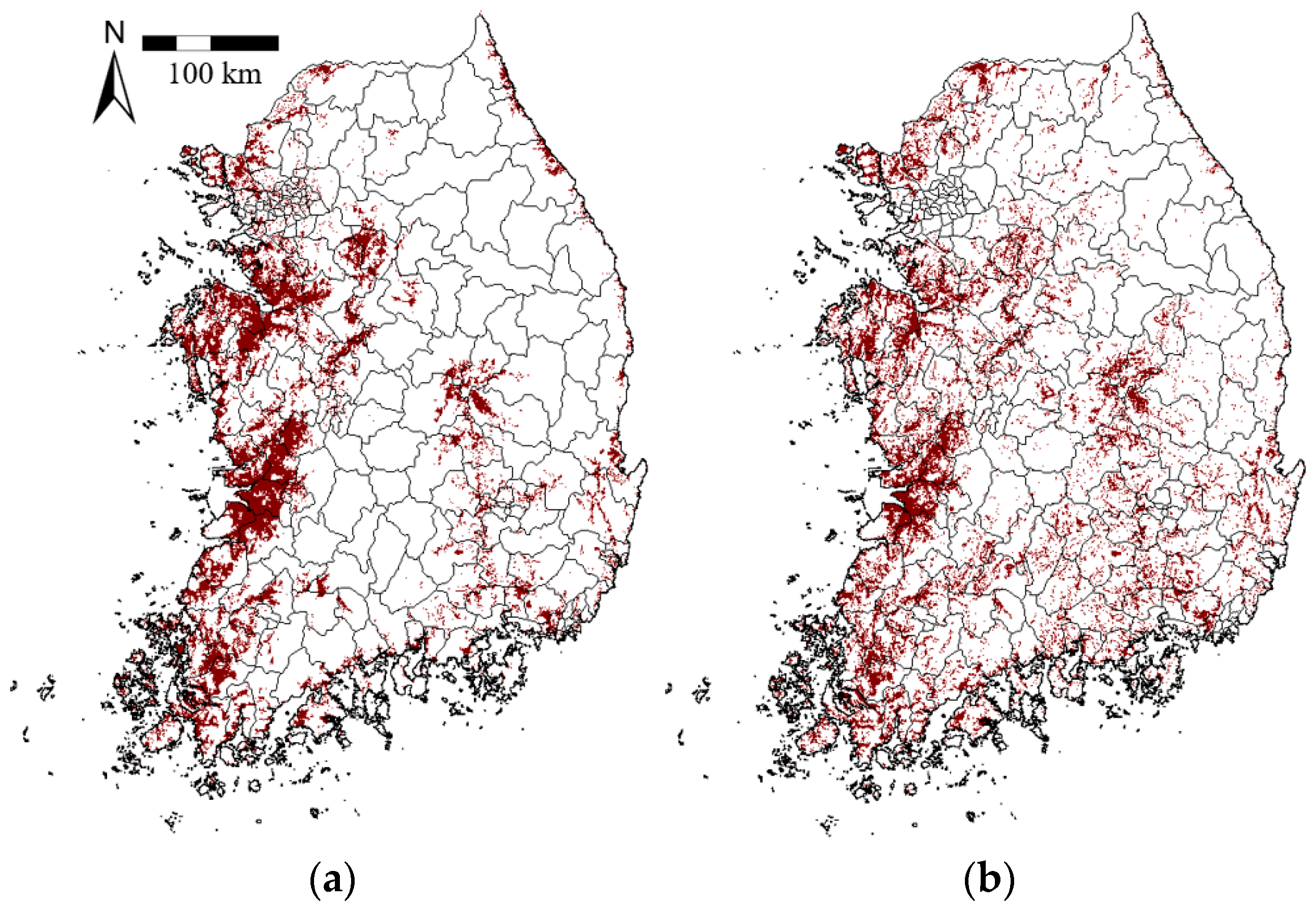
Figure 7.
Comparison of spatial distributions of paddy fields between (a) the Moderate Resolution Imaging Spectroradiometer (MODIS) imagery-based detection map in 2013 and (b) the Korea Ministry of Environment (KME) land cover classification map in South Korea.
Figure 7.
Comparison of spatial distributions of paddy fields between (a) the Moderate Resolution Imaging Spectroradiometer (MODIS) imagery-based detection map in 2013 and (b) the Korea Ministry of Environment (KME) land cover classification map in South Korea.
Figure 8.
Comparisons of estimated paddy areas derived from Moderate Resolution Imaging Spectroradiometer (MODIS) images and the observed paddy areas from the Korean Statistical Information Service (KOSIS) data in South Korea in (a) 2011, (b) 2012, (c) 2013, and (d) 2014.
Figure 8.
Comparisons of estimated paddy areas derived from Moderate Resolution Imaging Spectroradiometer (MODIS) images and the observed paddy areas from the Korean Statistical Information Service (KOSIS) data in South Korea in (a) 2011, (b) 2012, (c) 2013, and (d) 2014.
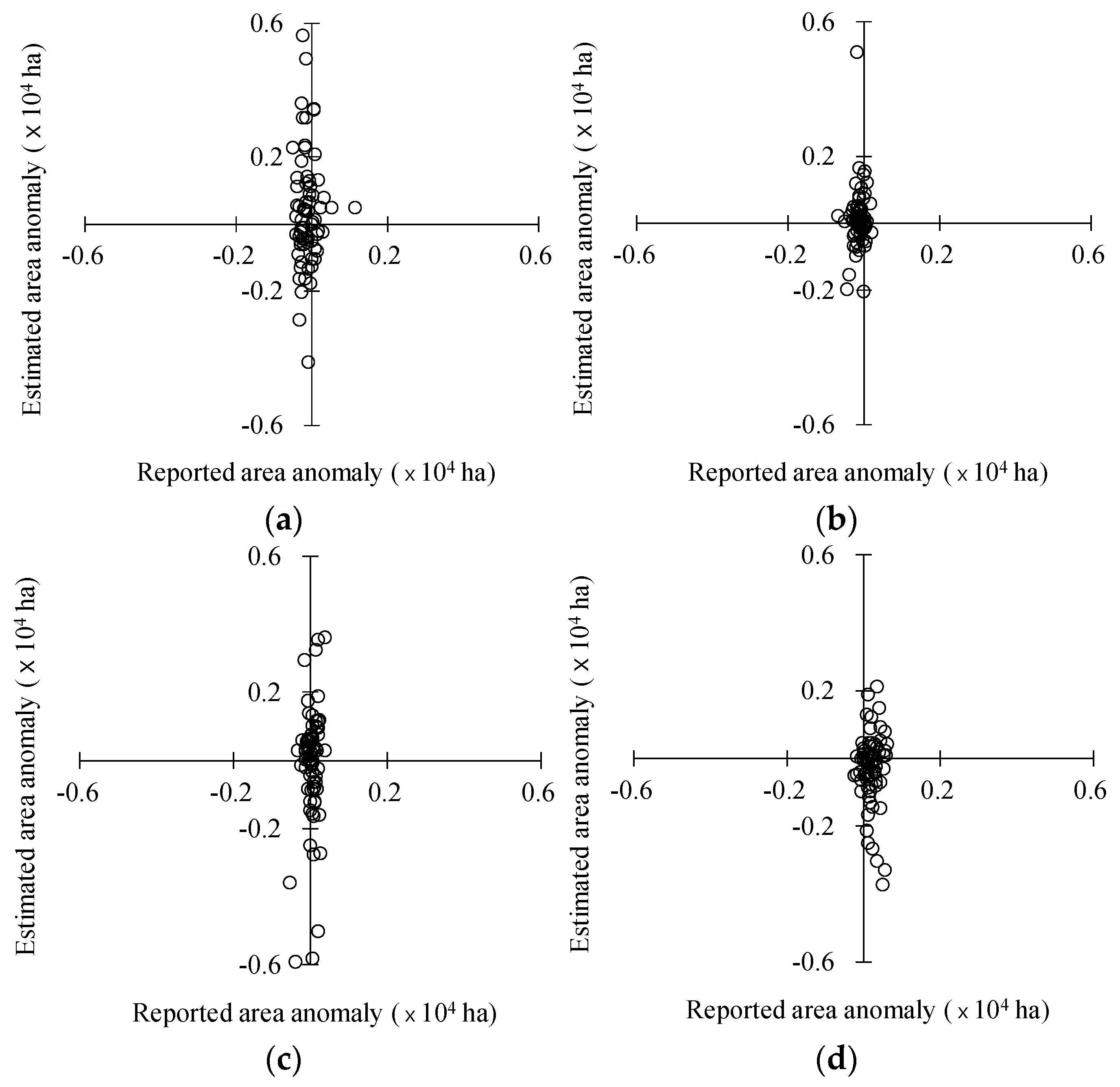
Figure 9.
Anomalies in the paddy areas estimated from Moderate Resolution Imaging Spectroradiometer (MODIS) images and observed from the Korean Statistical Information Service (KOSIS) data in South Korea in (a) 2011, (b) 2012, (c) 2013, and (d) 2014.
Figure 9.
Anomalies in the paddy areas estimated from Moderate Resolution Imaging Spectroradiometer (MODIS) images and observed from the Korean Statistical Information Service (KOSIS) data in South Korea in (a) 2011, (b) 2012, (c) 2013, and (d) 2014.
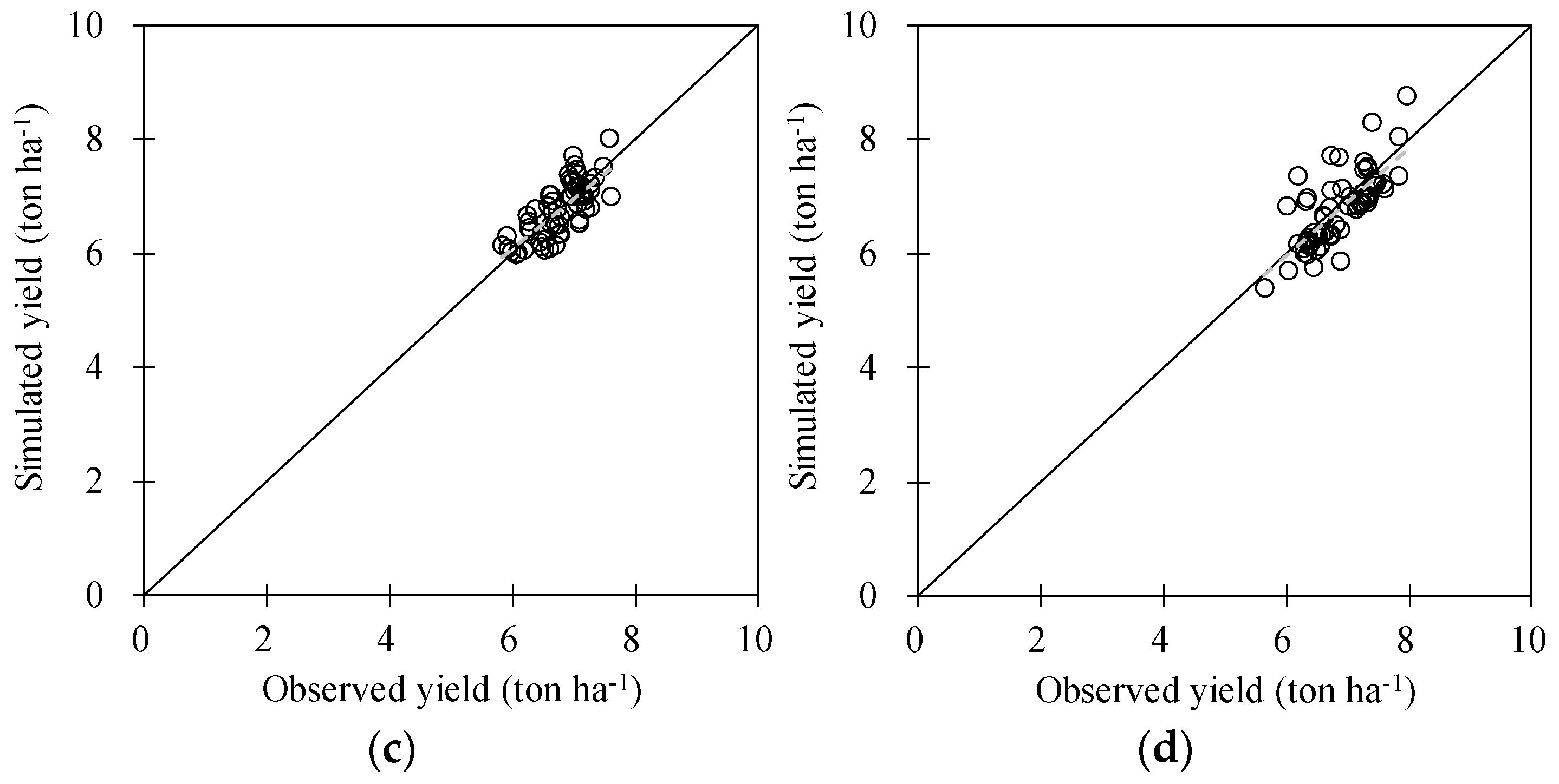
Figure 10.
Comparison of observed and calibrated rice yields in 11 counties of South Korea with more than 5000 ha of the paddy areas from 2011 to 2014. The dashed lines represent linear regression fitting lines between the observed and simulated yields.
Figure 10.
Comparison of observed and calibrated rice yields in 11 counties of South Korea with more than 5000 ha of the paddy areas from 2011 to 2014. The dashed lines represent linear regression fitting lines between the observed and simulated yields.
Figure 11.
Spatial distributions of simulated rice yield using the GRAMI-rice model and geostationary ocean color imager (GOCI) products in South Korea in (a) 2011, (b) 2012, (c) 2013, and (d) 2014.
Figure 11.
Spatial distributions of simulated rice yield using the GRAMI-rice model and geostationary ocean color imager (GOCI) products in South Korea in (a) 2011, (b) 2012, (c) 2013, and (d) 2014.
Figure 12.
Comparison of observed and simulated rice yield in 62 counties of South Korea with more than 5000 ha of the paddy areas from 2011 to 2014. The dashed lines represent linear regression fitting lines between the observed and simulated yields.
Figure 12.
Comparison of observed and simulated rice yield in 62 counties of South Korea with more than 5000 ha of the paddy areas from 2011 to 2014. The dashed lines represent linear regression fitting lines between the observed and simulated yields.
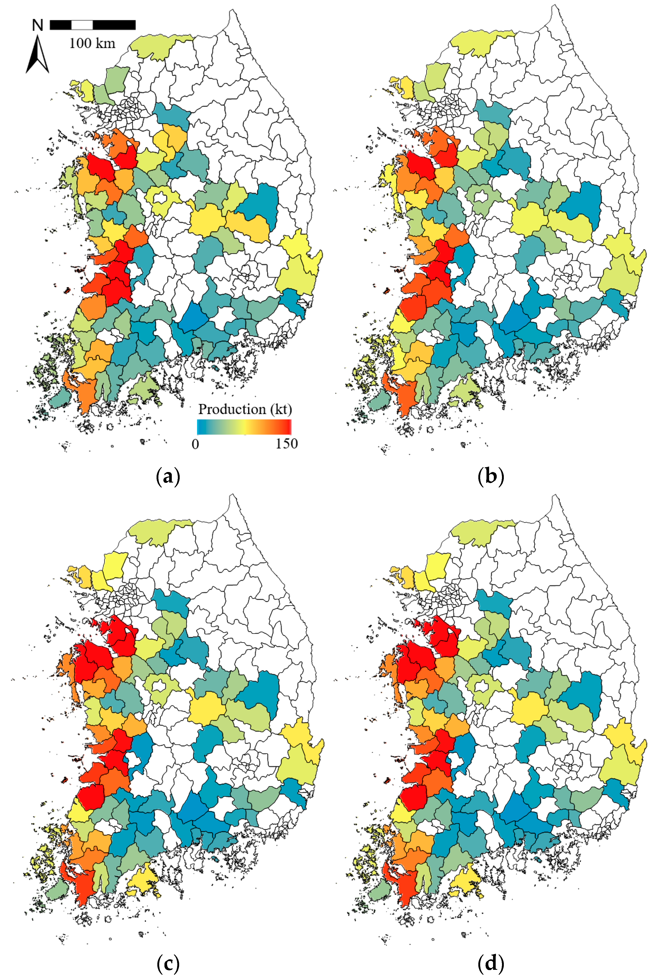
Figure 13.
Spatial distributions of simulated rice production using the GRAMI-rice model and the geostationary ocean color imager (GOCI) products in 73 counties of South Korea with more than 5000 ha of paddy areas in (a) 2011, (b) 2012, (c) 2013, and (d) 2014.
Figure 13.
Spatial distributions of simulated rice production using the GRAMI-rice model and the geostationary ocean color imager (GOCI) products in 73 counties of South Korea with more than 5000 ha of paddy areas in (a) 2011, (b) 2012, (c) 2013, and (d) 2014.
Figure 14.
Comparison of observed and simulated rice production in 73 counties of South Korea with more than 5000 ha of the paddy areas in (a) 2011, (b) 2012, (c) 2013, and (d) 2014.
Figure 14.
Comparison of observed and simulated rice production in 73 counties of South Korea with more than 5000 ha of the paddy areas in (a) 2011, (b) 2012, (c) 2013, and (d) 2014.
Figure 15.
Anomalies in the simulated and observed production in 73 counties of South Korea with more than 5000 ha of the paddy areas in (a) 2011, (b) 2012, (c) 2013, and (d) 2014.
Figure 15.
Anomalies in the simulated and observed production in 73 counties of South Korea with more than 5000 ha of the paddy areas in (a) 2011, (b) 2012, (c) 2013, and (d) 2014.
Table 1.
Collected and manipulated geospatial data information for the detection of the spatial distribution of paddy fields and transplanting dates and for the simulation of rice yield and production in South Korea from 2011 to 2014.
Table 1.
Collected and manipulated geospatial data information for the detection of the spatial distribution of paddy fields and transplanting dates and for the simulation of rice yield and production in South Korea from 2011 to 2014.
| Purpose | Data Type | Produced Data | Spatial Resolution |
|---|
| Detection of paddies and transplanting dates | MODIS land cover | Crop fields | 500 m |
| MODIS reflectance | Vegetation and water indices | 500 m |
| SRTM DEM | Elevation and slope | 90 m |
| KME | Paddy fields | 5 m |
| Simulation of rice yields and production | COMS GOCI | Vegetation indices | 500 m |
| COMS MI | Solar radiation | 1000 m |
| KLAPS | Temperatures | 1500 m |
Table 2.
Information on the wavebands and the spatial resolutions of the Geostationary Ocean Color Imager (GOCI) and Meteorological Imager (MI) sensors aboard the Communication, Ocean, and Meteorological Satellite (COMS).
Table 2.
Information on the wavebands and the spatial resolutions of the Geostationary Ocean Color Imager (GOCI) and Meteorological Imager (MI) sensors aboard the Communication, Ocean, and Meteorological Satellite (COMS).
| COMS Sensor | Wavelength (μm) | Spatial Resolution |
|---|
| GOCI | B1: 0.40–0.42, B2: 0.43–0.45 | 500 m |
| B3: 0.48–0.50, B4: 0.55–0.57 |
| B5: 0.65–0.67, B6: 0.68–0.69 |
| B7: 0.74–0.76, B8: 0.85–0.89 |
| MI | B1: 0.55–0.80 | 1 km |
| B2: 3.50–4.00, B3: 6.50–7.00 | 4 km |
| B4: 10.30–11.30, B5: 11.50–12.50 |
Table 3.
Information on cropland from five land cover classification schemes of the Moderate Resolution Imaging Spectroradiometer (MODIS) MCD12Q1 product.
Table 3.
Information on cropland from five land cover classification schemes of the Moderate Resolution Imaging Spectroradiometer (MODIS) MCD12Q1 product.
| Type Number | Land Classification Scheme | Cropland Class Name from MODIS MCD12Q1 Product |
|---|
| 1 | IGBP global vegetation classification | Cropland | Croplands/natural vegetation mosaic |
| 2 | University of Maryland (UMD) | Cropland | |
| 3 | MODIS-derived LAI/fPAR | Grasses/Cereal crops | Broadleaf crops |
| 4 | MODIS-derived NPP | Broadleaf crops | Annual grass vegetation |
| 5 | Plant Functional type (PFT) | Annual broadleaf vegetation | Broad-leaf crops |
Table 4.
Error statistics of root mean square error (RMSE), Nash–Sutcliffe efficiency (NSE), and paired t-test between observed and estimated paddy areas in 73 counties of South Korea with more than 5000 ha of paddy areas from 2011 to 2014.
Table 4.
Error statistics of root mean square error (RMSE), Nash–Sutcliffe efficiency (NSE), and paired t-test between observed and estimated paddy areas in 73 counties of South Korea with more than 5000 ha of paddy areas from 2011 to 2014.
| Year | Observation | Estimation | RMSE | NSE | t-Test |
|---|
| - | ------------------------- ×104 ha ------------------------- | - | ----- p ----- |
|---|
| 2011 | 0.931 | 0.934 | 0.3982 | 0.154 | 0.980 |
| 2012 | 0.932 | 0.959 | 0.4266 | 0.057 | 0.790 |
| 2013 | 0.917 | 0.982 | 0.4755 | −0.251 | 0.538 |
| 2014 | 0.900 | 1.001 | 0.4592 | −0.198 | 0.331 |
Table 5.
Error statistics of root mean square error (RMSE), Nash-–Sutcliffe efficiency (NSE), and a paired t-test between observed and simulated rice yields in 11 counties of South Korea with more than 5000 ha of paddy areas from 2011 to 2014.
Table 5.
Error statistics of root mean square error (RMSE), Nash-–Sutcliffe efficiency (NSE), and a paired t-test between observed and simulated rice yields in 11 counties of South Korea with more than 5000 ha of paddy areas from 2011 to 2014.
| Year | Observation | Simulation | RMSE | NSE | t-Test |
|---|
| - | -------------------- ton ha−1 ------------------- | - | ----- p ----- |
|---|
| 2011 | 6.64 | 6.71 | 0.284 | 0.627 | 0.732 |
| 2012 | 6.52 | 6.43 | 0.324 | 0.389 | 0.628 |
| 2013 | 6.75 | 6.63 | 0.219 | 0.733 | 0.545 |
| 2014 | 7.00 | 7.11 | 0.306 | 0.622 | 0.692 |
Table 6.
Error statistics of root mean square error (RMSE), Nash–Sutcliffe efficiency (NSE), and paired t-test between observed and simulated rice yields in 62 counties of South Korea with more than 5000 ha of paddy areas from 2011 to 2014.
Table 6.
Error statistics of root mean square error (RMSE), Nash–Sutcliffe efficiency (NSE), and paired t-test between observed and simulated rice yields in 62 counties of South Korea with more than 5000 ha of paddy areas from 2011 to 2014.
| Year | Observation | Simulation | RMSE | NSE | t-Test |
|---|
| - | -------------------- ton ha−1 ------------------- | - | ----- p ----- |
|---|
| 2011 | 6.58 | 6.65 | 0.374 | 0.356 | 0.404 |
| 2012 | 6.36 | 6.26 | 0.451 | 0.468 | 0.296 |
| 2013 | 6.77 | 6.75 | 0.326 | 0.389 | 0.815 |
| 2014 | 6.86 | 6.77 | 0.441 | 0.241 | 0.392 |
Table 7.
Error statistics of root mean square error (RMSE), Nash–Sutcliffe efficiency (NSE), and paired t-test between observed and simulated rice productions in 73 counties of South Korea with more than 5000 ha of paddy areas from 2011 to 2014.
Table 7.
Error statistics of root mean square error (RMSE), Nash–Sutcliffe efficiency (NSE), and paired t-test between observed and simulated rice productions in 73 counties of South Korea with more than 5000 ha of paddy areas from 2011 to 2014.
| Year | Observation | Simulation | RMSE | NSE | t-Test |
|---|
| - | -------------------- kt ------------------- | - | ----- p ----- |
|---|
| 2011 | 61.84 | 62.77 | 27.981 | 0.151 | 0.829 |
| 2012 | 59.37 | 60.10 | 25.227 | 0.167 | 0.908 |
| 2013 | 62.52 | 66.59 | 30.712 | −0.002 | 0.579 |
| 2014 | 62.58 | 69.92 | 33.003 | −0.123 | 0.337 |


