1. Introduction
Human activities and frequent natural disasters accelerate natural land-cover changes on the Earth. Over the past few decades, remote sensing image CD has become the primary solution to effectively monitor changes in large areas. CD is a process that aims at identifying differences in land cover by analyzing the multi-temporal images acquired in the same geographical area [
1]. Timely and accurate CD of natural land cover can provide foundational data for disaster assessment, environmental protection, sustainable development, and maintenance of ecological balance [
2,
3].
The Landsat series of satellites has been providing continuous observation of the Earth’s surface since 1972; its spatio-temporal historical extension is ripe with information that detect land cover changes. Furthermore, the Landsat program has launched seven satellites (Landsat 1, 2, 3, 4, 5, 7, 8) and is equipped with five types of sensors—Multispectral Scanner (MSS), Thematic Mapper (TM), Enhanced Thematic Mapper (ETM+), Operational Land Imager (OLI), and Thermal Infrared Sensor (TIRS)—which have moderate spatial resolution (15–80 m) and short revisit times (16–18 days). These sensors are suitable for observing natural land cover, such as water, soil, coastlines, and vegetation. In addition, since 2008, the US Geological Survey (USGS) has provided more than 11 million current and historical Landsat images free of charge to users over the Internet (
https://earthexplorer.usgs.gov/), with ease of access. Thus, Landsat imagery has been widely used in monitoring the natural land cover changes caused by floods [
4], forest fires [
5,
6], and glacial melting [
7].
Interferences in Landsat images include Gaussian noise and local brightness distortion; it is not sensitive to the changes of small objects. On one hand, the process of acquiring a remote sensing image—from acquisition to transmission—is inevitably affected by different degrees of noise, e.g., speckle noise in SAR images and Gaussian noise in optical satellite images. On the other hand, Landsat satellites carry passive sensors that record electromagnetic energy; however, the passive sensors are sensitive to the difference in illumination and atmospheric conditions. Therefore, the multi-temporal Landsat images generally have a difference in local brightness [
8]. In addition, since intra-class variation and inter-class variation in the Landsat image are relatively small, the expression of changed details is weak.
As the spatial resolution of the Landsat image is not high (≥15 m) and the intra-class variability in the image is small, pixel-based methods are suitable for Landsat image CD, which can be further divided into threshold-based or classification-based [
3]. In the threshold-based method [
9,
10,
11,
12,
13], it is crucial to analyze the statistical distribution of DI and find the optimal threshold to distinguish changed pixels from the unchanged ones. For example, Kittler and Illingworth proposed a minimum-error thresholding algorithm (KI), which determines the threshold by optimizing the average pixel classification error rate [
11]. The expectation maximization (EM) algorithm automatically selects the decision threshold by minimizing the overall CD error probability under the assumption that pixels in the DI are independent [
9]. Zanetti constructed a compound model to describe the statistical distribution of the DI, and the threshold value was determined by the EM algorithm and Bayes decision [
12]. Threshold-based methods are efficient and useful. However, they require an accurate estimation of the DI statistical distribution and decision threshold, and are sensitive to image interferences. The Markov random field (MRF) model was introduced to integrate the spatial-contextual information included in the neighborhood of each pixel, and it can remove small false detection regions [
9]. However, MRF also requires the selection or estimation of a model for the statistical distribution of the changed and unchanged classes.
As CD is essentially a classification problem, there exist in literature both supervised and unsupervised approaches (clustering-based) to address it [
14,
15,
16,
17,
18,
19,
20,
21]. A set of training data is required for the supervised methods, while there is no need for training data in the clustering-based methods. Thus, the clustering-based methods are commonly applied in real applications. Clustering is a classification process under the assumption that samples of the same cluster are more similar to one another than samples belonging to different clusters. In clustering-based CD methods, because the image pixels belonging to different clusters cannot be separated with sharp boundaries, one of the most popular methods is the fuzzy c-means (FCM) algorithm [
17,
18,
19,
20,
21]. The conventional FCM algorithm is not robust to image noise and local brightness distortion because the spatial-contextual information is not taken into account [
17]. Krindis and Chatzis proposed a fuzzy local information c-means clustering algorithm (FLICM), which uses a fuzzy local similarity measure to resist image noise. In particular, a fuzzy factor is introduced into its objective function to enhance the clustering performance [
18]. Gong et al. proposed a reformulated fuzzy local-information c-means clustering algorithm to classify the changed and unchanged regions in the fused DI [
19]. However, fuzzy clustering-based CD methods are sensitive to the initialization of the clusters and easily get stuck to the local minima because the distribution of DI is complex due to image interferences.
Since EAs have promising optimization ability, which can jump out of the local minima, EAs-based optimal clustering has been applied to band selection [
22], image classification [
23,
24,
25], and change detection [
8,
20,
21,
26,
27,
28,
29,
30,
31,
32]. Celik used the genetic algorithm (GA) to generate optimal CM with minimum mean square error (MSE) [
20]. This method is suitable for CD on different types of satellite images. However, the algorithm is sensitive to image interferences and converges slowly due to its encoding strategy, which is based on the whole binary mask. Ghosh et al. proposed a context-sensitive CD method, which adopts a mean filter to remove the image noise in DI and uses GA to evolved the changed and unchanged clusters [
21]. Li et al. proposed an evolutionary multi-objective fuzzy clustering method, which can obtain a set of clusters with different trade-offs between removing noise and preserving detail [
28]. However, filtering will blur the weak changed details, especially on boundaries or edges, and it cannot resist local brightness distortion in the multi-temporal images. Thus, although the above EAs-based methods can obtain optimal clusters, they are overly dependent on the DI and are affected by image interferences, resulting in inaccurate detection results.
In order to reduce image interferences and improve CD accuracy, we propose an unsupervised CD method based on multi-feature clustering using DE algorithm (M-DECD) for Landsat Imagery. In M-DECD, according to characteristics of Landsat images, the Wiener filter, edge detection and structural similarity (SSIM) index are used to extract spectral-spatial features from the multi-temporal images and DI. To obtain optimal clusters in the multi-feature space, a CD method based on DE algorithm and FCM is proposed and an adaptive strategy adopted to adjust DE’s control parameters. Compared to previous works, the major contributions of this paper are as follows.
- (1)
The optimal multi-feature clustering-based CD framework. This framework is composed of two steps. In the first step, a suitable multi-feature space is constructed according to characteristics of the data. In the second step, an EA is adopted to search for optimal CD clusters using the minimum clustering index. The binary CM can be generated according to the distance between the pixels and the clusters.
- (2)
A multi-feature space for Landsat images CD. Three complementary spectral-spatial features are extracted from the multi-temporal images and DI, including the Wiener de-noising, structural similarity, and detail enhancement, which are designed to resist the interference of the Gaussian noise and local brightness distortion, while preserving weak changes.
- (3)
Adaptive DE algorithm for the optimization of CD results. Since the DE algorithm has promising global optimization capabilities, it is employed to search for the optimal changed and unchanged clusters in the complex multi-feature space. The two clusters are encoded into an individual, and the objective function derived from the FCM is utilized to evaluate the quality of clusters. The genetic operators, i.e., crossover, mutation and selection are used for evolutionary processes. In addition, the control parameters of DE, i.e., the scaling factor F and crossover rate CR, which have significant influence on optimization performance, have been adaptively adjusted to improve the robustness of the proposed method.
The experimental results show that the M-DECD is robust to interferences of Landsat images, and it can preserve some weak changed edges of small objects. Compared with the conventional methods and the state-of-the-art methods based on evolutionary clustering, M-DECD can generate a better CM and improve detection accuracy, especially in the Canada dataset.
This paper is organized as follows.
Section 2 briefly introduces the FCM algorithm and the basic DE algorithm.
Section 3 presents the methodology of the proposed M-DECD, including the construction of multi-feature space and the adaptive DE algorithm. Dataset description, experimental results, and parameters analyses are presented in
Section 4. Finally, the conclusions are drawn in
Section 5.
3. Proposed Methodology
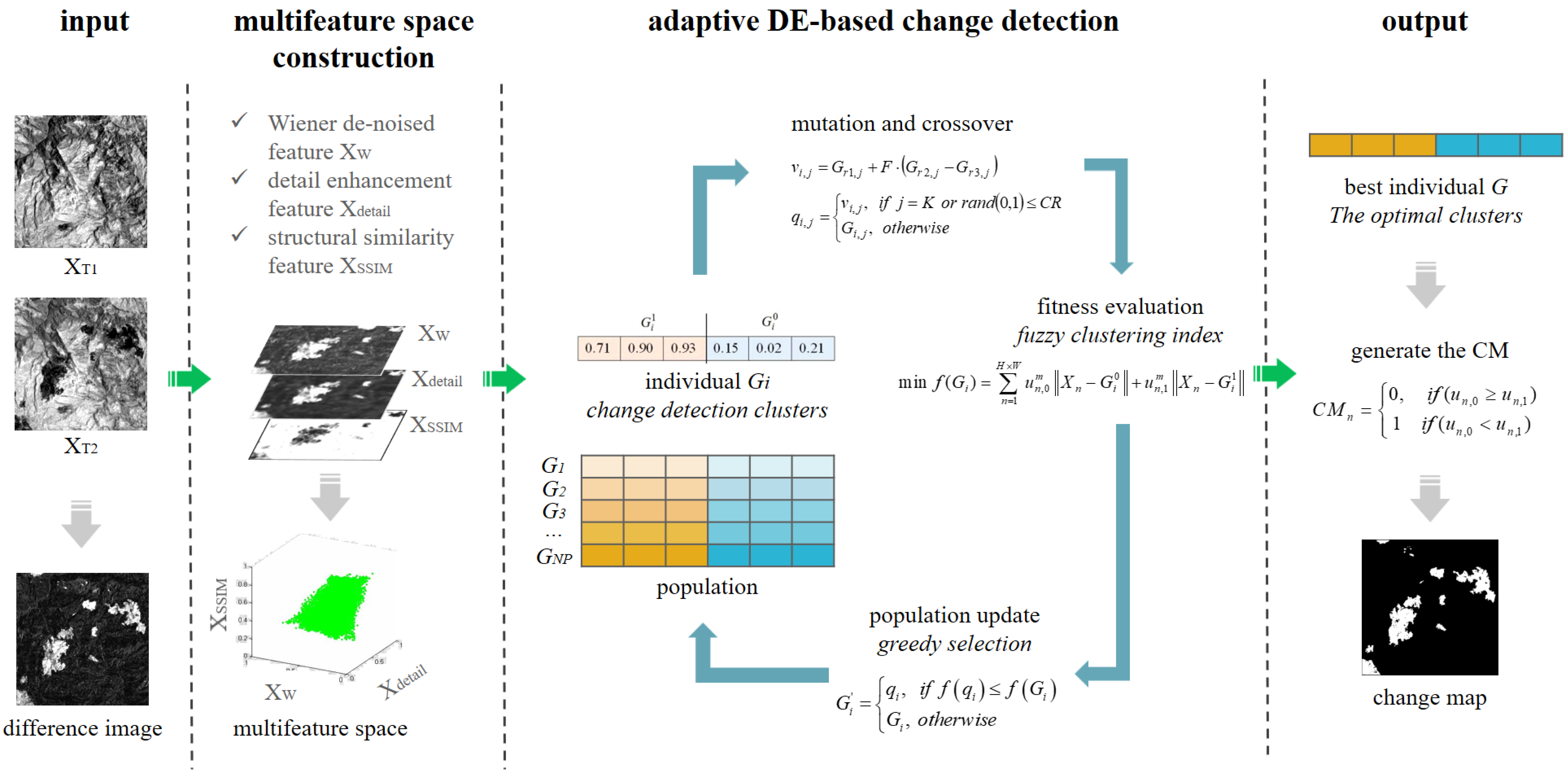
The framework of the proposed M-DECD (shown in
Figure 1) is composed of two main steps: (1) Constructing a multi-feature space from the multi-temporal images and DI; and (2) adopting the adaptive DE algorithm to search for the optimal changed and unchanged clusters and generate the binary CM. For a better understanding, the meaning of commonly used symbols is listed in
Table 3.
We assume that two co-registered images and of size are captured over the same geographical area at two different times, and , respectively. The purpose of the M-DECD is to generate an accurate CM, , where .
The first step of the M-DECD is to calculate a DI using multi-temporal images
and
. For the Landsat images, we use the images subtraction to compute the DI (
), which calculates the absolute value of the spectral difference.
3.1. Multifeature Space Construction
According to the characteristics of Landsat images, a multi-feature space is constructed to resist the interferences of Gaussian noise and local brightness distortion, while preserving important weak changes. The multi-feature space consists of three complementary elements: Wiener de-noising, the detail enhancement and structural similarity, which are extracted from multi-temporal images and DI.
3.1.1. Wiener De-Noised Feature
Image denoising is an important step in digital image processing, and it can effectively reduce the small false detection regions in CD. The evolutionary clustering-based CD methods apply mean filtering to the difference image and utilize the average value of the neighborhood pixels as the spatial feature [
21,
28]. Although the mean filter can remove some image noise, it will blur important changed details, such as boundaries or edges.
For Landsat images, Gaussian noise is generated by the resistive components of the receiver. Since the Wiener filter can effectively remove Gaussian noise and retain the high-frequency information of the image (e.g., boundaries and edges), in M-DECD, we apply Wiener filtering to the DI and generate the Wiener de-noised feature. The Wiener filter removes the noise by minimizing the MSE between the output image and the expected result, and it can adaptively conduct smoothing according to the local image variance. When the local variance is large, it performs little smoothing, and vice versa. Therefore, the quality of filtering result will not decrease drastically with an increase of the filter window size [
36].
The Wiener filter [
37] estimates the local mean
and variance
around each pixel using Equations (6) and (7), respectively. The Wiener de-noised feature
is then calculated using Equation (8).
is the
local neighborhood of each pixel in
, and
is the average of the local estimated variances.
3.1.2. Detail Enhancement Feature
For Landsat images, the intra-class variation and inter-class variation are relatively small, and the expression of changed details is weak, especially at the edge of the changed region. Thus, except for the noise removal, another challenge of Landsat images CD is detail preservation. In [
38], a modified Perona-Malik filter was employed to remove image noise and extract stable edges for CD. In [
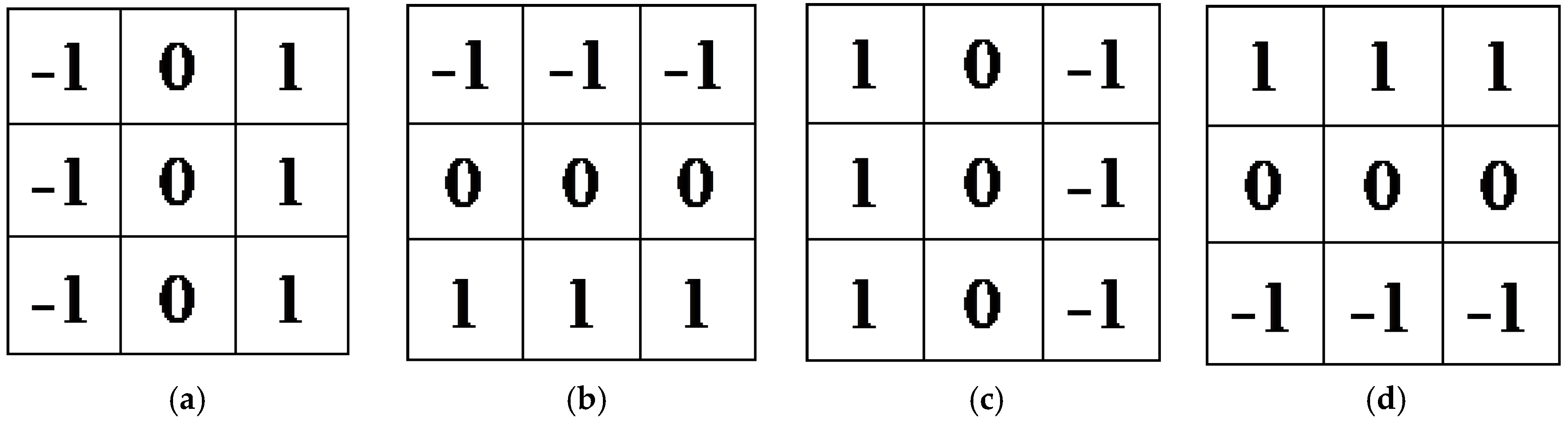
39], a novel edge-preserving MRF method for CD was proposed, which integrated the edge and detail-preserving information in the MRF modeling. In the proposed M-DECD, the image details are enhanced by fusing the edge features with the DI. In order to obtain a full range of edge features, four edge detection operators of different directions are applied to the DI, including 0°, 90°, 180°, and 270°. The convolution templates are shown in
Figure 2.
After extraction of multiple edge features
, in order to prevent abnormal sample data possibly arising out of the multiple features from interfering with the subsequent change judgment, all the features need be normalized to [0, 1]. The DI is then combined with the edge features using the weighted sum strategy and the detail enhancement feature
is defined as:
3.1.3. Structural Similarity Feature
In order to resist the local brightness difference between the multi-temporal Landsat images, the SSIM [
40] was utilized to measure the similarity between the multi-temporal images, and is calculated based on local luminance, contrast, and structure comparisons. The SSIM has been used in various applications, such as image compression [
40], video surveillance, and object detection [
41]. In [
8], the difference image was obtained by the SSIM.
The SSIM uses three components, including luminance
, contrast
, and structure
, to compute the structural similarity feature
using Equation (10), where
,
, and
are the exponents used to adjust the influence of each measurement. In M-DECD,
. The variables
,
, and
are calculated using Equation (11).
where
,
, and
are the mean, standard deviation, and cross correlation between
and
, respectively.
,
, and
are small positive constants to avoid instability. The image statistics (
,
, and
) are computed as proposed in [
40].
If is close to 1, it indicates that the local structures of the two-phase images have a high similarity. On the contrary, if is close to 0, it means that the local structures of the two-phase images are quite different.
After extracting the Wiener de-noised feature, the detail enhancement feature and the structural similarity feature, a multi-feature space is constructed by stacking these feature maps. Then, each pixel in the DI can be mapped to a data point in the multi-feature space and the CD is transformed to a classification problem, and it is crucial to find the optimal changed and unchanged clusters in the multi-feature space.
3.2. Adaptive Differential Evolution-Based Change Detection
In M-DECD, a CD method based on adaptive DE algorithm and FCM is proposed. The DE is employed to search the optimal clusters in the multi-feature space by minimizing the objective function derived from FCM. Input the multi-feature data , then randomly generate a set of potential clusters in the multi-feature space, and produce new clusters through mutation and crossover of DE algorithm. The Jm distance of FCM is used as the objective function of DE to evaluate the quality of these clusters, and those elite clusters with smaller objective function value will survive to the next generation until the process reaches the maximum iterations. Finally, output the optimal clusters and the multi-feature data can be divided into changed and unchanged classes according to their fuzzy membership to the optimal clusters. The adaptive DE-based CD method is composed of four steps, which are described as follows:
3.2.1. Population Initialization
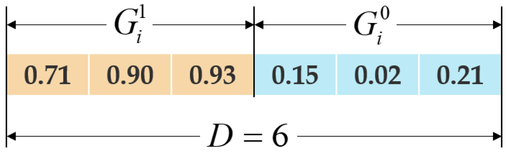
The population consists of
NP individuals,
. Each individual represents a candidate solution of the CD problem, i.e., a vector of changed and unchanged clusters, as shown in
Figure 3. Each individual in the population is randomly generated in the multi-feature space.
where
,
,
represents the
j-th dimension of the
i-th individual in the population, and
is the dimension of the two clusters.
and
correspond to the minimum and maximum values in the
j-th dimension of the input multi-feature data, respectively, and
is a random value between
and
.
3.2.2. Fitness Evaluation
The objective function is modeled according to the fuzzy clustering-based CD problem. In this paper, we adopted the
Jm distance of FCM, which is designed to minimize the intra-class distance, as the objective function of DE algorithm. Fitness is the objective function value of each individual, which can evaluate the quality of the solution. The purpose of DE is to obtain CD clusters with the minimum fitness value. The fitness of individual
can be calculated using Equation (13).
where
is a
-dimension individual consisting of changed cluster
and unchanged cluster
.
is a
-dimension vector which denotes the
n-th point of the multi-feature data
.
is the fuzzy membership which represents the probability of belonging of point
to the cluster
, and it is calculated according to Equation (2).
represents the intraclass distance of unchanged pixels, and
represents the intra-class distance of changed pixels.
3.2.3. Mutation and Crossover
DE upsets the current population with the scaled difference of randomly selected and distinct individuals. For each target individual
, we randomly pick three exclusive individuals
from the current population and generate a mutant individual
using Equation (14). The mutant individual is a vector of potential clusters around the target individual.
is the scaling factor.
has to be constrained according to the domain of multi-feature space.
In order to produce a desirable vector of clusters, the crossover operator is then applied to the mutant individual
to generate a trial individual
using Equation (15), where
is the crossover rate.
is a random integer between 0 and
D.
Two control parameters (scaling factor
F, crossover rate
CR) affect the optimization result. If properly designed, an adaptive strategy can enhance the robustness of the algorithm and improve the convergence rate. In the M-DECD, a self-adaptive strategy is adopted, and it can dynamically adjust the parameters according to the fitness of the individual (details can be found in [
42]). The mutation rate
is adaptively determined by Equation (16), which means that a vector of clusters with a smaller fitness is more likely to retain its control parameters. Before performing mutation and crossover, the new control parameters
and
are updated using Equations (17) and (18), respectively.
where
denotes the uniform random values within the range [0,1],
is the iteration number,
is the maximum iterations. In the initial generations, adaptive DE tends to search the solutions in the multi-feature space uniformly and, in the later generations, it tends to search the solutions near the optimal clusters.
3.2.4. Selection
To keep the population size a constant, DE applies the greedy selection strategy to decide whether the new solutions can survive to the next generation or not, which is executed between the target individual
and trial individual
using Equation (19), where
is the
i-th individual in the next generation, and
is the objective function.
After selection, potential clusters with smaller Jm distance are preserved. The evolutionary process should be repeated until the number of iterations reach the maximum, Finally, output the optimal clusters and its fuzzy membership .
3.2.5. Generation of the Change Map
The optimal CM can be obtained by assigning a label (0: unchanged, 1: changed) to each pixel according to its fuzzy membership.
3.3. Computational Complexity of the M-DECD Algorithm
The computational complexity of M-DECD can be split into two parts: (1) the construction of the multi-feature space; (2) the adaptive DE clustering-based CD. We assume that the size of the input image is M×N, and the dimension of the multi-feature space is D, then the computational complexity for part (1) is O(M×N×D). The adaptive DE clustering-based CD can be further split into six steps as follows:
- (1)
Population initialization. The computational complexity should be O(L × NP), where L denotes the length of the individual, i.e., dimension of the changed and unchanged clusters.
- (2)
Fitness evaluation. The fitness of each individual is calculated based on the input data, so the computational complexity of the fitness evaluation of NP individuals should be O(M × N × NP).
- (3)
Population optimization. This step is composed of fitness evaluation, mutation, crossover and selection. The whole computational complexity should be O(L × NP × G), where G is the maximum generations.
- (4)
Generation of the change map. The computational complexity should be O(M × N).
4. Experiments and Analysis
In order to demonstrate the effectiveness of the M-DECD, four real Landsat datasets were tested in the experiments. Seven pixel-based methods for remote sensing images with moderate spatial resolution are presented, including a threshold-based method (KI [
11]), a spatial-contextual method (Markov random field expectation maximization, MRF+EM [
9]), fuzzy clustering-based methods (FCM [
17]; fuzzy local information c-means algorithm, FLICM [
18]), and EA-based methods (genetic algorithm encoding change mask, GA-mask [
20]; genetic algorithm combined with FCM algorithm, GA-FCM [
21]; multi-objective EA with spatial information, MOEA/D [
28]).
The CD result is a binary CM, where the white pixels in the map represent the changed objects, and the black pixels represent the unchanged objects. In order to quantitatively analyze the experiment results, we compare the CMs with the reference image. Generally speaking, the false alarms (FAs), missed alarm (MAs), overall error (OE), and kappa coefficient are commonly used as evaluation indexes to assess the result of CD. MA represents the number of pixels that are classified into the unchanged class but are changed in the reference image. FA denotes the number of pixels, which are classified into the changed class but are unchanged in the reference image. OE is defined as:
The kappa coefficient is usually applied to evaluate the effect of the classification. A higher value of kappa indicates a better detection result. Kappa can be calculated as:
where
PCC represents the percentage of correct classification,
PRE represents the proportion of expected agreement.
PCC and
PRE are defined by Equations (23) and (24).
where
is the number of image pixels.
is the number of changed pixels that are correctly classified, and
is the number of unchanged pixels that are correctly classified.
and
are the number of changed pixels and unchanged pixels in the reference image, respectively.
4.1. Dataset Description
4.1.1. Mexico
The Mexico dataset is an open-access dataset for change detection evaluation. It is made up of two images acquired by the ETM+ sensor of the Landsat-7 satellite in an area of Mexico on 18 April 2000 and 20 May 2002. The spatial resolution was 30 m. A section of 512 × 512 pixels was selected as the test site. Between the two acquisition dates, forest fires destroyed a large proportion of the vegetation. Band 4 (spectral range from 0.775 μm to 0.900 μm) was selected in our experiment, because band 4 of the ETM+ sensor is the near-infrared band, which is sensitive to the difference of vegetation type.
Figure 4a,b shows the band 4 of the images 2000 and 2002, respectively. The reference map was manually defined according to a detailed visual analysis of the available multi-temporal images and the difference image. The reference map contained 25,599 changed pixels and 236,545 unchanged pixels. No radiometric correction was applied.
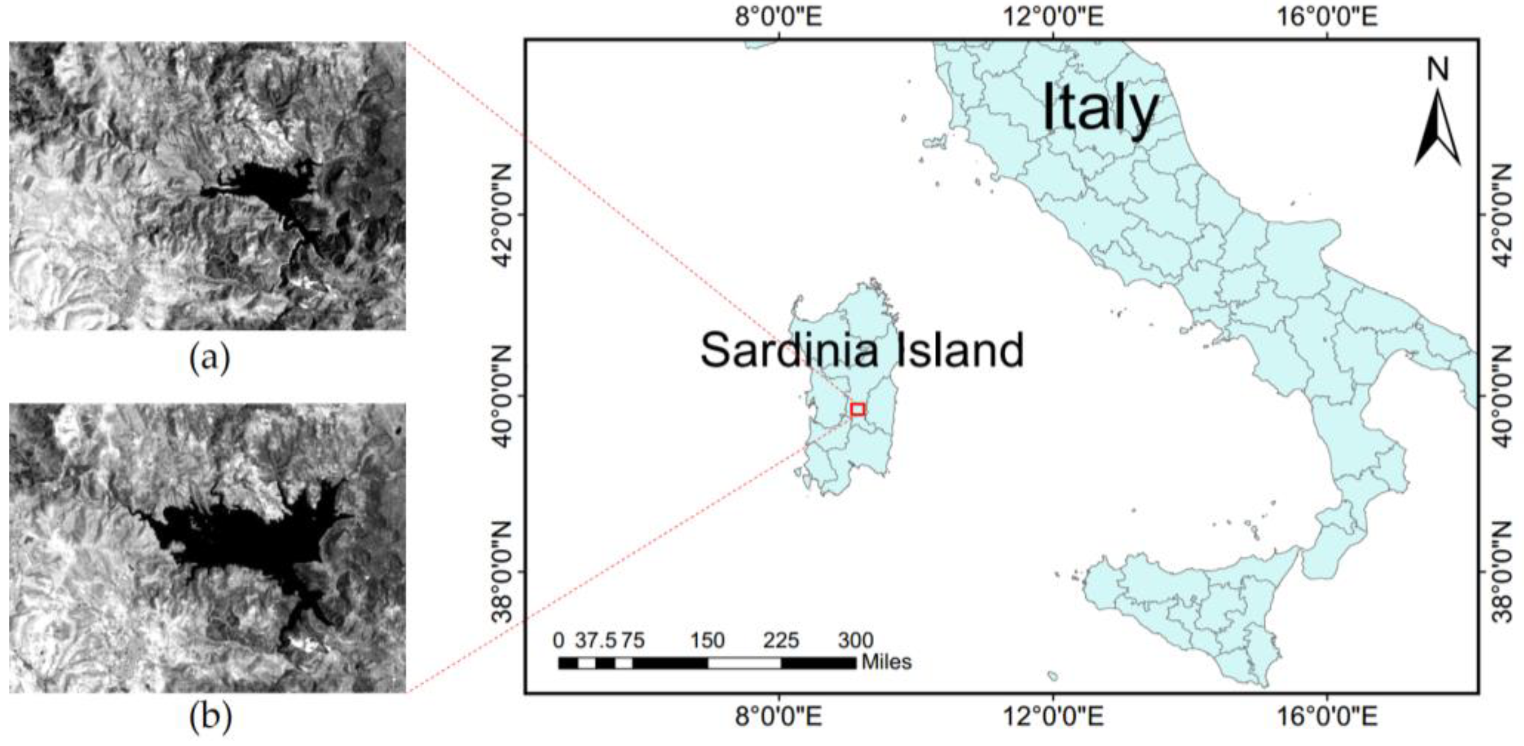
4.1.2. Sardinia Island
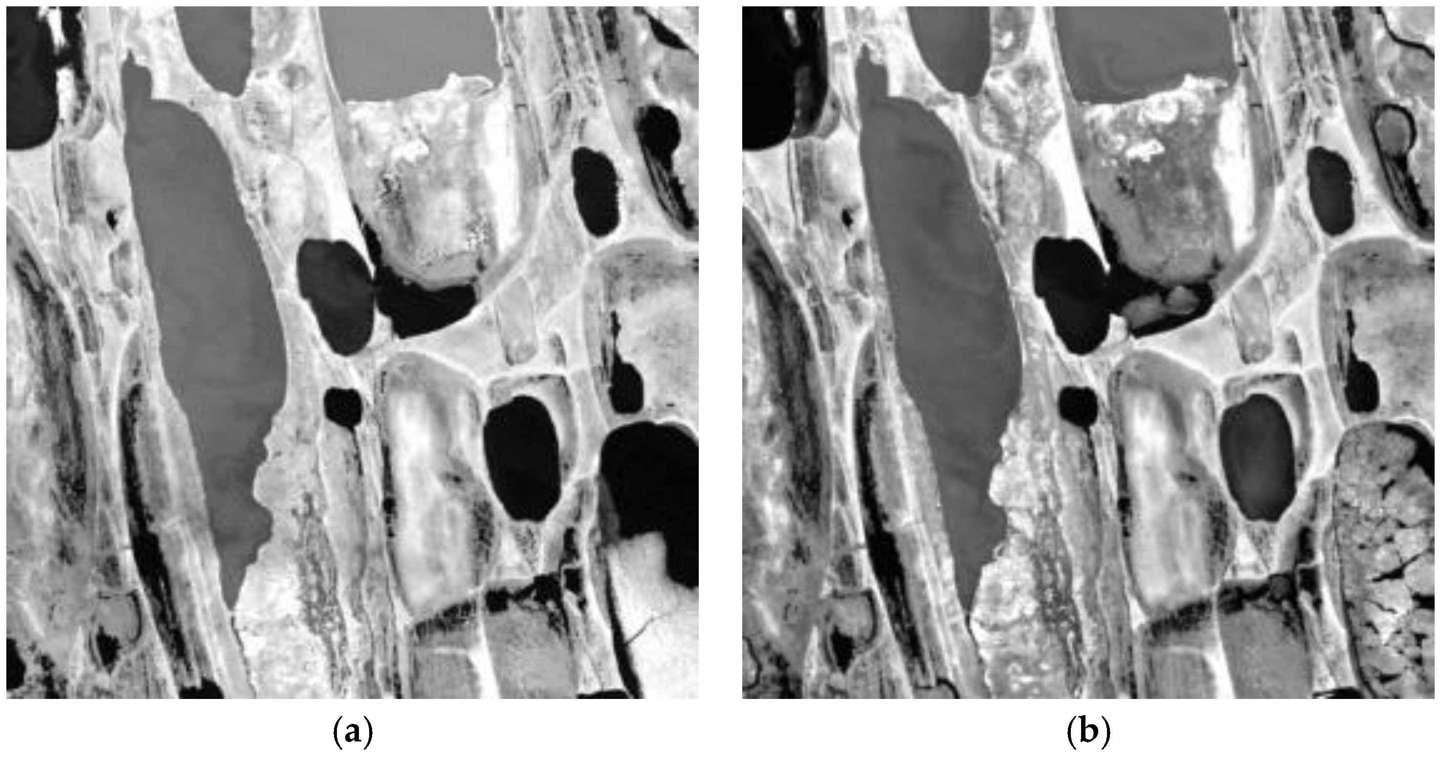
The second dataset tested in our experiment is the Sardinia island dataset, which is composed of two multispectral images acquired by the TM sensor of the Landsat-5 satellite in September 1995 and July 1996. The spatial resolution was 30 m. The test site was a section of 300 × 412 pixels of a scene covered Lake Mulargia on the island of Sardinia. Between the two acquisition dates, the water level of the lake increased due to the flood. Band 4 (spectral range from 0.760 μm to 0.960 μm) of the TM sensor is the near-infrared band, because water has a strong absorption effect in the near-infrared band, which makes the water profile clear in band 4.
Figure 5a,b show the tested image 1995 and image 1996, respectively. The reference map was manually defined, in which 7480 changed pixels and 116,120 unchanged pixels were identified. No radiometric correction was applied to the multi-temporal images. The images were co-registered with 12 ground control points.
4.1.3. Alaska
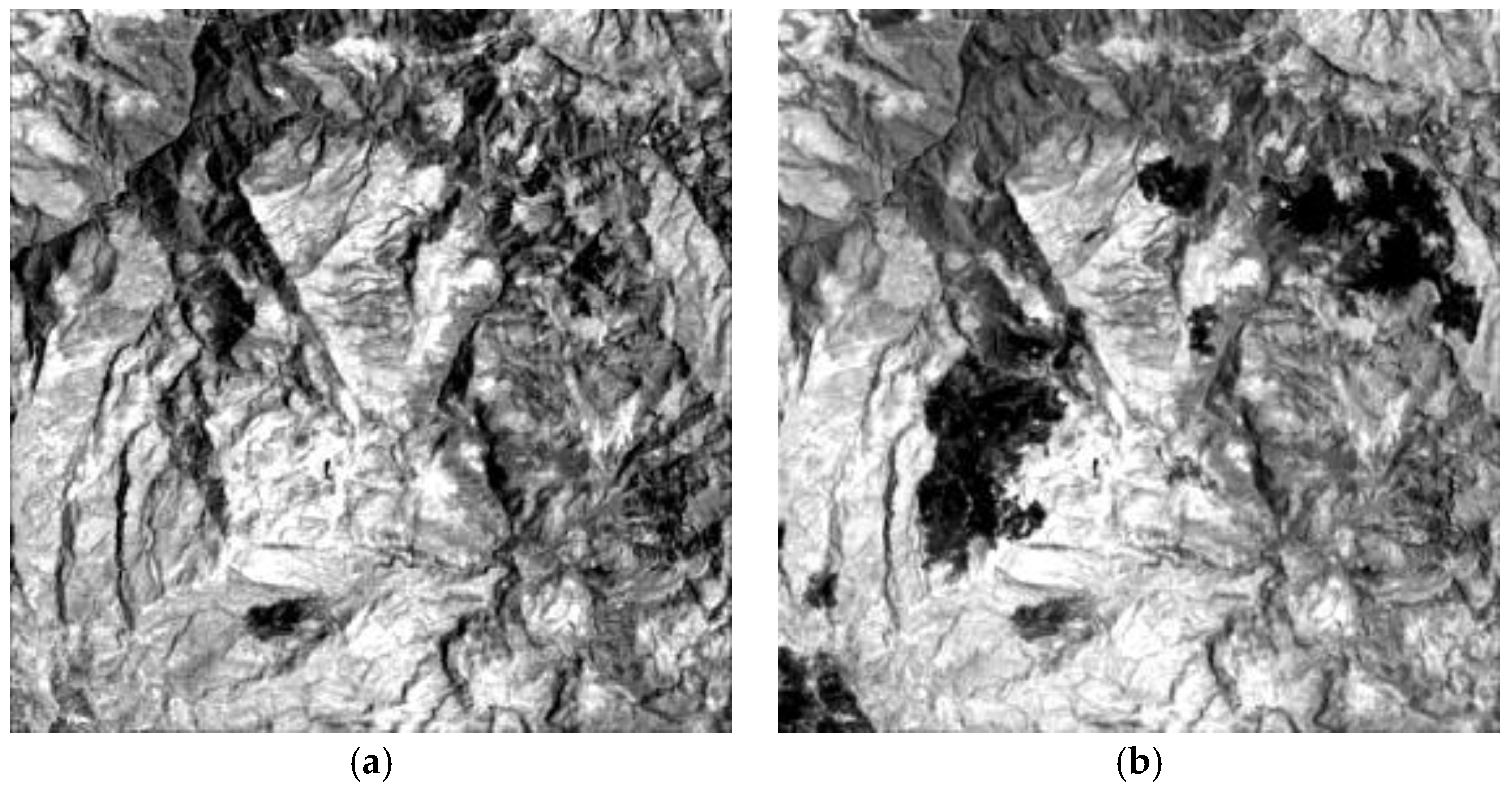
The third dataset is the Alaska dataset, which is made up of two multispectral images acquired by the TM sensor of the Landsat-5 satellite in July 1985 and July 2005. The spatial resolution was 30 m. Band 4 was selected for the experiment for the same reasons mentioned above. A section of 400 × 400 pixels was selected for the experiment.
Figure 6a,b display the tested images. The reference map contains 9741 changed pixels and 150,259 unchanged pixels. No radiometric correction was applied to the multi-temporal images. The former image was registered to the latter one.
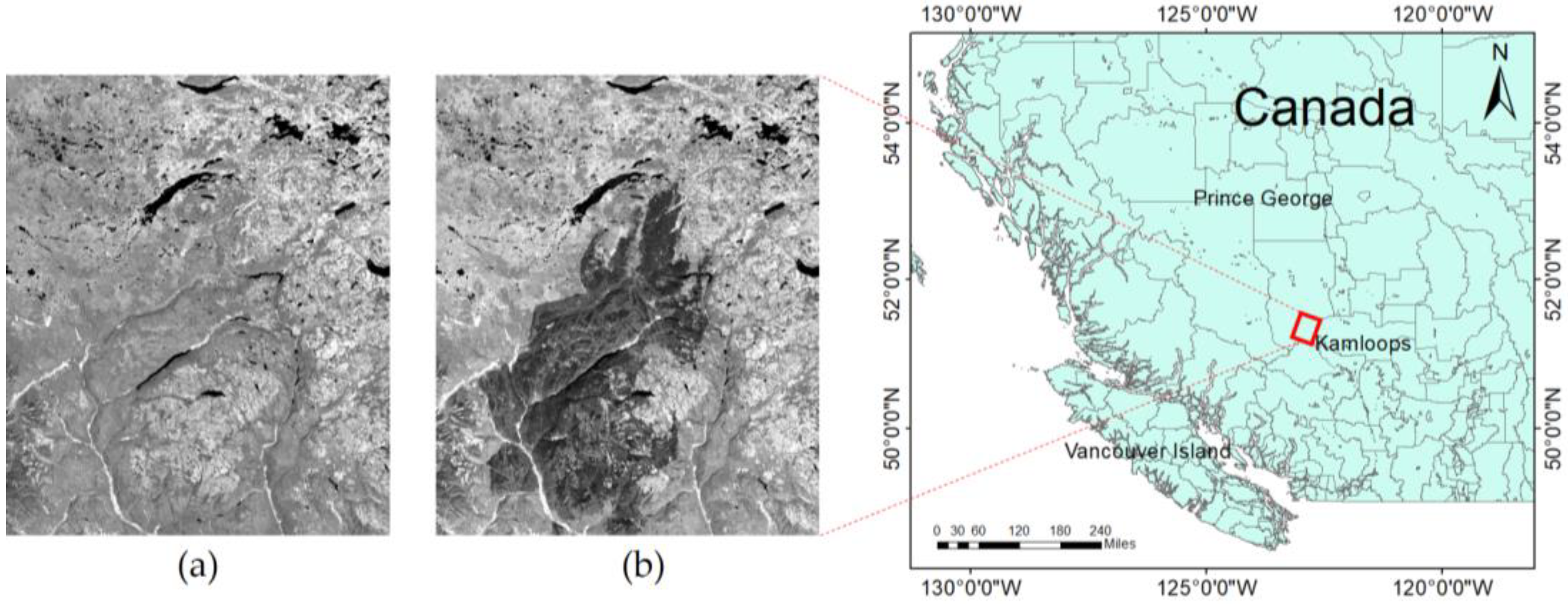
4.1.4. Canada
The Canada dataset is composed of two multispectral images acquired by the Landsat-8 OLI sensor on 2 July 2017 and 22 August 2017. The spatial resolution was 30 m. The test site is a scene near Prince George, British Columbia, Canada. The size is 3000 × 2500 pixels, which is much bigger than the above three datasets. The forest fires lasted more than two weeks, which led to the suspension of three major timber producers, and more than 14,000 people had to be evacuated. In order to accurately detect the disaster area in the forest, we selected band 5 for our experiments. Band 5 (spectral range from 0.845 μm to 0.885 μm) belongs to the near-infrared band, which is sensitive to changes in vegetation and suitable for the detection of fire scars.
Figure 7a and (b) show band 5 of the multi-temporal images. According to a detailed visual analysis, 1,795,840 changed pixels and 5,704,160 unchanged pixels were identified in the reference map. No radiometric correction or images registration was applied to the bi-temporal images.
4.2. Parameter Setting
The proposed method is composed of two main steps: multi-feature space construction and DE clustering-based CD. In the first step, three image features are extracted and the parameters are adjusted by trial and error. The window size of the Wiener filtering was set to be 13, 13, 3, and 13 for the Mexico, Sardinia, Alaska, and Canada datasets, respectively. SSIM illustrates a locally isotropic property, and we used a 53 × 53 circular symmetric Gaussian weighting function with a standard deviation of one sample for all of datasets. In the second step, the pixels in the multi-feature space are classified into either changed or unchanged classes using the DE algorithm. The population size for all tests is set to be 30, and the initial scale factor F0 and the initial crossover rate CR0 are set to be 0.8 and 0.2, respectively. The maximum number of generations is set to be 100. The fuzzy component m in the objective function is set to be 4.1, 2.0, 2.0, and 3.0 for the Mexico, Sardinia, Alaska, and Canada datasets, respectively.
For the fuzzy clustering-based CD methods, i.e., FCM, FLICM, GA-FCM, and MOEA/D, their fuzzy components are the same as the proposed M-DECD. For the EAs-based CD methods, i.e., GA-mask, GA-FCM and MOEA/D, the population size is set to be 30. The maximum number of iterations of GA-FCM and MOEA/D is set to be 100. Especially, the maximum number of iterations of GA-mask is set to be 100,000, because the GA-mask method directly encodes the whole binary CM, resulting in slow convergence. In contrast, the GA-FCM, MOEA/D and M-DECD encode the CD clusters, whose length is much lower than the binary CM. Thus, these methods can converge in 100 generations.
4.3. Experimental Results
4.3.1. Results of the Mexico Dataset
The CMs of the experiments tested on the Mexico dataset are shown in
Figure 8. From
Figure 8a, we can see that the DI of the Mexico dataset is relatively simple, because the change area is obvious, and the background interference is small. Therefore, the CD of the Mexico dataset is not very challenging. Therefore, the tested methods obtained similar results.
As shown in
Figure 8, compared with the reference map (see
Figure 8j), we see that many white noise spots exist in the CMs of KI (see
Figure 8b), FCM (see
Figure 8d), and GA-mask (see
Figure 8f)), because these methods assume that the pixels are independent of each other and only consider their spectral information. It should be mentioned that GA-mask is very time-consuming due to its mask-based encoding strategy, and it took about 8 h to process the Mexico dataset. In contrast, MRF+EM (see
Figure 8c), FLICM (see
Figure 8e), GA-FCM (see
Figure 8g), and MOEA/D (see
Figure 8h) consider the influence of the neighborhood pixels, so these methods are more robust to background interference, but they lose some changed details. For example, some weak changed regions in the middle of the DI are not detected. The result of the proposed method is shown in
Figure 8i, where M-DECD shows better detail-preserving capability for the weak changes, due to the detail enhancement feature. In addition, the proposed method has fewer false detections, due to the Wiener denoising feature. However, we did find that the detail enhancement feature enhances background interference, so some pixels are wrongly identified as changed in the left of the CM. As to the algorithm efficiency, the proposed method takes about 3 min for the Mexico dataset. The DE algorithm can converge in 100 iterations and obtain a satisfactory result.
4.3.2. Results of the Sardinia Dataset
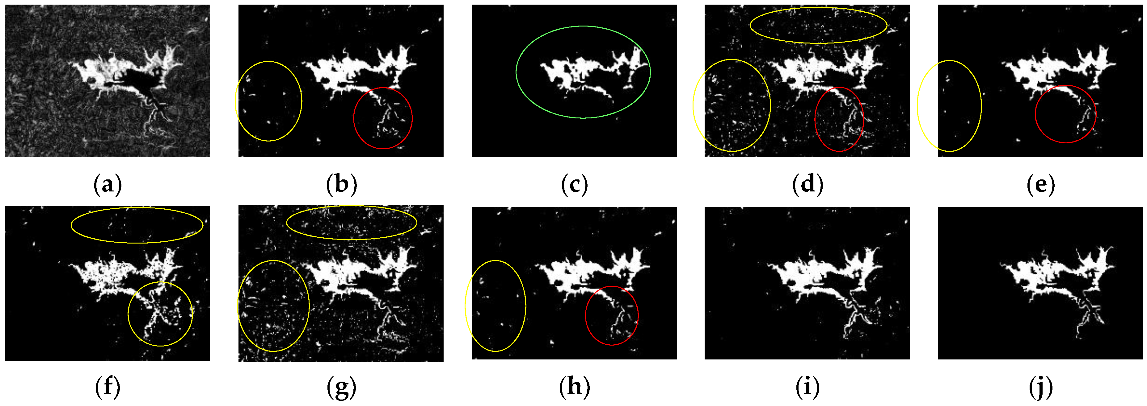
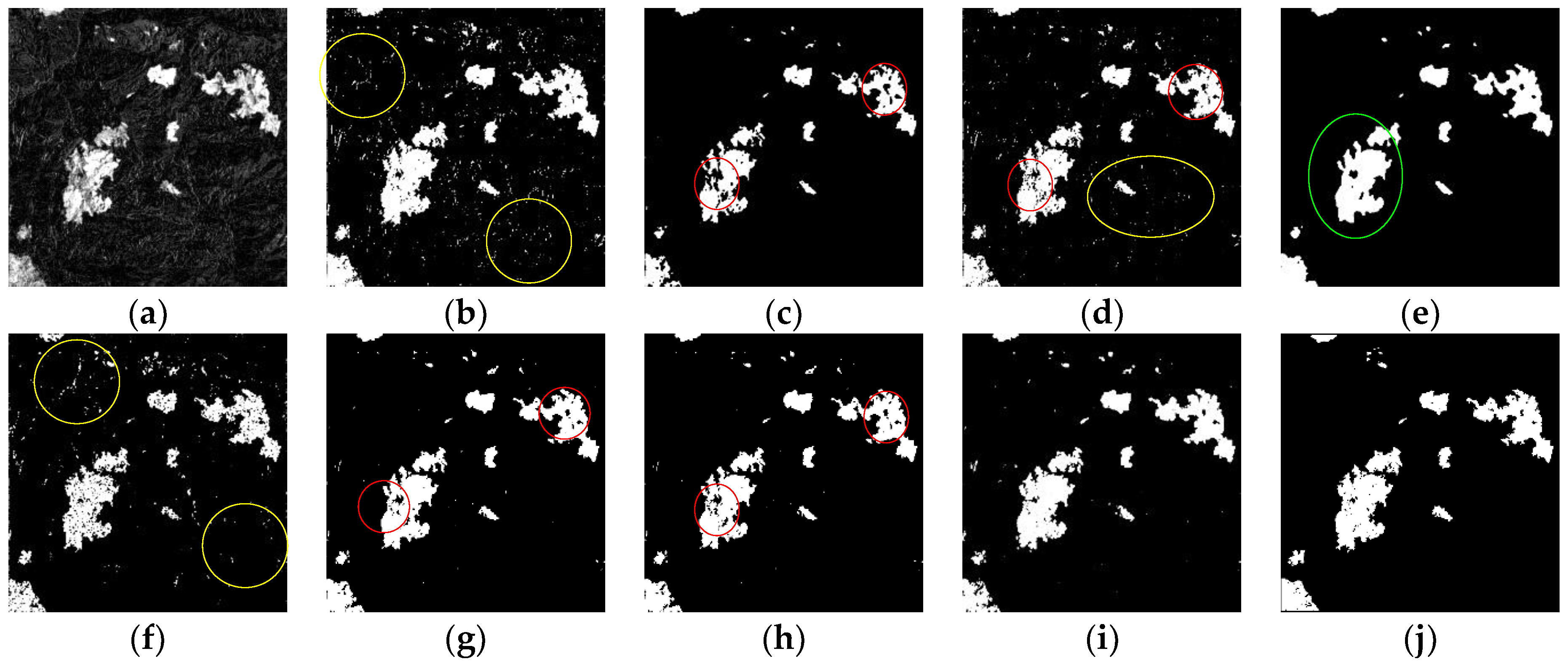
The CMs of the Sardinia dataset are shown in
Figure 9. We can see that the DI (see
Figure 9a) of the Sardinia dataset has some background interference caused by the Gaussian noise. In addition, the lake boundary is weak and slim. Therefore, it is a challenging work to remove the noise while preserving the lake boundary.
We can see that some methods cannot resist the effect of the noise due to ignoring of spatial-contextual information, such as KI (see
Figure 9b), FCM (see
Figure 9d), and GA-mask (see
Figure 9f)), in which many pixels are wrongly detected as changed. MRF+EM (see
Figure 9c) shows a good performance in noise removal, but its CM appears over-smoothing and the weak changed boundary of the lake is not detected. Although the average of the neighborhood pixels has been considered, there are some small false detected regions in the CMs of FLICM (see
Figure 9e), GA-FCM (see
Figure 9g), and MOEA/D (see
Figure 9h). The result of the proposed method is shown in
Figure 9i; it was found that the M-DECD can not only effectively resist background interference and generate a clean CM, but also retain the weak changed boundary of the lake, especially in the red oval regions.
4.3.3. Results of the Alaska Dataset
The results of the Alaska dataset are shown in
Figure 10. In
Figure 10a, we see that the Alaska dataset has complex background interference, caused by both Gaussian noise and local brightness distortion (marked by the blue ovals). In addition, there are many weak and slim edges. Therefore, CD of the Alaska dataset is quite challenging.
As shown in
Figure 10, compared with the reference map (see
Figure 10j), we see that some methods are edge-sensitive, including KI (see
Figure 10b), FCM (see
Figure 10d), and GA-mask (see
Figure 10f). However, these methods are also noise-sensitive, and many pixels are wrongly detected as changed. MRF+EM (see
Figure 10c), FLICM (see
Figure 10e), GA-FCM (see
Figure 10g), and MOEA/D (see
Figure 10h) can reduce some false alarms by considering the spatial information of the neighborhood pixels; however, the spatial smoothness may blur the edges and it cannot resist local brightness distortion. Therefore, these methods misjudge some pixels in brightness distortion regions. Some methods lose many weak changed edges due to over-smoothing (MRF+EM, FLICM, and MOEA/D). The results of the M-DECD are shown in
Figure 10i; it was found that the M-DECD can resist the effect of Gaussian noise and generate a clean CM due to the Wiener de-noised feature. Moreover, the M-DECD performs well in brightness distortion regions due to the structural similarity feature.
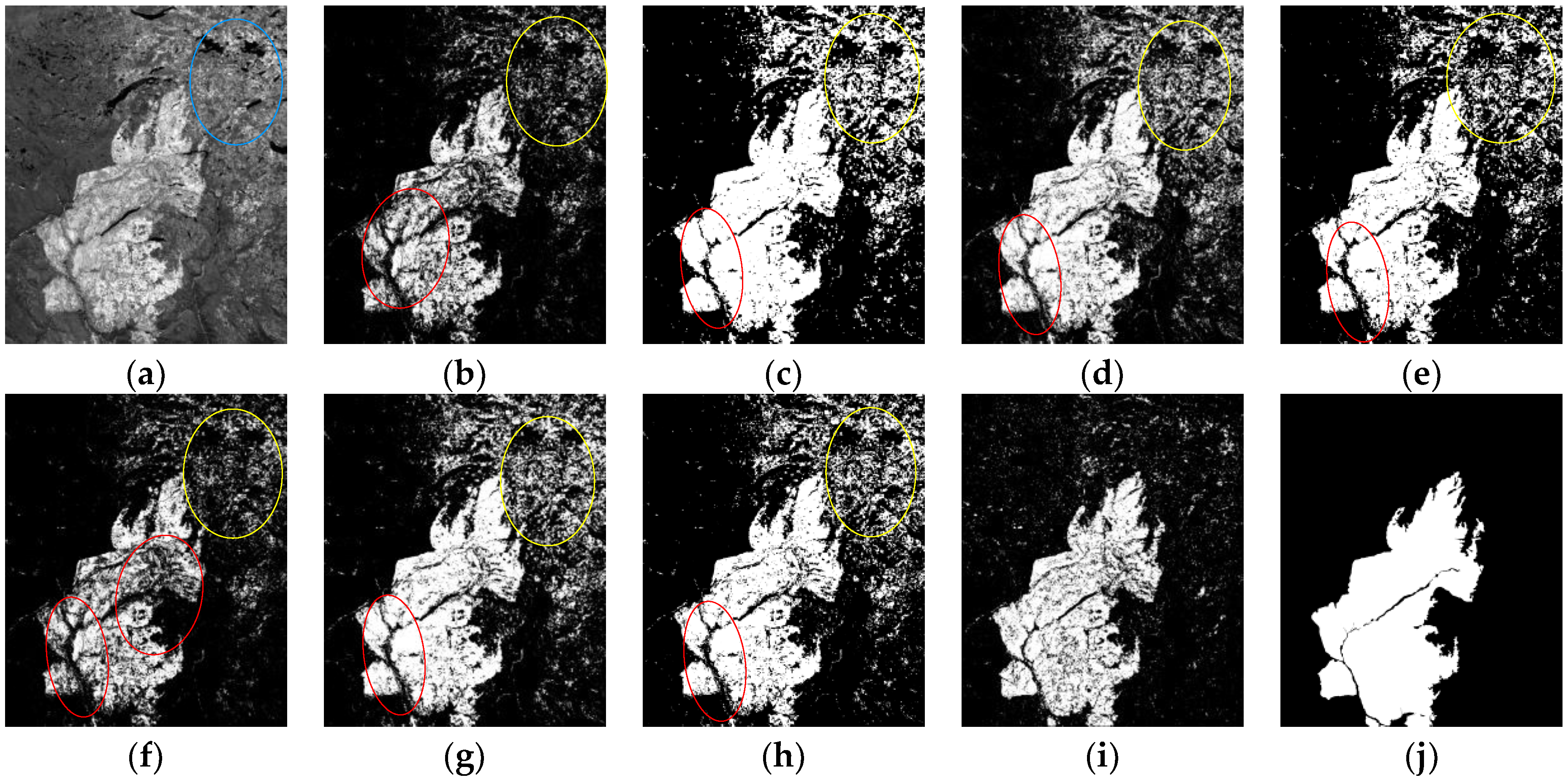
4.3.4. Results of the Canada Dataset
The CMs of the experiments tested on the Canada dataset are shown in
Figure 11. First, the size of the Canada dataset is larger than the other three datasets. In addition, from
Figure 11a, we see that the Canada dataset has strong background interference, caused by both Gaussian noise and local brightness distortion (marked by the blue ovals), especially in the top right corner, where has severe local brightness distortion. Moreover, the spectral contrast between the changed and unchanged regions is low. Therefore, CD of the Canada dataset is the most difficult in our experiments.
As shown in
Figure 11, compared with the reference map (see
Figure 11j), we can see that the advantage of the proposed M-DECD is obvious. Some methods are sensitive to the image noise and local brightness distortion, including KI (see
Figure 11b), FCM (see
Figure 11d), and GA-mask (see
Figure 11f)). However, some other methods can resist the image noise, including MRF+EM (see
Figure 11c), FLICM (see
Figure 11e), GA-FCM (see
Figure 11g), and MOEA/D (see
Figure 11h). However, they cannot resist local brightness distortion, and many regions are wrongly detected as changed, especially in the top right corner of the CMs. The result of the M-DECD is shown in
Figure 11i; it was found that the M-DECD performs well in brightness distortion regions, while preserving the changed details.
4.3.5. Quantitative Analysis
The quantitative evaluation of the experimental results is listed in
Table 4. The optimal results of each evaluation index are marked in bold, and the suboptimal results are underlined.
Among the four datasets, CD of the Mexico dataset is the easiest, and CD of the Sardinia dataset is more difficult due to background noise and weak changed edges. The OE and kappa of M-DECD are very close to the best results, because the FA of M-DECD is a little higher than the best result due to edge expansion, which is caused by the detail enhancement feature. The performance of the M-DECD could be further improved by adopting a more appropriate edge detection method.
CD of the Alaska dataset is quite challenge, due to the complex background interference caused by Gaussian noise and local brightness distortion, and there are many weak changed edges. CD of the Canada dataset is the most difficult, due to its large size and strong brightness distortion caused by illumination difference. The accuracies of the M-DECD on the Alaska dataset and the large Canada dataset increased by about 3.3% and 11.9%, respectively. This indicates that the multi-feature space is suitable for Landsat images and the DE clustering-based CD method is effective.
In addition, we can find that the CD results of the EAs clustering-based CD methods (e.g., GA-FCM, MOEA/D, and M-DECD) perform better than those conventional clustering-based CD methods (FCM, FLICM), which demonstrates the promising optimization capability of the EAs for clustering-based CD. The M-DECD obtains stable results with high accuracy in all of the tested datasets, which proves that adaptive DE algorithm is robust and effective in searching the optimal CD results.
4.4. Experiment Analysis
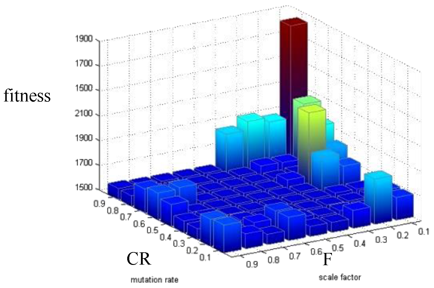
4.4.1. Analysis of the Self-Adaptive Strategy
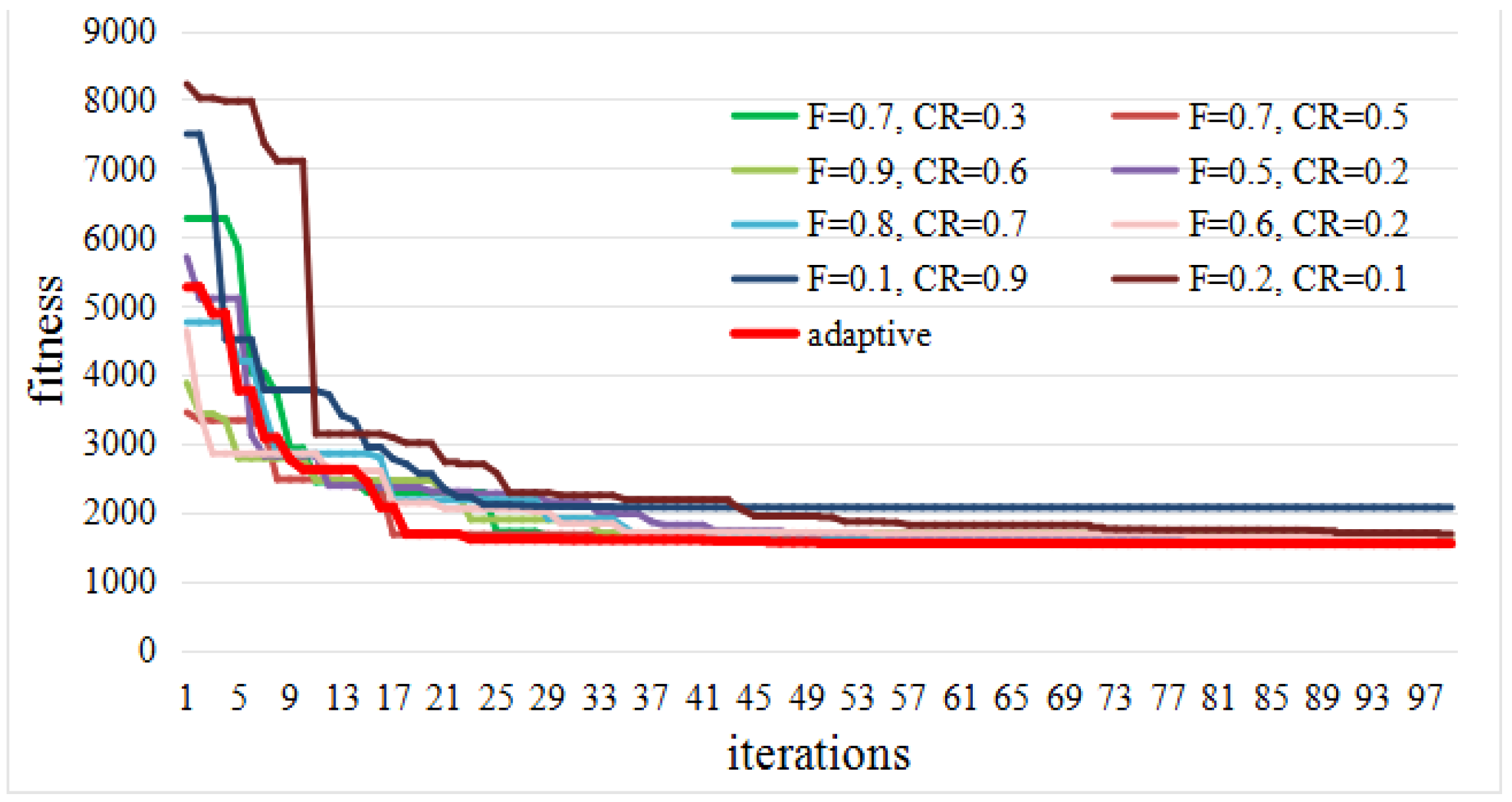
The proposed M-DECD adopted a self-adaptive parameter adjustment strategy [
42] for DE. In order to prove the significance of the adaptive strategy, the relationship between the DE performance and different combinations of control parameters was analyzed. Without loss of generality, the experimental result obtained with the Alaska dataset is presented in
Figure 12. The abscissas are parameters
CR and
F, respectively, and the ordinate is the fitness value of the optimal solution. It can be seen that the different combinations of the control parameters have a significant influence on the optimization result. DE with an inappropriate combination of
CR and
F converges to the local minima, which will affect the detection result. Therefore, it is crucial to use an adaptive strategy to ensure that DE converges to the global optimal solution.
In order to prove the effectiveness of the adopted self-adaptive strategy, we analyzed the relationship between the algorithm convergence process and different combinations of control parameters, as shown in
Figure 13. The abscissa is the number of DE evolutionary iterations, and the ordinate is the fitness value of the optimal solution in each generation. It can be concluded that the adopted strategy (red line) can not only improve convergence speed, but also enhance the robustness of the algorithm.
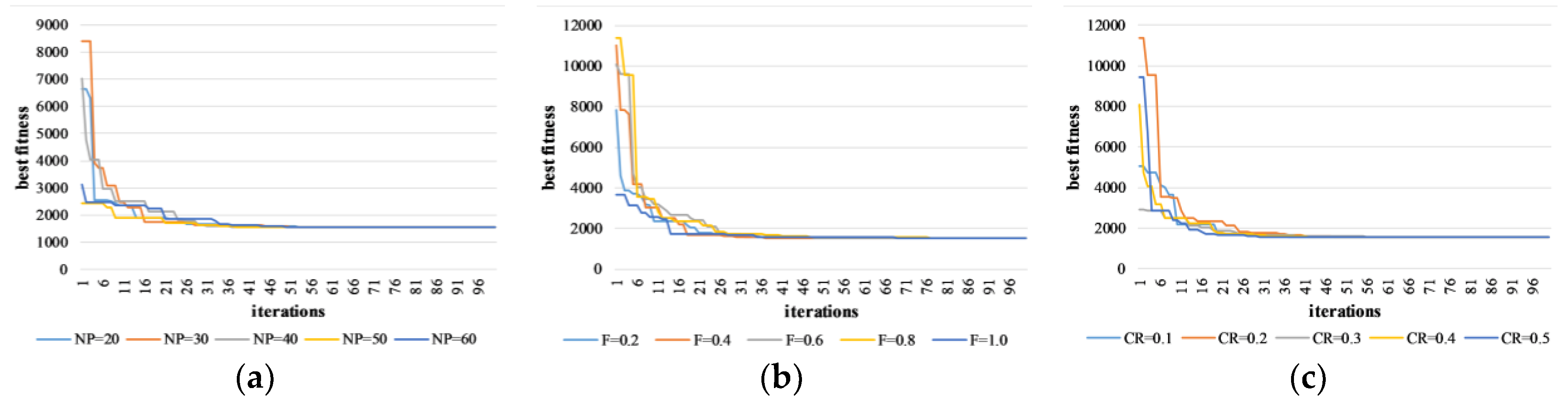
4.4.2. A Sensitivity Analysis on Adaptive DE Algorithm
There are three parameters that have to be set before the adaptive DE-based CD step, i.e., population size
NP, initial scale factor
F0, and initial crossover rate
CR0. In order to prove the robustness of the adaptive DE, we tested the influence of these parameters. Without loss of generality, the tested results of Alaska dataset are shown in
Figure 14. For demonstration purposes, after each generation, we recorded the fitness of the best individual as the Y-axis, i.e., the
Jm distance of the best clusters, and the X-axis is the parameter of DE. Population size is an important parameter, which affects the distribution of population and convergence behavior. We fixed
F0 = 0.8 and
CR0 = 0.2, then recorded the performance of DE at different population sizes, as shown in
Figure 14a. Further, we fixed
NP = 30 and
CR0 = 0.2, and recorded the performance of DE with various initial scale factors, as shown in
Figure 14b. Furthermore,
Figure 14c depicts the performance of DE with different initial crossover rates, where
NP = 30 and
F0 = 0.8.
From the results, it can be concluded that the performance of the adaptive DE algorithm is very stable. The population size NP, initial scale factor F0, and initial crossover rate CR0 have little effect on convergence behavior. On one hand, the optimization of CD clusters is not difficult owing to the low-dimensional encoding strategy. On the other hand, the parameter self-adaptive strategy can dynamically adjust the scale factor and the crossover rate, and improve the search efficiency of DE. Therefore, the adaptive DE algorithm can converge to satisfactory optimization results in 100 iterations under various parameters.
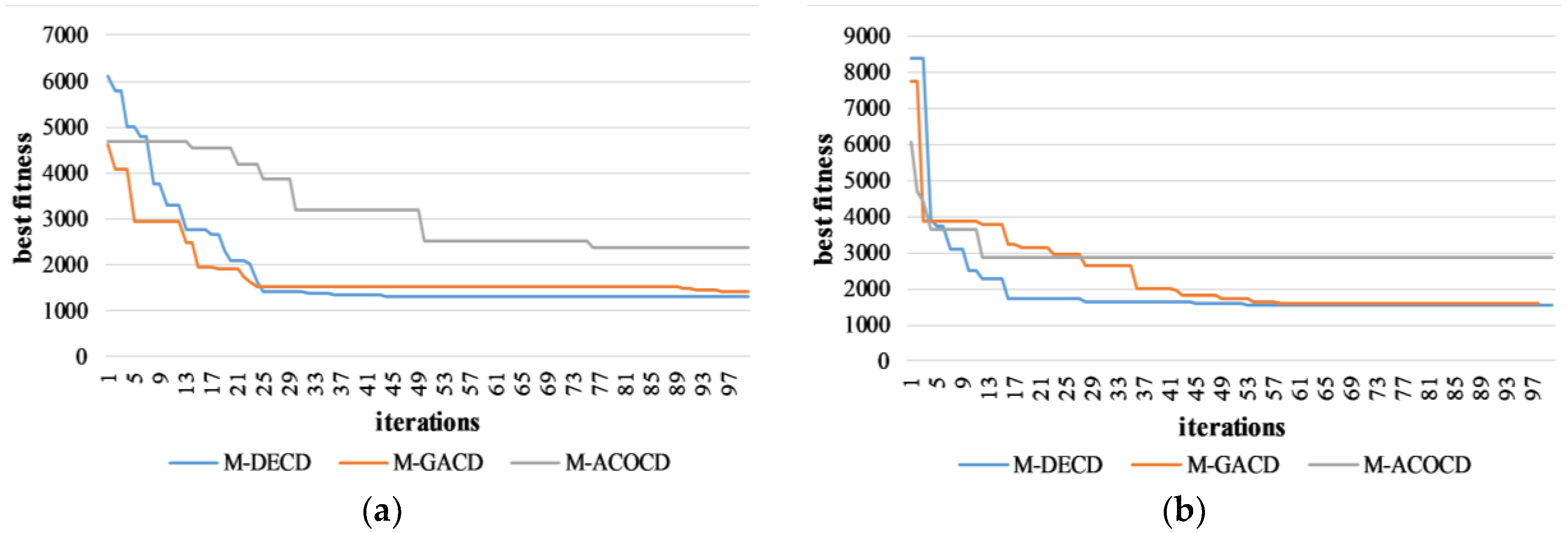
4.4.3. Performance Comparison of GA, ACO, and DE
The DE algorithm is employed to search for the optimal changed and unchanged clusters with minimum
Jm distance. However, DE is just a case study of the proposed optimal multi-feature clustering-based CD framework, and can be replaced by other EAs with powerful optimization ability. In this section, we further test the performance of other EAs, i.e., genetic algorithm (GA [
43]), ant colony optimization algorithm (ACO [
44]) in the proposed framework, namely M-GACD and M-ACOCD. The purpose is to compare the convergence process of GA, ACO, and DE algorithms using the proposed objective function. In the GA algorithm, considering that the individual is encoded with real-value, we use intermediate recombination and real-value mutation operators [
43] to produce new individuals. As for the ACO algorithm, we adopt the real-value mutation operator to construct new solutions, and the transition probability and pheromone are updated according to the basic ACO [
44,
45]. These EAs randomly generate
NP clusters, and evolve the clusters through different evolutionary operators. For fairness, their population size is set to 30, and the maximum number of generations is set to 100. The Sardinia dataset and the Alaska dataset are selected as examples, and
Figure 15 depicts the convergence process of the compared EAs. The abscissa is the number of generations, and the ordinate is the best fitness of the optimal clusters in each generation.
From the results of the Sardinia dataset and the Alaska dataset, we find that the initial populations of GA and ACO are better than DE, because the populations are randomly generated. However, eventually, the DE algorithm converges to the best solution with minimal fitness, which demonstrates that DE has a powerful global search capability. The GA algorithm can obtain a better solution than the ACO algorithm. Since the ACO algorithm is more suitable for combinatorial optimization, such as the traveling salesman problem [
46], the proposed CD problem is a continuous optimization problem, so the ACO algorithm tends to fall into the local minima, resulting in failure to find optimal clusters.
4.4.4. Robustness Test
Taking into consideration interferences in the Landsat image, three features are extracted to construct a multi-feature space—detail enhancement, Wiener de-noising, and structural similarity. In this section, we test the robustness of the proposed M-DECD in resisting the interferences of the Landsat images, and analyze the effect of the three features.
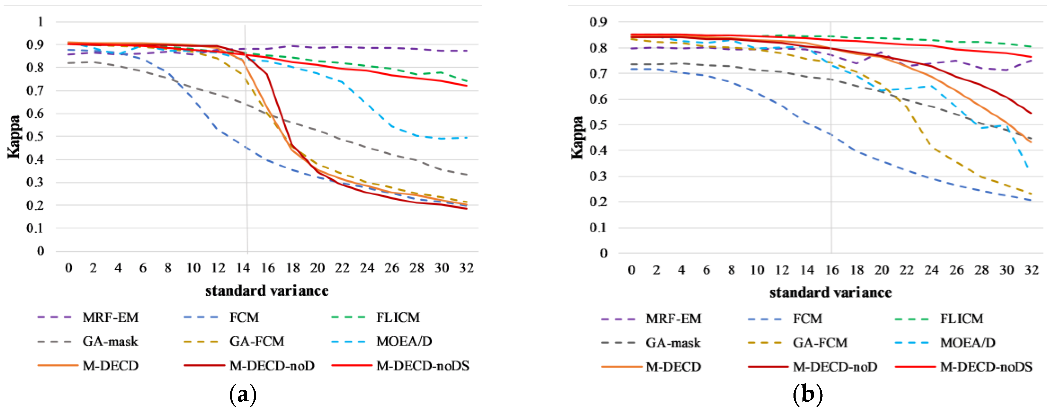
The Mexico dataset and the Sardinia dataset are selected for the Gaussian noise robustness test, because the background interference of the two datasets is mainly composed of Gaussian noise with little brightness distortion. The Gaussian noise, which obeys the normal distribution
, is added into the tested datasets. The accuracy (Kappa coefficient) of the comparison methods is recorded as the Y-axis, and the X-axis is the standard variance of the Gaussian noise, as shown in
Figure 16. It can be found that the MRF-EM and FLICM methods can remove strong Gaussian noise, because their CD is conducted with spatial information derived from the neighborhood pixels in DI. Although the proposed M-DECD method has employed the Wiener filter to remove some Gaussian noise, the detail enhancement feature strengthens the interference when the noise is too strong (
σ > 14 for the Mexico dataset and
σ > 16 for the Sardinia dataset), resulting in reduced accuracy. Therefore, we further tested the M-DECD method without the detail enhancement feature and the M-DECD method only with the Wiener de-noise feature, namely M-DECD-noD and M-DECD-noDS, respectively. We found that the M-DECD-noDS can obtain similar results as the FLICM when the noise is strong. The M-DECD-noD performs better than M-DECD, but it still cannot resist strong image noise, which means the structural similarity feature also enhances the image noise to some extent. Thus, the proposed method could be further improved by combining the multiple features in a more appropriate way.
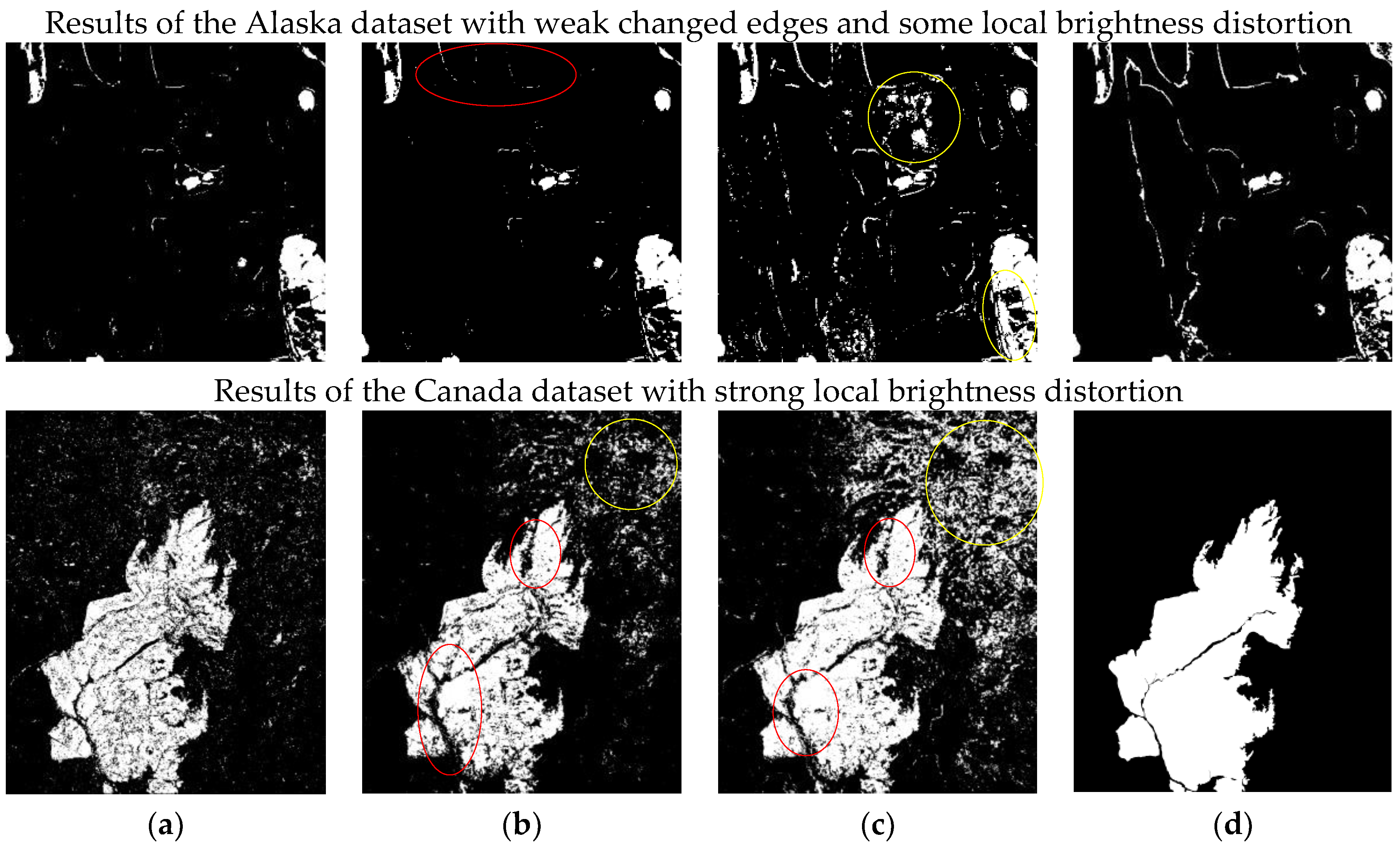
Furthermore, the Alaska dataset and the Canada dataset are tested to prove the effectiveness of the detail enhancement feature and the structural similarity feature, because the Alaska dataset has many weak changed edges and some local brightness distortion, while the Canada dataset is affected by stronger local brightness distortion (marked by the blue ovals in
Figure 11a). For demonstration, we tested the M-DECD method without the detail enhancement feature (M-DECD-noD) to analyze the effect of detail preservation, and we also tested the M-DECD without structural similarity feature (M-DECD-noS) to analyze the robustness of the algorithm to local brightness distortion. The CMs are depicted in
Figure 17 and their accuracy is listed in
Table 5.
The CMs of the Alaska dataset show that the M-DECD-noD lost some weak changed edges (marked by red oval), compared to the M-DECD, which indicates that the M-DECD has better detail preservation ability due to the detail enhancement feature. The multi-feature space of M-DECD-noS is composed of the detail enhancement feature and the Wiener de-noise feature; thus, its CM contains several changed details. However, without the structural similarity feature, the CM of M-DECD-noS has many false detected pixels in the brightness distortion region (marked by yellow oval). From the CMs of the Canada dataset, we find that the M-DECD-noD and the M-DECD-noS miss a lot of changed pixels, which prove that the detail enhancement feature and the structural similarity feature can preserve local details of the changed object. Since the spectral contrast between the changed and unchanged regions is low in the Canada dataset, it needs as much information as possible for the accurate CD. The M-DECD-noD does not consider the spectral value of DI, so its CM has some false detected pixels in the right top corner. On comparing the CMs of the M-DECD and the M-DECD-noS, we can conclude that the structural similarity feature is effective in resisting strong local brightness.
The accuracy of the M-DECD and M-DECD-noD demonstrates that the detail enhancement feature can decrease the miss alarm, and the accuracy of the M-DECD and M-DECD-noS proves that the structural similarity feature can significantly decrease the false alarm, especially when the interference of images is mainly caused by local brightness distortion.
5. Discussion and Conclusions
In this paper, we proposed an unsupervised CD method based on multi-feature clustering using adaptive differential evolution (M-DECD) for Landsat imagery. The proposed method constructs an effective multi-feature space for Landsat image CD, which can resist Gaussian noise and local brightness distortion, while preserving weak changes. Three features are extracted from the multi-temporal images and DI—Wiener denoising, detail enhancement, and structural similarity. In order to obtain optimal CD results, the M-DECD combines the DE algorithm with FCM to search the changed and unchanged clusters in the multi-feature space by minimizing the Jm distance. In addition, the control parameters of the DE algorithm have been adaptively adjusted to improve the robustness of M-DECD. Four Landsat datasets with typical natural land cover changes have been tested and the experiment results demonstrate the effectiveness and superiority of the M-DECD when compared with seven conventional and state-of-the-art methods, especially for the Canada dataset, whose detection accuracy is increased by 11.9%.
However, the proposed method treats all the features equally. It could be further improved by analyzing the noise level and brightness distortion level of the data, then incorporating the multiple image features in a more appropriate way. In addition, the detail enhancement feature strengthens image noise, so the M-DECD is not suitable for processing SAR image with strong speckle noise.


