Vegetation Optical Depth and Soil Moisture Retrieved from L-Band Radiometry over the Growth Cycle of a Winter Wheat

Abstract

L-band radiometer measurements were performed at the Selhausen remote sensing field laboratory (Germany) over the entire growing season of a winter wheat stand. L-band microwave observations were collected over two different footprints within a homogenous winter wheat stand in order to disentangle the emissions originating from the soil and from the vegetation. Based on brightness temperature (T_B) measurements performed over an area consisting of a soil surface covered by a reflector (i.e., to block the radiation from the soil surface), vegetation optical depth (τ) information was retrieved using the tau-omega (τ-ω) radiative transfer model. The retrieved τ appeared to be clearly polarization dependent, with lower values for horizontal (H) and higher values for vertical (V) polarization. Additionally, a strong dependency of τ on incidence angle for the V polarization was observed. Furthermore, τ indicated a bell-shaped temporal evolution, with lowest values during the tillering and senescence stages, and highest values during flowering of the wheat plants. The latter corresponded to the highest amounts of vegetation water content (VWC) and largest leaf area index (LAI). To show that the time, polarization, and angle dependence is also highly dependent on the observed vegetation species, white mustard was grown during a short experiment, and radiometer measurements were performed using the same experimental setup. These results showed that the mustard canopy is more isotropic compared to the wheat vegetation (i.e., the τ parameter is less dependent on incidence angle and polarization). In a next step, the relationship between τ and in situ measured vegetation properties (VWC, LAI, total of aboveground vegetation biomass, and vegetation height) was investigated, showing a strong correlation between τ over the entire growing season and the VWC as well as between τ and LAI. Finally, the soil moisture was retrieved from T_B observations over a second plot without a reflector on the ground. The retrievals were significantly improved compared to in situ measurements by using the time, polarization, and angle dependent τ as a priori information. This improvement can be explained by the better representation of the vegetation layer effect on the measured T_B.

1. Introduction

Soil surface moisture is a key variable in the hydrological cycle, and global information on soil moisture can improve our knowledge about heat and mass exchange at the land–atmosphere interface. Furthermore, information on vegetation properties is of great interest to characterize plant dynamics and crop stands within and between seasons globally. L-band (1–2 GHz) microwave radiometry is a promising technique to retrieve and monitor soil surface moisture and vegetation properties simultaneously. The main reasons for using L-band radiometry compared to higher microwave frequencies include: the semi-transparence of the vegetation layer; the deeper depth of soil emission; the lower sensitivity to scattering within the vegetation canopy; and the reduced effect of the soil surface roughness on the measured microwave signal [1,2]. Additionally, most L-band radiometer systems operate at 1.4 GHz frequency (λ ~ 21 cm), because this frequency lies within a protected frequency band, where radio frequency interferences (RFI) are limited. However, the vegetation layer attenuates the L-band microwave emission originating from the soil and contributes its own emission, enabling simultaneous measurement of the soil and vegetation. Yet, it remains challenging to disentangle the emissions originating from the soil and the vegetation [3,4]. Currently, two L-band satellite missions are in operation, namely, the Soil Moisture and Ocean Salinity (SMOS) satellite mission launched by the European Space Agency (ESA) in 2009 [5], and the Soil Moisture Active Passive (SMAP) satellite mission launched by the National Aeronautics and Space Administration (NASA) in 2015 [6,7]. Both missions aim to provide global soil moisture products with a high temporal resolution (2–3 days) and high retrieval accuracy (≤0.040 m³ m⁻³) [8].

Unfortunately, satellite missions are still limited in their spatial resolution (>10 km), and therefore, process studies looking at specific effects such as the effect of soil surface roughness, topography, or the vegetation canopy on spaceborne brightness temperature observations are hardly feasible. To overcome this limitation, tower-based radiometer measurements are still needed to improve our process understanding and to develop and validate radiative transfer models (e.g., [9,10,11]). In particular, the effect of the vegetation layer on the L-band emissions is of uppermost importance to improve the soil moisture retrieval and enable vegetation observations from L-band brightness temperature data. Currently, different radiative transfer (RT) models with varying complexities are in use to account for the attenuation effects in vegetation layers on L-band brightness temperature (T_B) observations. The non-coherent τ-ω model, which is a zero-order solution of the RT equations, is the most commonly used model [8,12,13]. The τ-ω model describes the attenuation of the microwave radiations by the vegetation layer using the vegetation optical depth parameter (τ) and accounts also for the scattering within the vegetation canopy using the effective scattering albedo (ω) parameter. Both parameters may depend on the vegetation structure and are not constant over a growing season. However, their respective influence on the microwave emissions is not yet fully understood. To investigate their influence on the soil microwave emission in order to improve the soil moisture retrieval, several studies have already been performed using field-scale (e.g., [11,13,14,15]) or air- and spaceborne L-band radiometer measurements (e.g., [16,17,18,19,20]).

In the retrieval algorithms currently used, the τ parameter is typically retrieved simultaneously with the soil moisture, as in the SMOS algorithm (or the SMAP dual-channel algorithm (SMAP DCA) and the SMAP multi-temporal dual-channel algorithm (SMAP MT-DCA)), or estimated from ancillary data such as MODIS NDVI in the SMAP single-channel algorithm (SMAP SCA)) [8,21]. Independently of the retrieval scheme, τ is assumed to be polarization and angle independent for both spaceborne platforms [22], whereby several studies performed with ground-based radiometers have indicated a polarization- and angle-dependent τ (e.g., [3,23,24,25]). However, none of the above-listed experiments studied a complete growing season, and therefore, the conclusions drawn are still incomplete.

This study aims to further improve the understanding on the attenuation of the vegetation layer on the L-band emissions and to enhance the soil moisture retrieval using microwave radiometer measurements. First, special attention was set to the analysis of the time, polarization, and angle dependency of the τ parameter. Second, the focus was set on the investigation of the impact of the quality of the τ parameter on the soil moisture retrieval. Finally, the relationship between the radiometer-derived τ and several vegetation indices measured during the field campaign was analyzed.

To this end, a tower-based experiment was performed at the Selhausen remote sensing field laboratory (Germany) over the entire growing season of a winter wheat canopy between the 10th of April and 14th of August 2017. To disentangle the vegetation emission from the soil emission, radiometer measurements took place over two footprint types within the same winter wheat stand (i.e., a plot with the soil covered by a reflector (metal grid) with the vegetation growing through, and a plot covered only by vegetation) using different incidence angles. To analyze if the time, polarization, and angle dependence of τ is also highly dependent on the observed vegetation species, white mustard was grown during summer 2016, and radiometer measurements were performed using the same experimental setup, but with lower incidence angles (Section 2). These measurements were accompanied by in situ measurements of the soil and vegetation status (Section 4.1). The retrieval of the soil moisture and vegetation optical depth was performed using the τ-ω model (Section 3). In a first step, τ was retrieved from the T_B measured over the gridded area (i.e., allowing T_B measurements of the vegetation alone) to investigate the temporal, polarization, and angle dependencies of τ. In a second step, the relationship between vegetation optical depth and in situ measured vegetation properties (VWC, LAI, TOB, and vegetation height) will be presented. Finally, these τ parameters were used as a priori information in the soil moisture retrieval based on the T_B measured over the non-gridded area. To validate the improvement in the soil moisture retrieval using a time-, polarization-, and angle-dependent τ as a priori information, other retrieval schemes were also formulated, where τ was simultaneously estimated during the soil moisture retrieval (Section 4.2, Section 4.3, Section 4.4 and Section 4.5). This is followed by a discussion on the τ and soil moisture estimates in comparison to other studies at the field and global scale (Section 5). In Section 6, a conclusion will be provided.

2. Field Setup and Instrumentation

The experiment was performed at the Selhausen remote sensing field laboratory (Germany), which is located within the Rur river catchment. A picture of the setup is shown in Figure 1a. The soil type is a silt loam according to the United States Department of Agriculture (USDA) textural classification with 13% sand, 70% silt, and 17% clay. Total organic carbon and total nitrogen contents of the plough layer are 1.01 and 0.102 mass %, respectively. More detailed information about the site characteristics can be found in [26].

Within this test site, an experimental plot with an area of 0.05 ha (12 m wide and 40 m long) was established. One part of the experimental area consisted of a soil covered by a reflector (metal grid) with vegetation growing through (gridded or reflector plot) and the other plot consisted of a vegetated area without a reflector on the soil (non-gridded plot) (Figure 1b). The mesh size of the reflecting grid was <1 cm to achieve a highly reflecting surface, disturbing neither hydrology nor plant growth. By using this experimental approach, it was possible to measure the L-band microwave emission of the vegetation layer alone, while the emission from the underlying soil was blocked by the reflecting grid [27,28].

L-band passive microwave remote sensing measurements were performed with the ELBARA-II radiometer at a frequency of 1.4 GHz. The measurements were performed at horizontal (p = H) and vertical (p = V) polarization (p) using a 3 s integration time to provide an accuracy of about 1 K. The radiometer was attached to a dual-mode conical horn antenna (60 cm in diameter and 67 cm long) with symmetrical and identical beams and a −3 dB full beam width of 23° in the far field. A detailed description of the technical specifications of ELBARA-II can be found in [11] and [29], as well as the internal and external calibrations used to retrieve the brightness temperatures (T_B) from the radiometer raw data. The radiometer was mounted at about 4 m height on a moving platform (aluminum bridge) (Figure 1a), which was moved between the gridded and non-gridded plot (the two orange rectangles in Figure 1b depict the exact bridge positions). T_B measurements were repeated twice a week at incidence angles (θ) ranging between 40° and 60° in increments of 5° above the non-gridded and gridded plots. Each T_B measurement was performed for 20 min using a 5 min interval (equal to 5 measurements per angle). In between these bi-weekly measurements, the bridge was located permanently at the non-gridded plot and T_B measurements were performed every 5 min using a 40° angle only.

Additionally, in situ sensors were installed to monitor the soil relative dielectric permittivity (ε_S), the soil temperature (T_S), and the vegetation canopy temperature (T_C) at both plots. As the relative dielectric permittivity is a complex number, ε_S refers to its real part. The test site was equipped with 30 5TM/TE capacitance sensors (Decagon Devices, Pullman, WA) installed horizontally at 5 cm depth and with the plane of the sensors parallel to the soil surface. The sensors were installed at the two radiometer measurement locations with 15 sensors each located within the 40°, 45° and 50° radiometer footprints (Figure 1b). These sensors measured the ε_S and T_S every 15 min, which were logged with an ECH₂0 Em50 logger (Decagon Devices, Pullman, WA, USA). The sensing volume can be expected to be maximum 515 cm³ in a dry soil, and smaller in a wetter soil, along the three prongs of 5.2 cm length. Volumetric soil water content (SWC) data were derived from the in situ ε_S measurements using a soil-specific calibration relation obtained in the laboratory. For this purpose, soil was taken from the top soil layer (i.e., 0–5 cm depth) at the center of the test site, and air dried to a SWC of about 0.04 m³ m⁻³ and passed through a 2 mm sieve in the laboratory. Then, 10 kg of dry soil were packed in a box (36.8 cm long × 26.8 cm wide × 17 cm high) in order to obtain a bulk density of about 1.52 g cm⁻³, which is similar to the soil bulk density observed at the test site. Ten sensors were installed at 3 cm depth horizontally and parallel to the soil surface within the soil. The whole setup was placed on a scale to monitor the soil water content. The soil was first wetted stepwise to full saturation (SWC of about 0.42 m³ m⁻³). Then, the soil was exposed to evaporation and dried out continuously to values below 0.04 m³ m⁻³, whereby the ε_S was derived from the sensor measurements and the SWC was calculated by the weight loss of the soil. Using pairs of measured ε_S and SWC, the following site-specific equation was obtained:

$$SWC=-0.1166+0.0213{\epsilon }_{\mathrm{S}}+0.0005{\epsilon }_{\mathrm{S}}^2\left({\mathrm{R}}^2=0.99\right),$$

(1)

In addition to the 30 5TM/TE capacitance sensors, 30 custom-made time-domain reflectometry (TDR) sensors were installed horizontally and parallel to the soil surface at 30 cm depth within the soil along a transect at the non-gridded plot to measure ε_S. The sensors were connected to a Campbell TDR100 and CR1000 data logger (Campbell Scientific, Logan, UT, USA) using six 50C81-SDM multiplexers. The TDR measurement interval was set to 30 min. Air temperature within the vegetation canopy was measured at different heights (15, 30, 45, 60, 75 and 90 cm above ground) for the non-gridded and gridded plot using twelve Pt100 sensors (six for each plot) with an accuracy of about 0.1 °C. The measuring interval was set to 5 min and the data were logged with a DT85 logger (COSINUS Messtechnik GmbH, Taufkirchen, Germany).

Furthermore, information about precipitation and air temperature (T_A) were taken from the TERENO climate station (SE_BDK_002, http://teodoor.icg.kfa-juelich.de/observatories/ELRV_Observatory/) located at the border of the Selhausen remote sensing field laboratory. Soil surface roughness was measured at the beginning of the experiment (3 April) along a transect in the radiometer viewing direction using a custom-made laser scanner system 1 m in length (Institute of Geography, University of Cologne, Germany), which measured the absolute distance from the soil.

Winter wheat (Triticum aestivum L.) was sown on 4th of November 2016 with a seeding density of 160 kg ha⁻¹ (equal to 300 seeds per m²). The row spacing was 14 cm. Before sowing, the soil was tilled to a depth of about 10 cm using a plough and the seedbed was prepared using a ground driven harrow. The alignment of the vegetation rows and the plough direction was parallel to the direction of the radiometer measurements. The winter wheat was harvested on the 14th of August 2017 during late senescence. It has to be noted that, for comparison, information collected during a short experiment performed in summer 2016 using the same experimental setup, but less incidence angles, will be used later in Section 4. During this short experiment, white mustard (Sinapis alba L.) was sown manually on the 27th of June 2016 with a seeding density of 80 kg ha⁻¹ (equal to 500 up to 1600 seeds per m²). The row spacing varied between 5 and 10 cm, and the soil surface was also tilled to a depth of about 10 cm using a plough, as well as being tilled manually using a rake to a depth of about 3 cm to reduce the surface roughness. The mustard plants were harvested on the 21st of September 2016 shortly before the beginning of the senescence.

Furthermore, vegetation characteristics were gathered over the entire growing season of the winter wheat. Therefore, the leaf area index (LAI), total of aboveground biomass (TOB), which is the mass of dry vegetation per ground area, vegetation water content (VWC), which is the mass of water in the vegetation per ground area, growing stages, and vegetation height were measured in the plots, but outside the radiometer footprints. LAI, TOB, and VWC were measured destructively every week during the vegetation period after the plants were cut from an area of about 0.33 m². To measure the LAI, the vegetation samples were scanned in the laboratory using the LI-3000 C Area Meter (Li-COR, Lincoln, NE, USA). For the TOB and VWC measurements, the plants were dried for 48 h at 65 °C and weighed before and after the drying. Growing stages were defined according to the Biologische Bundesanstalt, Bundessortenamt und CHemische Industrie (BBCH) scale, which describes the morphological development of a plant with a decimal code using values ranging from 0 to 99, as described in Lancashire et al. [30] based on the Zadoks code for cereals [31]. The height was measured at six representative points within the test site plots during the vegetation destructive samplings and with a fixed camera system (Wild Vision Full HD 5.0) using a reference scale bar placed on the side opposite to the camera position. Another camera was placed on the bridge to monitor any structural changes within the observed footprints. Both cameras took pictures every six hours.

3. Radiative Transfer Model

3.1. Model Description

For soil surfaces with low vegetation, such as grass or crop stands, the non-coherent tau-omega (τ-ω) model, which is a zero-order solution of the radiative transfer (RT) equations, is the most commonly used approach to describe the brightness temperature observed at L-band [8,14]. When a vegetation layer is covering the soil surface, the vegetation attenuates the microwave emission originating from the soil and, on the other hand, adds its own contribution to the overall emission captured by the L-band radiometer. Two parameters are used in the τ-ω model to account for the influence of the vegetation layer on the emissions originating from the soil and vegetation, namely, the vegetation optical depth (τ) and the effective scattering albedo (ω), which can both be assumed to be polarization (p) dependent. The τ parameter describe the attenuation of the microwave emission by the vegetation layer and ω accounts for the scattering effects within the vegetation layer (volume scattering) in the forward direction, while neglecting multiple scattering [12,13]. In Figure 2, a schematic sketch of the τ-ω model is shown.

The brightness temperature (T_Bp) of a vegetated footprint can be described as:

$$T_{\mathrm{B}p}=\left(1-{\mathsf{\omega }}_p\right)\left(1-{\gamma }_p\right)T_{\mathrm{C}}+\left(1-{\mathsf{\omega }}_p\right)\left(1-{\gamma }_p\right){\gamma }_p{R}_p{T}_{\mathrm{C}}+\left(1-R_p\right){\gamma }_p{T}_{\mathrm{S}},$$

(2)

where ω_p represents the effective vegetation scattering albedo [-], T_C and T_S are the effective vegetation canopy and soil temperatures [K], respectively, R_p is the soil surface reflectivity [-], and γ_p is the vegetation attenuation factor (or vegetation transmissivity) [-].

In this study, ω was assumed to be equal to zero for both polarizations. This is in agreement with the assumption made in the current SMOS algorithm for croplands [8].

The vegetation attenuation factor in Equation (2) is related to τ and the incidence angle (θ) using Beer’s law:

$${\gamma }_p=exp\left(-\frac{{\mathsf{\tau }}_p}{\cos \left(\mathsf{\theta }\right)}\right).$$

(3)

A polarization dependent τ parameter can also be defined as a function of the incidence angle (θ) and the vegetation optical depth at nadir angle, i.e., corrected for anisotropy (τ_NAD) using:

$${\mathsf{\tau }}_p={\mathsf{\tau }}_{\mathrm{NAD}}\left({\sin }^2\left(\mathsf{\theta }\right)t{t}_p+{\cos }^2\left(\mathsf{\theta }\right)\right),$$

(4)

where tt_p is the angular correction factor also at p (H or V) polarization. Due to the dominant vertical structure of the winter wheat plants the tt_H parameter can be set equal to 1 (corresponding to isotropic conditions at H polarization). The tt_V parameter is expected to change during the growing season with values > 1, corresponding to anisotropic conditions at V polarization.

The soil surface reflectivity (R_p) was calculated using Fresnel equations as a function of the soil relative dielectric permittivity (ε_S). In the particular case of the gridded plot, R_p was assumed to be equal to 1, as the grid covering the soil surface represents a perfect reflector.

To account for the soil surface roughness effect on the measured L-band emission, the semi-empirical model of Wang and Choudhury [32], modified by Escorihuela et al. [33] and Wigneron et al. [34], can be used:

$$R_p=\left[\left(1-Q\right)R_{\mathrm{F}p}\left(\mathsf{\theta }\right)+Q{R}_{\mathrm{F}p}\left(\mathsf{\theta }\right)\right]exp\left[-h\cos {\left(\mathsf{\theta }\right)}^n\right],$$

(5)

where R_Fp is the Fresnel reflectivity at p polarization calculated using Fresnel equations; h is the effective surface roughness parameter, where a higher value corresponds to a larger soil surface roughness [-]; Q is a polarization coupling factor due to the fact that soil roughness tends to induce polarization mixing; and n is an integer value to parameterize the dependence of the roughness effect on the incidence angle. Several assumptions can be made for the h, Q, and n parameters of the so-called “HQN” model. The h parameter was set to zero, as the soil surface can be assumed as smooth during the experiment like in general for crop covered surfaces [23]. Indeed, a standard deviation of the soil surface heights lower than 5 mm was measured by a laser scanner system at the beginning of the experiment. Q can be assumed to be equal to zero in this study and the n parameter can be also neglected as the h parameter was set to zero [35,36]. Using the above-mentioned assumptions, the soil surface was considered to be a specular surface; R_p was thus only governed by the Fresnel equations.

Finally, the generalized refractive mixing dielectric model (GRMDM) of Mironov et al. [37] was used to calculate the soil relative dielectric permittivity as a function of soil moisture, soil temperature, and clay content.

3.2. Retrieval Algorithm

In this study, the τ-ω model was first used to retrieve τ from the T_B data collected over the gridded plot and then used to retrieve SWC from the T_B data recorded over the non-gridded plot based on different retrieval schemes. For the τ retrieval, optimal values for τ were estimated for each measurement angle separately (single-angle approach) and also using all angles at the same time (multi-angle approach). For this, T_B data at both polarizations were inverted together. Additionally, information on canopy temperature was used. The T_B data consisted of mean values of the 5 measurements performed per day (n = 33 days) at each incidence angle and for each polarization. For the single-angle approach, τ_H and τ_V were simultaneously inverted within the parameter range [0–3], while for the multi-angle approach, τ_NAD and tt_V were estimated within the parameter ranges [0–3] and [1–15], respectively. The inversions were performed with the multi-level coordinate search (MCS) algorithm, being a global optimization tool as introduced by Huyer and Neumaier [38]. The objective function was defined as the cumulative squared error between the measured and modeled T_B data. In addition, the error between the measured and modeled T_B data was normalized by dividing it by the measured T_B. Optimal values of τ_H and τ_V or τ_NAD and tt_V can be then obtained after finding the minimum of the objective function. The corresponding τ products were analyzed with regard to their time, polarization, and angle dependencies and were used as a priori information to retrieve the SWC from the T_B observations over the non-gridded plot.

For the SWC retrieval, the MCS optimization algorithm was also used. Here, the volumetric soil water content was estimated from T_B observations performed over the non-gridded plot by inverting the τ-ω model and using both polarizations together. Here again, T_B data consisted of mean values of the 5 measurements performed per day (n = 33 days) at each incidence angle and for each polarization. Four different inversion schemes were developed to investigate the impact of a time, polarization, and angle-dependent τ on the soil moisture estimation in comparison to the simultaneous retrieval of τ and SWC. The retrieval schemes, estimated parameters, parameter ranges, and model inputs are depicted in

Table 1. Different retrieval schemes used to estimate the volumetric soil water content (SWC) [m³ m⁻³] from the brightness temperature (T_B) measurements over the non-gridded plot using the τ-ω model.

Retrieval Schemes	Estimated Parameters	Parameter Ranges	Inputs
1-P	SWC	[0.03–0.42]	τH, τV, ω, TBH, TBV, TC, TS
2.1-P	SWC, ω	[0.03–0.42], [0–0.6]	τH, τV, TBH, TBV, TC, TS
2.2-P	SWC, τ	[0.03–0.42], [0–3]	ω, TBH, TBV, TC, TS
3-P	SWC, τNAD, ttV	[0.03–0.42], [0–3], [1–15]	ω, TBH, TBV, TC, TS

. The approaches are namely the 1-P retrieval scheme, where only SWC was inverted, the 2.1-P retrieval scheme where SWC and ω were inverted, the 2.2-P retrieval scheme where SWC and a polarization independent τ were inverted, and the 3-P retrieval scheme where SWC, τ_NAD, and tt_V were inverted, simultaneously. During the 1-P and 2.1-P retrieval schemes the τ parameter was assumed to be known from the inversion of the T_B measurements over the gridded plot, while during the 2.2-P and 3-P retrieval schemes the τ was considered unknown. In all cases, the temperatures of the soil (T_S) and of the vegetation (T_C) were assumed to be known from the in situ measurements. All inversions were performed over a relatively large parameter range (0.03 < SWC < 0.42 m³ m⁻³; 0 < ω < 0.6; 0 < τ < 3; 0 < τ_NAD < 3; 1 < tt_V < 15) to ensure that the global optimum can be found. The inversion schemes 1-P till 2.2-P were conducted for the single- and multi-angle approach, while the 3-P approach was conducted for the multi-angle approach only, as one angle (and two polarizations) does not contain enough information to retrieve more than 2 parameters at the same time. Concerning the single-angle approach, the SWC optimal values and other inverted parameters were retrieved from the T_B data at 40° incidence angle only, as it gives the closest fit between the measured and modeled SWC. For the multi-angle approach, all available angles were used for the retrieval.

4. Results

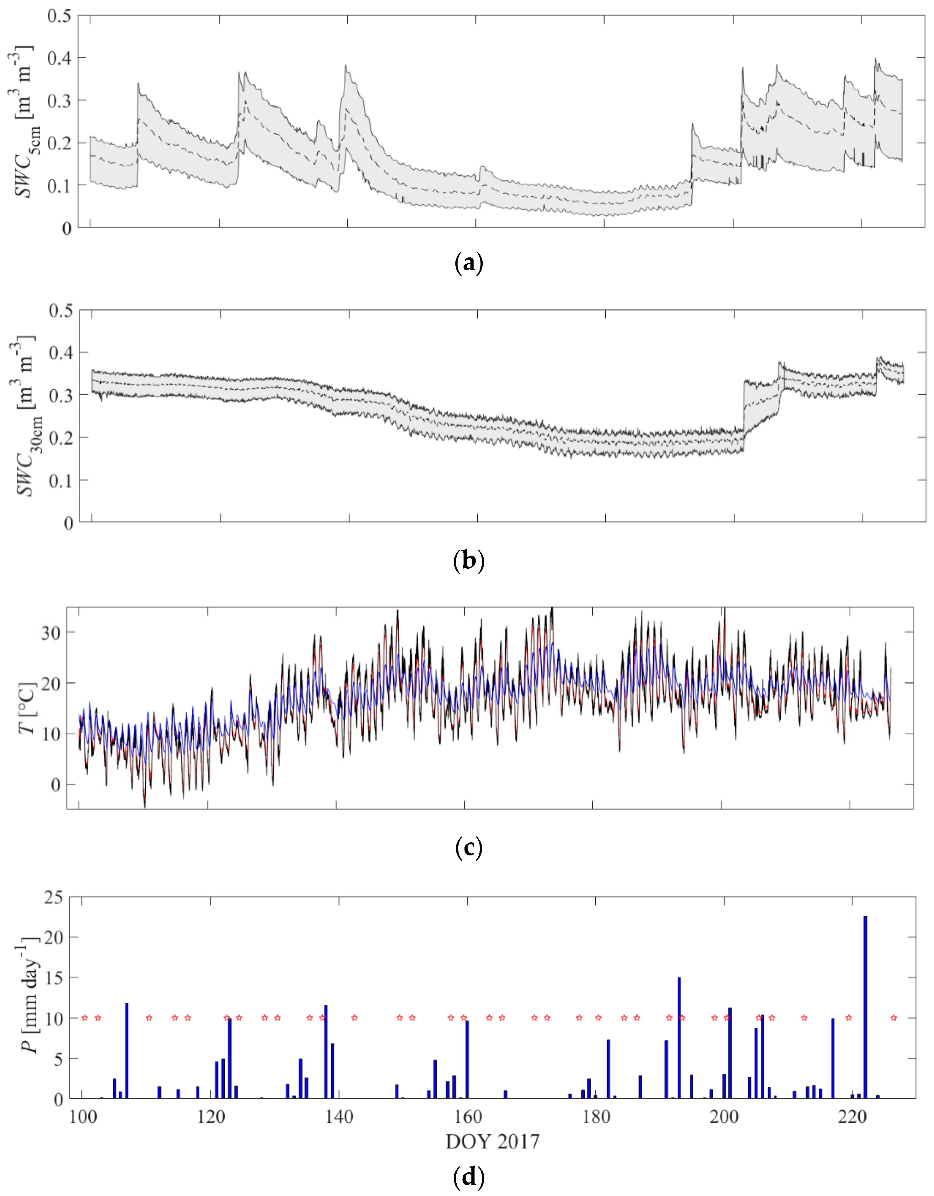
4.1. Ground Truth Measurements

Figure 3a,b shows the volumetric soil water content (SWC) measured at 5 and 30 cm depth, respectively. The black dashed line in Figure 3a represents the temporal evolution of the mean value of all 5TM/TE (5 cm) measurements from the two sampling locations, while the black dashed line in Figure 3b represents the temporal evolution of the mean value of all TDR (30 cm) measurements from the trench in the non-gridded plot. Additionally, the 75% quintile (grey shaded area) is depicted. As expected, higher values of SWC can be observed at 30 cm depth in comparison to 5 cm depth with a mean value of 0.27 m³ m⁻³ at 30 cm depth and 0.16 m³ m⁻³ at 5 cm depth over the entire growing season. In general, the time course of the volumetric soil water content at 5 cm depth can be separated into three major phases. In the first phase, the time period up to DOY 140 is characterized by wetter soil conditions caused by repeated rainfall and low evapotranspiration due to colder weather conditions and low plant stand. In the second phase, the SWC drops down between DOY 140 and DOY 193 due to low rainfall and high evapotranspiration caused by higher air temperatures and a developing crop stand. In the last phase, beyond DOY 193, SWC increases again due to higher rainfall.

The vegetation, air, and soil temperature are depicted in Figure 3c. The vegetation canopy temperature (T_C) and air temperature (T_A) show strong fluctuations, with a mean value of 16.2 °C and 16.1 °C and a STD of 7.1 and 6.3 °C, respectively. In comparison, the soil temperature (T_S) remains more stable over time with a slightly higher mean of 17.3 °C and a STD of 4.6 °C. In this sense, there is no significant difference between the T_C and T_A, and also, the difference between the T_C and T_S is negligible (about 1 °C).

Finally, the daily precipitation (P) is shown in Figure 3d, which is an important influencing factor on the measured T_B and also a factor controlling the plant growth. As can be seen, only a few rain events occur during the period between DOY 100 and 180, while more frequent rainfalls can be observed after DOY 180. The cumulative precipitation over the experimental time course was 210 mm.

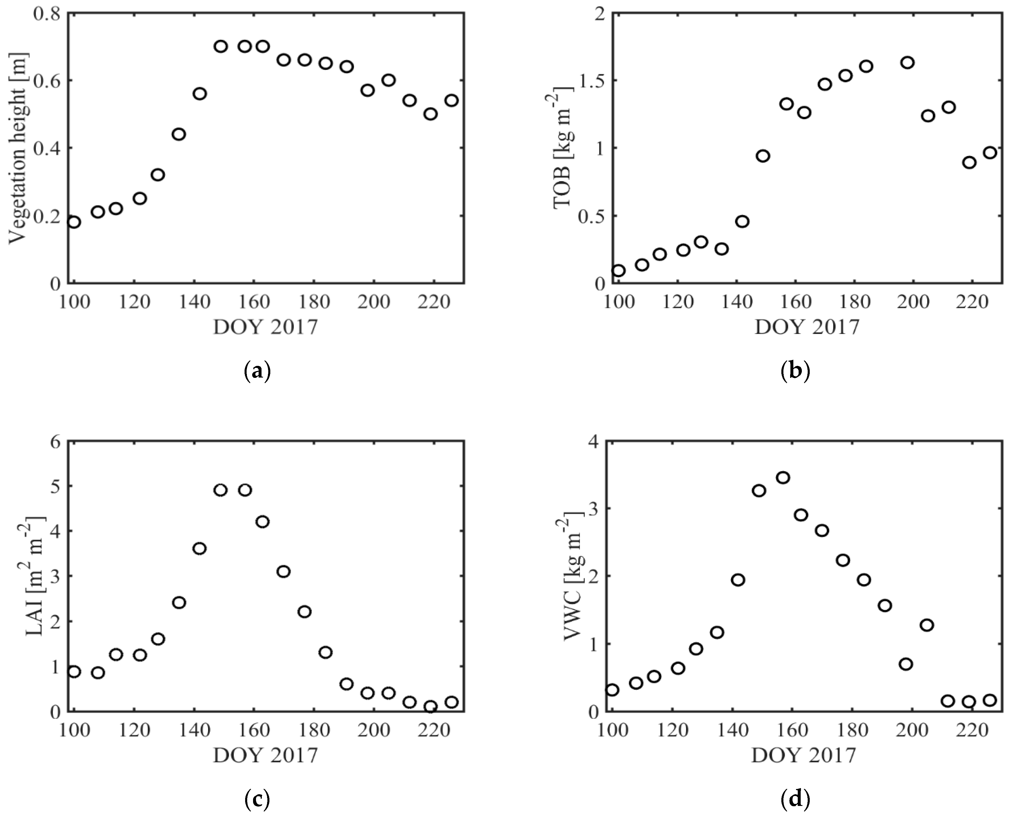
Figure 4a–d depicts all vegetation properties which were measured weekly in situ or in the laboratory over the entire growing season. Additionally,

Table 2. Overview of growth stages of the winter wheat between 10th of April (DOY 100) and 14th of August 2017 (DOY 226) and their corresponding BBCH scale values.

DOY 2017	Growth Stages	BBCH
100	Tillering	26
108–122	Stable stem elongation	30
128–142	Further stem elongation (increased plant growth rate)	35
142–149	50% of inflorescence visible	55
157	Beginning of flowering	61
163	Grain development started	71
180	Grain fully developed and start of ripening process	77 and 83–89
190–226	Early senescence to late senescence	92–99

gives an overview of the growth stages of the winter wheat and their corresponding BBCH scale values. The vegetation height, the leaf area index (LAI), and the vegetation water content (VWC) increased during the first 50 days of the growing season, reaching a maximum value of about 0.7 m, 5 m² m⁻², and 3.5 kg m⁻³, respectively, and started to decline after DOY 160. The total of aboveground biomass (TOB) reached a maximum value of about 1.5 kg m⁻² around 40 days later on DOY 190. These different developments correspond to specific growing stages. The field campaign started during the tillering stage (BBCH 26) at DOY 100, followed by a stable stem elongation period (BBCH 30) with no significant change between DOY 108 and 122. After the air temperature started to increase and stayed above 10 °C, the growing stage increased to a BBCH scale value of 35 between DOY 128 and 142, which corresponds to a further stem elongation. Between DOY 142 and 149, the plant growth rate of the winter wheat canopy increased exponentially, and about 50% of the inflorescence was visible at the end of this period (BBCH 55). The whole timeframe between DOY 120 and 150 is characterized by a strong increase in the measured vegetation properties. With the beginning of the flowering (BBCH 61) at DOY 157, a clear decline of the LAI and VWC was detectable, and the vegetation height also began to decrease. The grain development (BBCH 71) started a few days later, around DOY 163, and a further decline of the measured vegetation properties was observable (strongest for the VWC and LAI, not yet for TOB). The grain was fully developed (BBCH 77) at around DOY 180 and had already started with the ripening process (BBCH 83 until 89) in some parts of the stand. Around DOY 190, the early senescence phase started (BBCH 92), after which the TOB also began to decrease due to vegetation loss (mainly leaves and grains). DOY 226 represents the totally senescent vegetation (BBCH 99), where the LAI and VWC dropped to their minimum values, but the vegetation height and TOB remained relatively constant, as the vegetation was not harvested before the end of this experiment.

Finally, whether the weather and soil moisture conditions were sufficient to support plant growth over the entire growing season was investigated. As can be seen from Figure 3 and Figure 4, the temporal evolution of the measured vegetation properties and SWC do not indicate any clear water stress nor stagnation in growth and biomass gain during the whole growing season.

4.2. Radiometer Data

4.2.1. Radiometer Measurements over the Gridded Plot

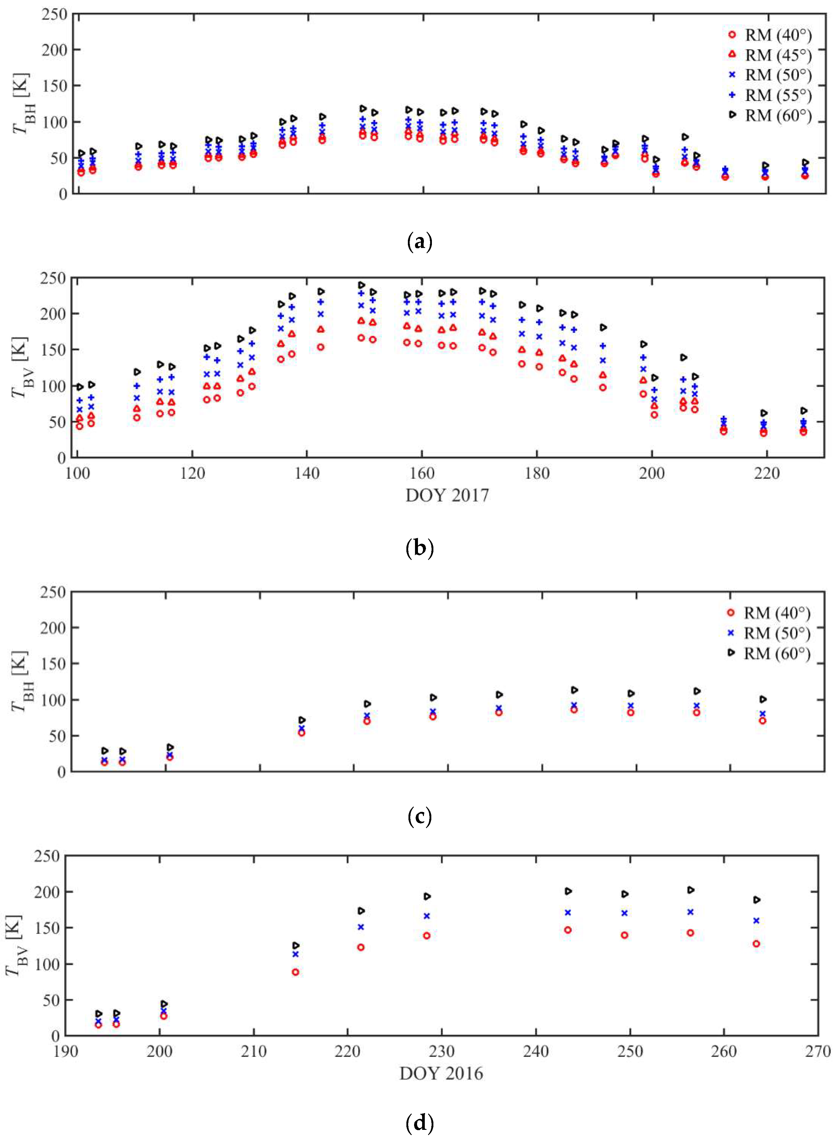
Figure 5a,b depicts the L-band brightness temperatures (T_B) at H and V polarization observed over the gridded plot within the winter wheat stand. For both polarizations, a clear seasonal trend is detectable, which can be generally separated into three phases. In the first phase, T_B increased at the beginning of the growing season, reaching a first peak at DOY 140. This increase in T_B corresponds well to the increase of the above-mentioned vegetation properties (see also Section 4.4). In the second phase, between DOY 145 and DOY 175, T_B values were relatively stable over time. Within this period, also, no significant changes in the vegetation layer were detectable. During the third phase, starting after DOY 175 and continuing until the end of the growing season (DOY 226), T_B significantly decreased. This decrease in T_B is mainly related to the reduction in VWC and LAI (due to leaf loss), whereby the vegetation height and TOB remained constant during the same period.

Secondly, T_BV measurements show a higher temporal variability with general higher values over the entire growing period, but also a larger increase during the crop development compared to T_BH. This observation can be explained by the stronger vertical orientation of the wheat canopy, leading to a higher emission contribution in the V polarization.

Furthermore, a clear angle dependency with highest T_B values at 60° angle is detectable, whereby the angular dependency is much more pronounced for T_BV compared to T_BH. The lower variability over time of T_BH can be also confirmed by the lower STD values. For T_BH, the mean values are 52.6 K (40°), 56.7 K (45°), 62.2 K (50°), 70 K (55°), and 82.6 K (60°), with a STD ranging between 18.4 K (40°) and 23.6 K (60°), while for T_BV, the mean values are 108.4 K (40°), 124.1 K (45°), 138.1 K (50°), 153.8 K (55°), and 172.6 K (60°), with a STD of 53 K (same for all angles). Additionally, the magnitude of the angular dependency does not change much between DOY 100 and DOY 200 for either polarization. After DOY 200, the angular dependency disappears at a stage when the vegetation begins senescence, which confirms that this dependency is mainly caused by changes in VWC and LAI. In summary, these results show that the changes in T_B are mainly driven by the vegetation status. This proves that our setup is adequate to detect significant contrasts in T_B, and therefore, different vegetation canopy states within the radiometer footprints.

To confirm these general findings, we included data from a short experiment performed with white mustard (Sinapis alba L.) during summer 2016 using the same setup as for the winter wheat experiment in 2017. Unfortunately, measurements for white mustard were stopped before the plant reached the senescent stage, and therefore, VWC and LAI reached only a maximum value and did not decline. The T_B measured at H and V polarization is shown in Figure 5c,d. As can be seen, the white mustard vegetation shows the same characteristics in the T_B evolution over time as the winter wheat canopy. Compared to winter wheat, the increase and angular dependency is less pronounced in V polarization, which can be explained by the less vertically dominant structure of mustard plants and lower VWC. Additionally, the difference between T_BH and T_BV is lower in magnitude, which is confirmed by the mean values and the STD. For T_BH, mean values are 58.6 K (40°), 65.4 K (50°), and 81.3 K (60°), while the STD values are 29.4 K (40°), 31.6 K (50°), and 35.1 K (60°). On the other hand, for T_BV, the mean values are 96.2 K (40°), 117.7 K (50°), and 138.6 K (60°), while the STD values are 55.7 K (40°), 66.2 K (50°), and 74.9 K (60°).

Finally, the brightness temperature at the beginning of the mustard experiment, i.e., with the reflecting grid on the bare soil, was slightly higher than the sky brightness temperature (T_B-SKY ~ 5 K), with a mean value of 12.4 K (DOY 193) and 12.7 K (DOY 195) at H polarization and 14.8 K (DOY 193) and 16 K (DOY 195) at V polarization at a 40° incidence angle. This difference between the measured T_B above the reflecting grid and the T_B-SKY results mainly from the areas not covered by the grid, as described in Jonard et al. [28]. However, it can be assumed that the radiance originating from the surrounding area remains stable during the experiment, allowing us to not correct for this difference. Nevertheless, using higher incidence angles leads to an increase in the contribution of the surrounding area radiance to the measured T_B.

4.2.2. Radiometer Measurements over the Non-Gridded Plot

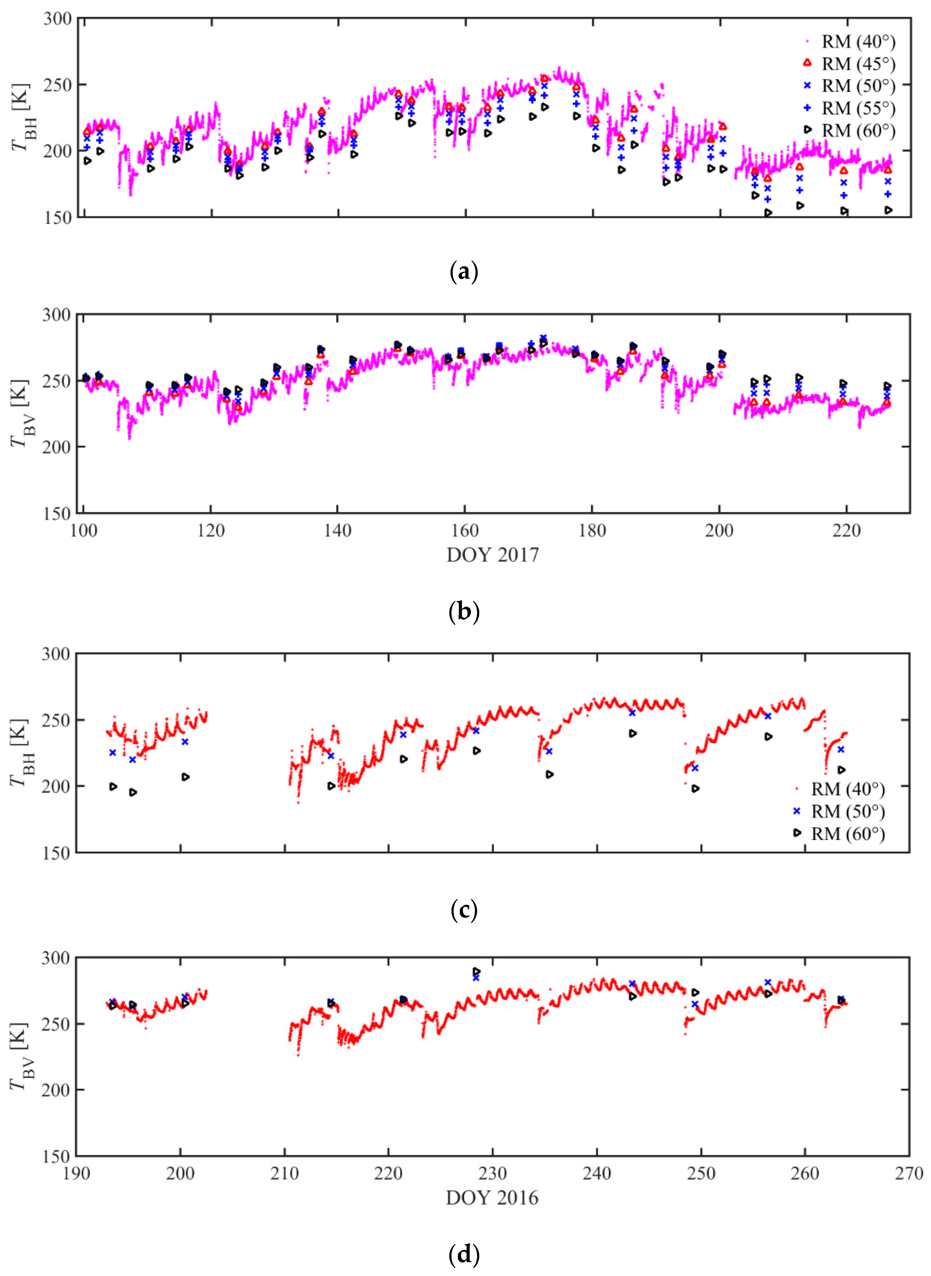
Figure 6a,b shows the T_B measurements at H and V polarization above the non-gridded plot within the winter wheat stand. Again, both polarizations indicate comparable time courses over the growing season with relatively stable T_B between DOY 100 and DOY 140 with values of about 200 K (T_BH) and 250 K (T_BV), respectively, followed by an increase in T_B up to 250 K for T_BH and 270 K for T_BV between DOY 140 and 180. Furthermore, this general pattern is also in good agreement with the changes in the vegetation properties (mainly the VWC and LAI) (see Figure 4a,b), whereby the more noisy character of the data is an indication of changes in the soil moisture due to precipitation events (see Figure 3a,d). As expected, T_BV was systematically higher compared to T_BH during the entire growing period with mean values of 215.0 K (40°), 214.7 K (45°), 209.7 K (50°), 203.7 K (55°), and 195.4 K (60°) for T_BH and 247.5 K (40°), 255.9 K (45°), 259.3 K (50°), and 261.7 K (55°), and 261.5 K (60°) for T_BV. Concerning the temporal evolution, T_BH can be characterized by a stronger temporal variability compared to T_BV, with a STD of about 21 K for T_BH and about 14 K for T_BV for all incidence angles. Additionally, after DOY 180 until the end of the growing season, the T_BV only decreased by 30 K, to values around 240 K, while T_BH decreased much more significantly, by about 70 K, down to values around 150 K for the 60° angle, and by about 50 K, down to values around 190 K for the 40° angle. This strong decrease of T_BH is governed by two opposing factors, namely, the linear decrease of VWC and LAI (i.e., decrease of vegetation layer emission), and the increase of SWC from mean values around 0.1 m³ m⁻³ to SWC of about 0.3 m³ m⁻³ at 5 cm depth. This change in soil moisture is associated with a decrease of soil surface layer emission. Therefore, the impact of the surface soil moisture on T_B was dominant compared to the impact of the changes in VWC or LAI during the senescent phase of the winter wheat canopy.

Focusing on the angular dependency of the measured T_B, T_BH has in general a stronger angular dependency compared to T_BV. Additionally, T_BH shows a decrease with increasing incidence angle (T_B-40° > T_B-60°), which is in contrast to the observations over the gridded plot, where T_BH increases with increasing angle. It can also be seen that the sensitivity of T_BH with respect to the measurement angle increases after DOY 180 and is strongest when the vegetation layer reaches the senescence stage. This increase of the angular dependency may be explained by the larger influence of the soil layer emission (with relatively smooth surface) on the measured T_B at H polarization [39]. In comparison, the angular dependency of T_BV (increasing T_BV with increasing incidence angle) is much weaker over the growing season, showing the strongest dependency after DOY 200.

Again, the data collected for the winter wheat were compared to the mustard experiment data. As can be seen, T_B data collected for the mustard stand shows similar patterns with a stronger temporal variation and angular dependency for T_BH (Figure 6c,d). However, both T_BH and T_BV are, in general, higher and also more stable over the growing season of the mustard vegetation. The main reason for this can be found in the generally lower SWC at 5 cm depth (mean value of 0.1 m³ m⁻³) with lower temporal fluctuations (STD of 0.04 m³ m⁻³) during the mustard experiment and the lower influence of the vegetation layer changes. Here, it has to be noted that the precipitation events were also less frequent with a total precipitation of only 73 mm over the entire mustard growing season. The angular dependency of T_BH becomes smaller at the end of the mustard experiment, corresponding to the highest VWC and LAI values (~3 kg m⁻³ and 2 m² m⁻², respectively), and therefore, to a lower sensitivity of T_B to the soil layer emission.

To underline these observations, we again calculated the mean values, which are 241.5 K (40°), 232.3 K (50°), and 213.1 K (60°), and the STD values, which are 15.7 K (40°), 13.3 K (50°), and 15.7 K (60°) for T_BH; while for T_BV, the mean values are 264.5 K (40°), 271.1 (50°), and 269.7 K (60°) and the STD values are 10.4 K (40°), 7.6 K (50°), and 7.6 K (60°).

4.3. Vegetation Optical Depth

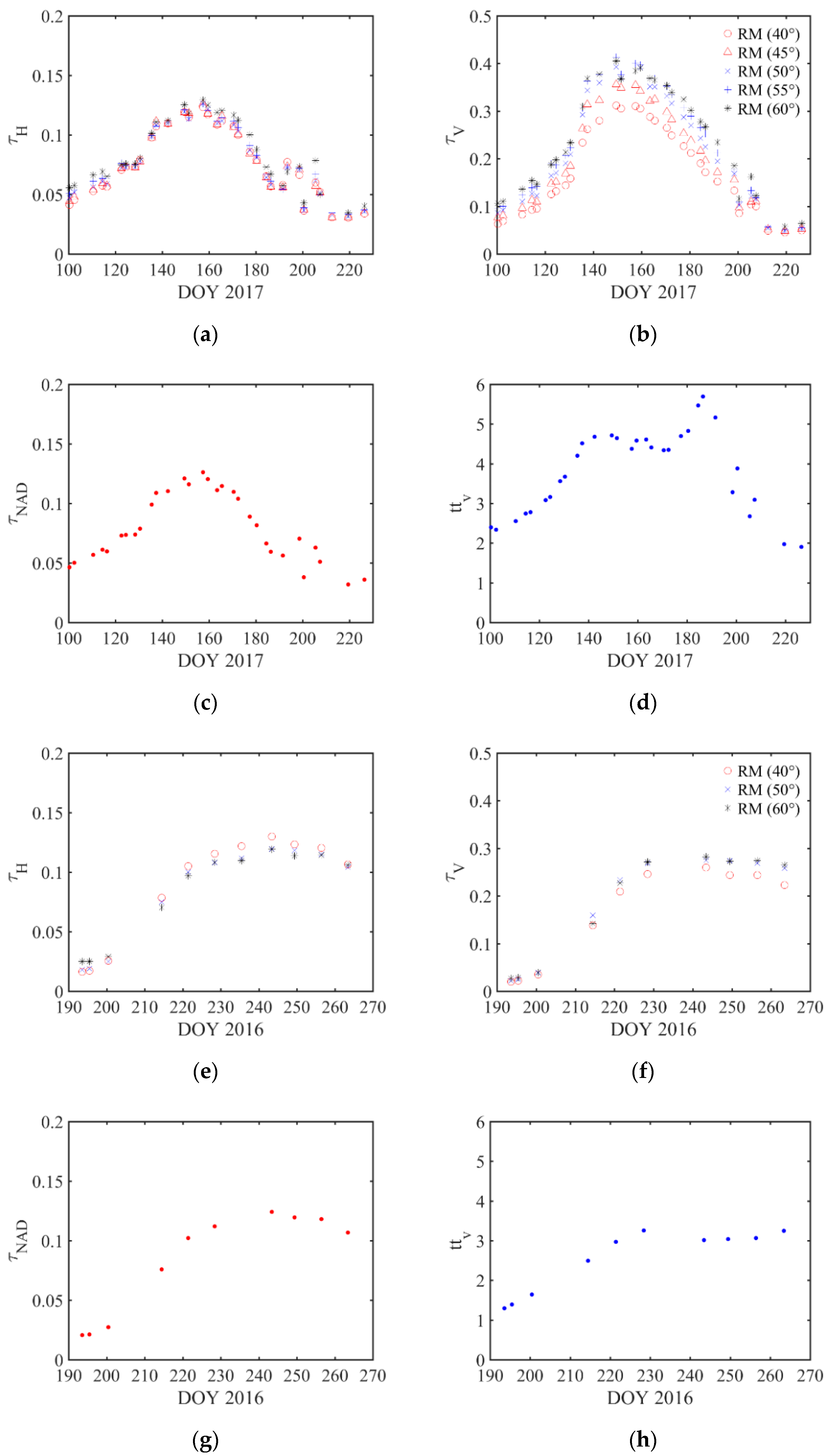
In this section, the results of the retrieval of the vegetation optical depth (τ_p) from the T_B data collected over the gridded plot using the τ-ω model are presented. Figure 7 illustrates the temporal evolution of the retrieved τ_p values using the single-angle (a,b and e,f) and the multi-angle retrieval approach (c,d and g,h) at H and V polarization for the winter wheat and the white mustard vegetation, respectively.

For the wheat vegetation, the results of the τ retrieval using the single-angle approach show a pronounced temporal evolution over the growing season, with generally lower values at H (Figure 7a) compared to V polarization (Figure 7b). The lowest τ_p values can be observed at the beginning of the growing season (tillering stages) and at the end of the experiment during the senescence stages, while the highest values can be observed around DOY 150 to 160, corresponding to the period at the end of flowering. The mean and STD of τ_H is 0.09 and 0.03, respectively, for all different angles. The mean values of τ_V on the other hand increase with increasing incidence angle with values of 0.2 (40°), 0.23 (45°), 0.26 (50°), 0.28 (55°), and 0.31 (60°). The STD is also much higher compared to that for τ_H, with values of 0.11 (40°), 0.14 (45°), 0.15 (50°), 0.15 (55°) and 0.15 (60°). These data show a clear angular dependency of τ at V polarization. The magnitude of the angular dependency increases between DOY 140 and 160, meaning that the highest angular dependency occurred for a fully developed vegetation cover (around DOY 160), which was characterized by a maximum VWC and LAI and a maximum stem elongation. The lowest angular dependency is observed for a fully senescent vegetation canopy (after DOY 200).

For the multi-angle retrieval approach, τ was not estimated for a specific incidence angle as the T_B data from all angles were used simultaneously in the retrieval. Therefore, τ at nadir angle (τ_NAD), as well as the structural parameter tt_p used to account for polarization dependency on τ, were obtained using Equation (4). In this study, tt_H (structural parameter at H polarization) was assumed to be equal to 1, as the winter wheat has a dominant vertical structure. This was also confirmed by the results of the single-angle retrieval approach (see above), showing no significant differences between the τ retrievals at different incidence angles. As expected, using the assumption of tt_H equal 1, the temporal evolution of τ_NAD is very similar to the one observed for τ_H retrieved by the single-angle approach. Concerning the temporal evolution of tt_V, the values are the highest during the main growing phase of the vegetation (between DOY 130 and 180), showing a clear peak around DOY 193 due to wetting of the vegetation during a large rain event and lowest at the beginning and the end of the growing season (Figure 7c,d). The mean and STD of tt_V are 3.82 and 1.05, respectively.

Concerning the retrievals of τ_H and τ_V of the mustard vegetation using the single-angle approach, there is also a clear polarization and temporal dependency observable with higher τ values in the V polarization, but less strong in magnitude compared to the winter wheat stand. Furthermore, the angular dependency of τ_V is lower, which indicates less anisotropic conditions of the mustard vegetation at L-band (Figure 7e,f). The mean values and STD of τ_H are 0.08 and 0.18 (same for all angles), respectively, while the mean values and STD of τ_V are 0.04 and 0.11 (also same for all angles), respectively. 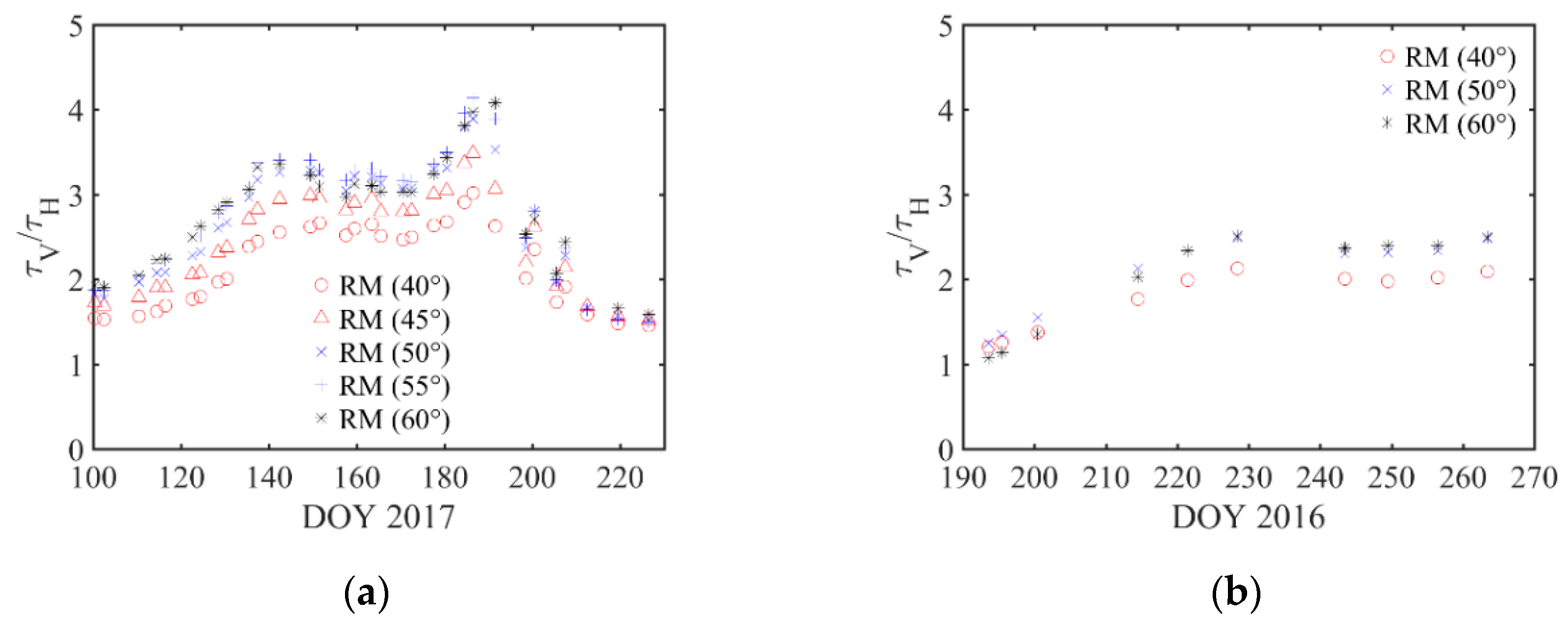The lower anisotropy in the vertical polarization for the mustard compared to the winter wheat can be also seen in the retrieved tt_V parameter, where the mean and STD are 2.54 and 0.80, respectively (Figure 7g,h). Finally, the ratio between the τ_H and τ_V was also calculated and is depicted in Figure 8a,b for wheat and mustard vegetation, respectively. It can be seen that for the wheat, the ratio varies between 2 and 4, with a very stable period during the main growing season between DOY 130 and 190 and a peak around DOY 193, which corresponds again to the wetting of the vegetation after a strong precipitation event (about 15 mm). During the tillering and the senescence stages, the difference between the H and V polarization is reduced (values around 2), which suggests more isotropic conditions. The ratio between the τ_H and τ_V for the mustard vegetation varied between 1 at the beginning of the growing season (DOY 193 to 200) and 2.5 at the end of the experiment campaign. These results confirm again that the mustard canopy is more isotropic compared to the wheat vegetation (i.e., the τ parameter is less dependent on the measurement angle and polarization). It has also to be noted that the mustard experimental campaign started with bare soil conditions, while the winter wheat plants already had a height of 20 cm at the beginning of the measurement campaign (see Section 4.1). This can explain the higher τ values for winter wheat during the first measurement days.

4.4. Relationship between Vegetation Optical Depth and In Situ Measured Vegetation Properties

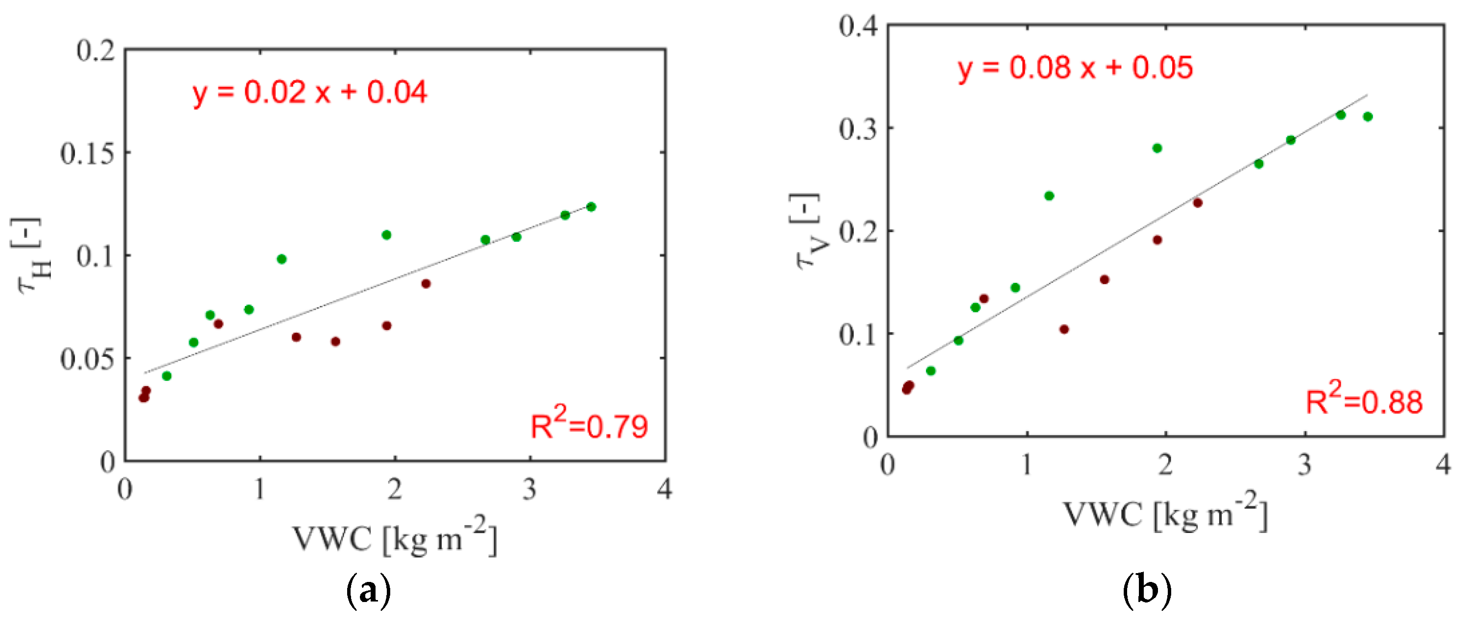
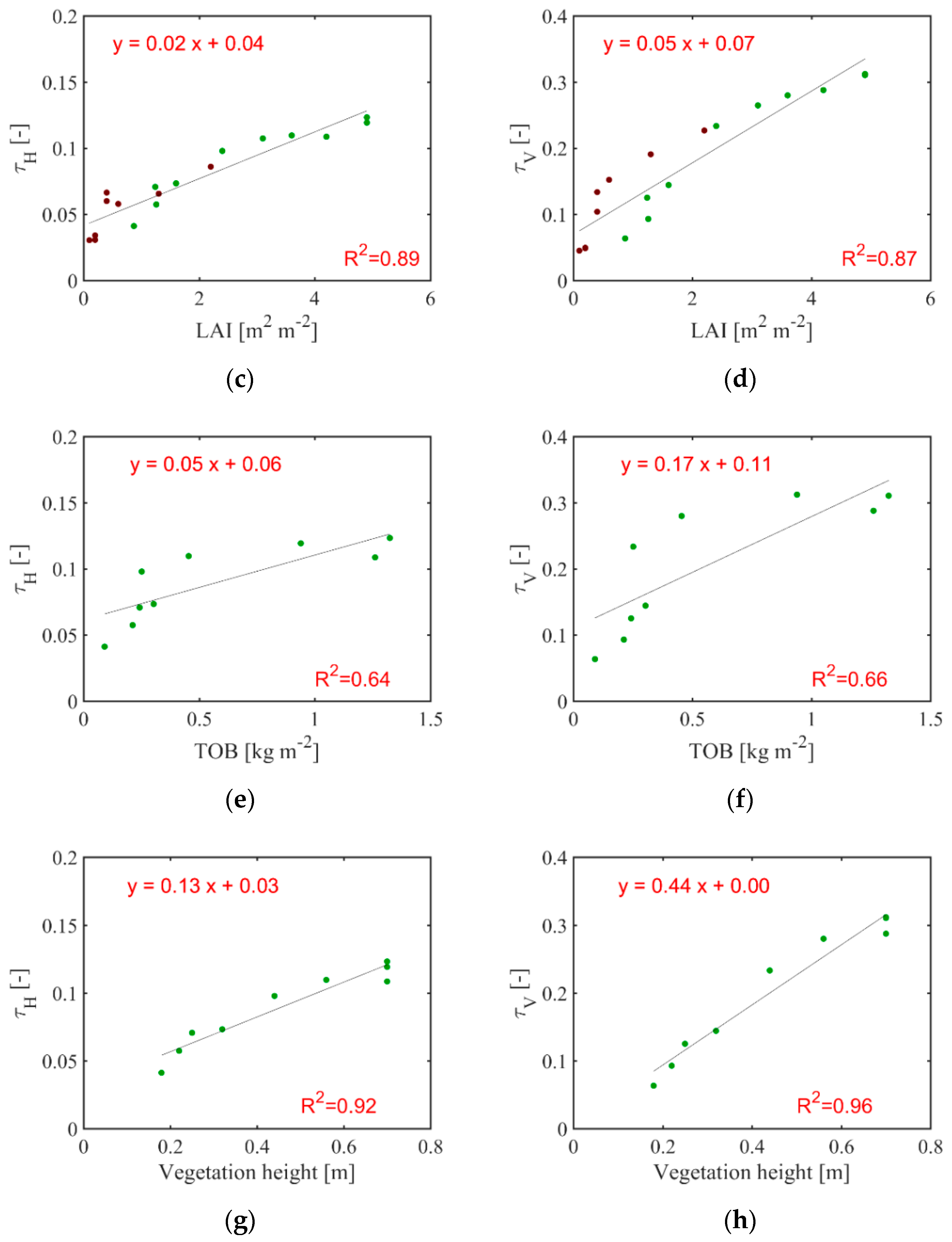
In this section, the relationships between the retrieved vegetation optical depth and in situ measured vegetation properties (VWC, LAI, TOB, and vegetation height) are analyzed based on linear regressions. For that, the τ values retrieved from the 40° T_B data measured over the gridded plot (see Figure 7a,b) were used. The results of these regressions are shown in Figure 9a–h. As the in situ vegetation parameters were only measured at 19 observation dates (see Figure 4a–d), the corresponding τ_p values were only selected for those days, reducing the number of observation pairs to n = 18. Additionally, for the TOB and vegetation height, as we are only interested in the plant growth stages (i.e., when plants grow and vegetation water content rises) for the relationship between τ_p and these two parameters, only the first ten measurements were selected for the regression reducing the number of observation pairs to n = 9. Indeed, these two vegetation parameters do not show the same bell-shaped temporal evolution as τ, but mainly an increase for the early growing stages until DOY 150, and then constant values followed by a small reduction in the late growing stages (see Figure 4c,d).

Figure 9 shows the linear regressions between τ_p and the vegetation properties. The slope, intercept, and R² are also depicted on the plots. In general, high correlations between τ and the vegetation parameters are obtained with R² values ranging from 0.64 to 0.96. The lowest correlation is obtained between τ_p and TOB with R² values of 0.64 and 0.66 for τ_H and τ_V, respectively, while the best correlation is observed between τ_p and the vegetation height with R² values of 0.94 and 0.96 for τ_H and τ_V, respectively. The correlation between τ_V and VWC and the one between τ_V and LAI show quite similar R² values, i.e., 0.88 and 0.87, respectively. On the contrary, the correlation between τ_H and VWC is lower, with a R² of 0.79, compared to that between τ_H and LAI, with a R² of 0.89. The lower correlation between τ_p and TOB can partly be explained by the fact that the maximum value of TOB (DOY 190) is reached later than the maximum value of τ_p (DOY 150) (see Figure 4 and Figure 7a,b), while the maximum values of the three other vegetation properties are reached at nearly the same time as τ_p.

The slope and the intercept of the regression lines are always positive. The slope is systematically much lower than 1, and the intercept is generally close to 0 with highest values for the TOB–τ_p relationship and lowest values for the vegetation height–τ_p relationship. The slope values for the VWC–τ_p and LAI–τ_p relationships correspond well to the ones reported by Wigneron et al. [13] for a wheat vegetation stand, where slope values of 0.08 and 0.03 were found for the VWC–τ_p and LAI–τ_p relationships, respectively. However, Wigneron et al. [13] found negative values for the intercepts, i.e., −0.02 and −0.01 for the VWC–τ_p and LAI–τ_p relationships, respectively. It has to be noted that in the study of Wigneron et al. [13], vegetation optical depth at nadir angle (τ_NAD) was considered instead of τ_p.

In a next step, the so-called b parameter was analyzed, which is classically used to relate the VWC or LAI to the τ_p parameter using:

$${\mathsf{\tau }}_p=b_{\mathrm{VWC}}VWC,$$

(6)

$${\mathsf{\tau }}_p=b_{\mathrm{LAI}}LAI.$$

(7)

Equation (6) has been found to be valid in several studies (e.g., [40]). The b_VWC parameter is often set to 0.12 for agricultural crops, as reported by Wigneron et al. [13]. In the current Level 3 SMAP algorithm (SMAP SCA), Equation (6) is used to estimate the τ parameter based on information from ancillary data of VWC extracted from MODIS NDVI data and b parameter values derived from a look up table for different land-cover classes [41]. However, the LAI can also be used as a proxy for the estimation of τ (Equation (7)), as LAI is classically retrieved on a global scale [13]. 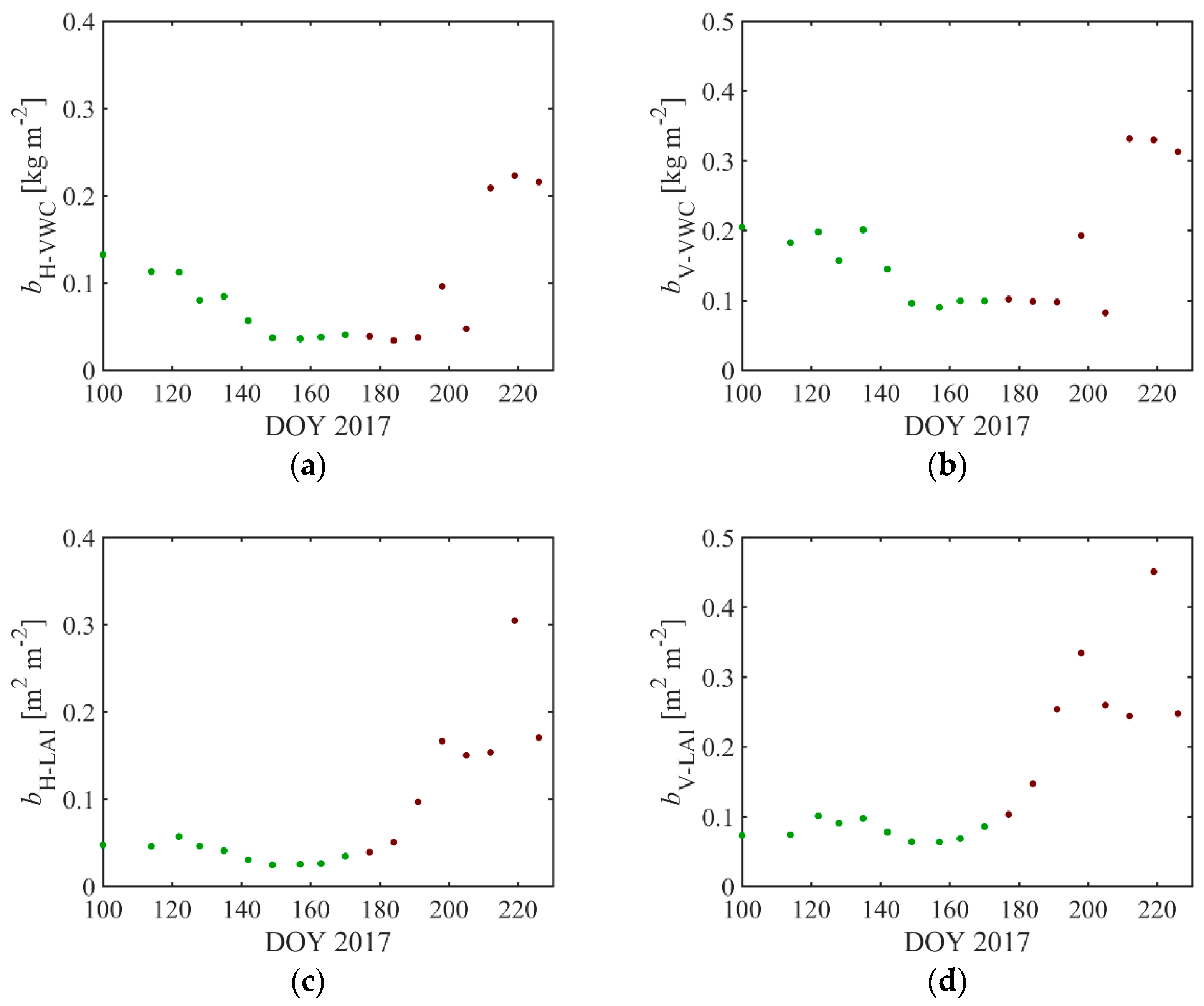Figure 10 depicts the b parameters estimated from the 40° angle τ values derived from single-angle approach. The b_VWC parameter at H and V polarization shows a clear dependency on the growing stages with decreasing values between DOY 100 and 150, relatively stable values between DOY 150 and 200, and increasing values after DOY 200 (Figure 10a,b). The first period corresponds to strong changes in the vegetation structure (stem elongation) and the VWC, followed by a linear decrease of the VWC in the second period, with no significant changes of the vegetation structure. During the third period, a further decline of the VWC was measured as the plants became senescent. Additionally, the vegetation structure changed, whereby the wheat heads and stems were stronger orientated towards the soil surface leading to a decrease of the vegetation height and also a decrease in TOB due to a loss of leaves. The b_H-VWC parameter is, in general lower compared to b_V-VWC with a mean value of 0.09 in comparison to 0.17 for b_V-VWC. Figure 10c,d shows that the b_LAI parameter is less sensitive to vegetation growing stages, with relatively constant values of around 0.05 for b_H-LAI and 0.1 for b_V-LAI between DOY 100 and 190. After this, b_LAI increases strongly for both polarizations as the vegetation structure changes significantly during senescence. Again, the b_LAI parameter is, in general, lower at H polarization, with a mean value of 0.08, compared to 0.16 for the V polarization.

In conclusion, the results show that the b parameters are only constant during the middle of the growing season, i.e., when the wheat vegetation was fully developed for the VWC approach (Equation (6)), whereby for the LAI-based approach (Equation (7)), the b parameters can be assumed to be constant for the entire growing season, except for the senescence stages. Finally, the b parameter is, in general, higher at V polarization, which could be explained by the fact that the vegetation was predominantly oriented in the vertical direction [23]. These results are consistent with the findings of Zakharova et al. [42], who observed a similar evolution of a polarization-independent b_VWC parameter for low vegetation canopies (i.e., grassland, wheat and irrigated maize). They showed a clear decrease of the b_VWC parameter during the vegetation growing phase, with b values of 0.15 during spring and values around 0.05 during summer, when the vegetation was fully grown.

4.5. Volumetric Soil Water Content

Volumetric soil water content (SWC) was retrieved from T_B observations performed over the non-gridded area using the different retrieval schemes (1-P, 2.1-P, 2.2-P, and 3-P) described in Section 3.2 (see Table 1). A summary of the comparison between the measured and modeled SWC for the different retrieval schemes is depicted in

Table 3. Summary of the comparison between the measured and modeled volumetric soil water content (SWC) (m³ m⁻³) for the different retrieval schemes. Unbiased root-mean-square-error (ubRMSE), bias, and coefficient of determination (R²) values are shown.

	Single-Angle Approach			Multi-Angle Approach
Retrieval Schemes	ubRMSE	bias	R2	ubRMSE	bias	R2
1-P	0.047	0.013	0.57	0.047	−0.002	0.58
2.1-P	0.054	−0.044	0.42	0.055	−0.056	0.40
2.2-P	0.062	0.124	0.43	0.050	0.089	0.68
3-P	-	-	-	0.050	0.089	0.68

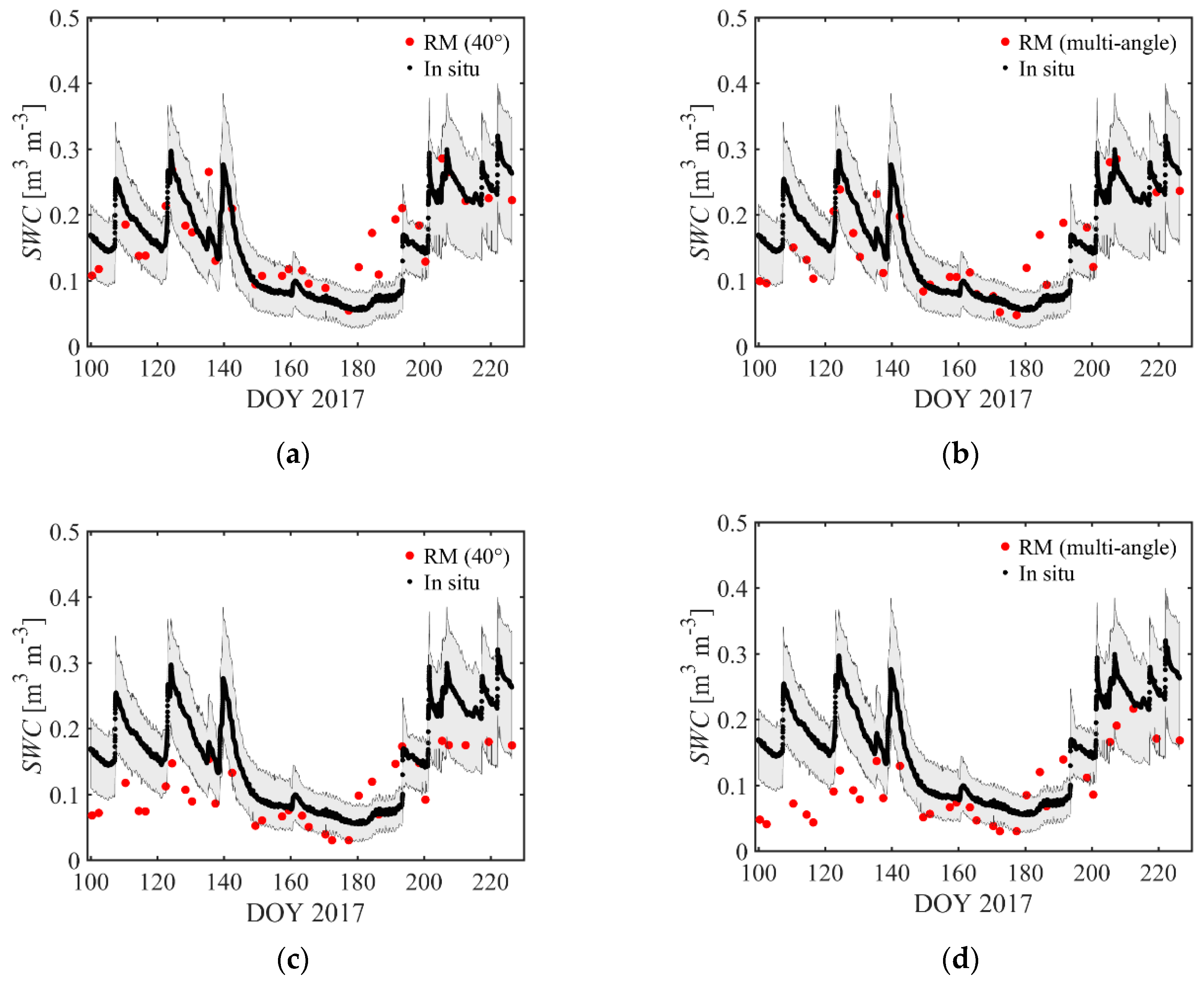
. The unbiased root-mean-square-error (ubRMSE) [43], bias, and coefficient of determination (R²) values are shown for the single- and multi-angle approach, respectively. The results based on the 1-P retrieval scheme (estimation of SWC alone) are shown in Figure 11a,b for the single- (40° incidence angle) and multi-angle (from 40° to 60° incidence angle) approach, respectively. The estimated SWC values are in good agreement with the in situ measurements as confirmed by the ubRMSE and bias values of 0.047 m³ m⁻³ and 0.013 m³ m⁻³ for the single-angle approach, and 0.047 m³ m⁻³ and −0.002 m³ m⁻³ for the multi-angle approach. In addition, the R² of 0.57 (single-angle) and 0.58 (multi-angle) also indicate a good agreement between the data sets.

The SWC values retrieved based on the 2.1-P retrieval scheme (estimation of SWC and ω) are illustrated in Figure 11c,d and indicate, in general, a relatively poor agreement between the measured and modeled SWC with a R² of 0.42 and 0.40 for the single- and multi-angle approach, respectively. The bias is significantly larger compared to the 1-P retrieval scheme with a value of −0.044 m³ m⁻³ for the single-angle approach and −0.056 m³ m⁻³ for the multi-angle approach. This indicates a large underestimation of the retrieved SWC in comparison to the in situ data. Also, the ubRMSE with values of 0.054 m³ m⁻³ and 0.055 m³ m⁻³ for the single- and multi-angle approach, respectively, shows slightly higher values in comparison to the 1-P retrieval scheme. 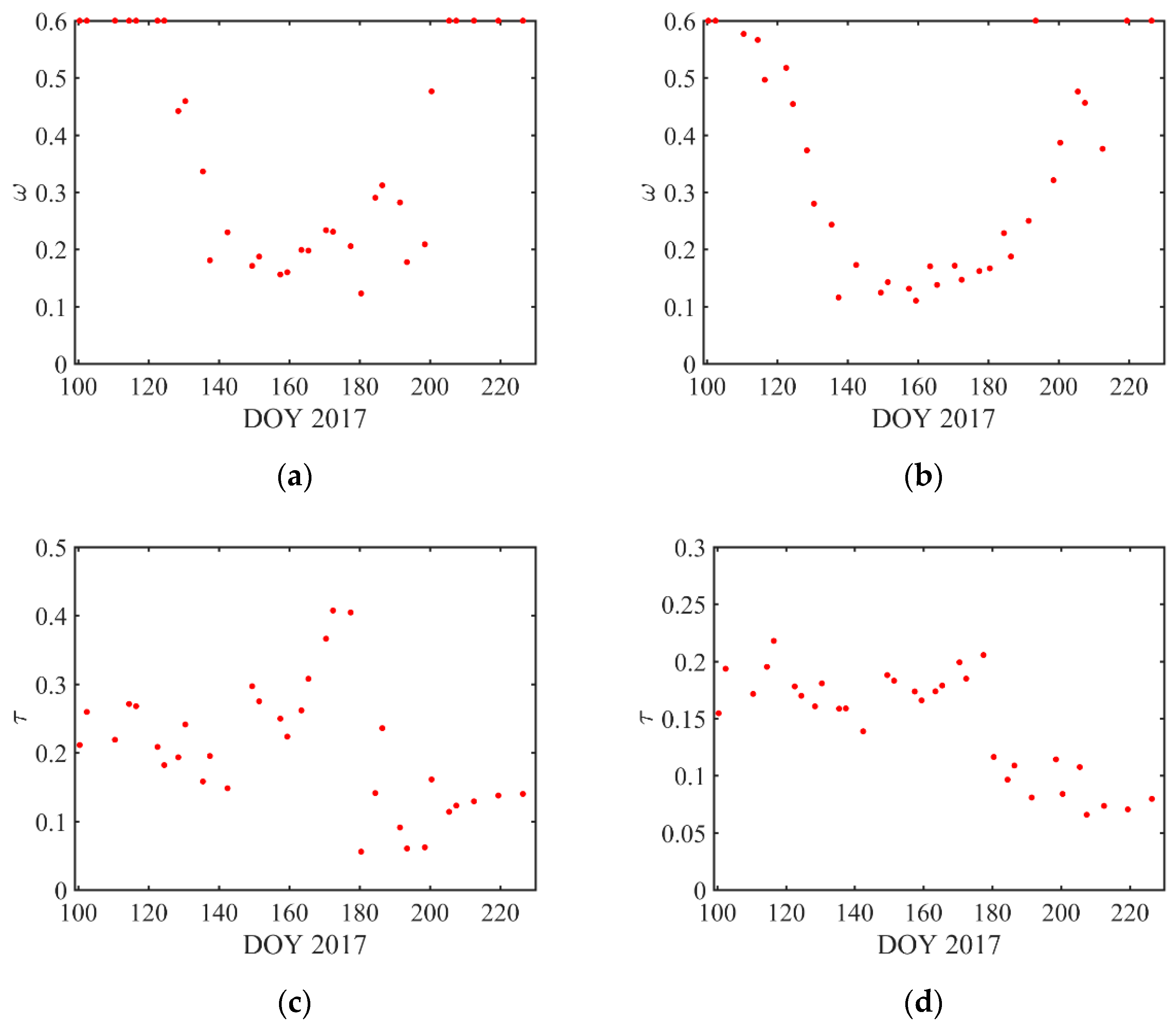As can be seen in Figure 12a,b, the retrieved ω values are very high at the beginning and at the end of the growing season, decrease with growing vegetation (DOY 120 till 140), then show relatively constant values around 0.1–0.2 when the vegetation is fully grown (DOY 140 till 180), and finally increase when the vegetation becomes senescent (DOY 180 till 210). These results clearly indicate that the simultaneous retrieval of SWC and ω fails to obtain ω correctly. Indeed, values of ω at the beginning and at the end of the growing season were expected to be close to zero and, instead of a large decrease when the vegetation was fully grown, a small increase in ω was expected.

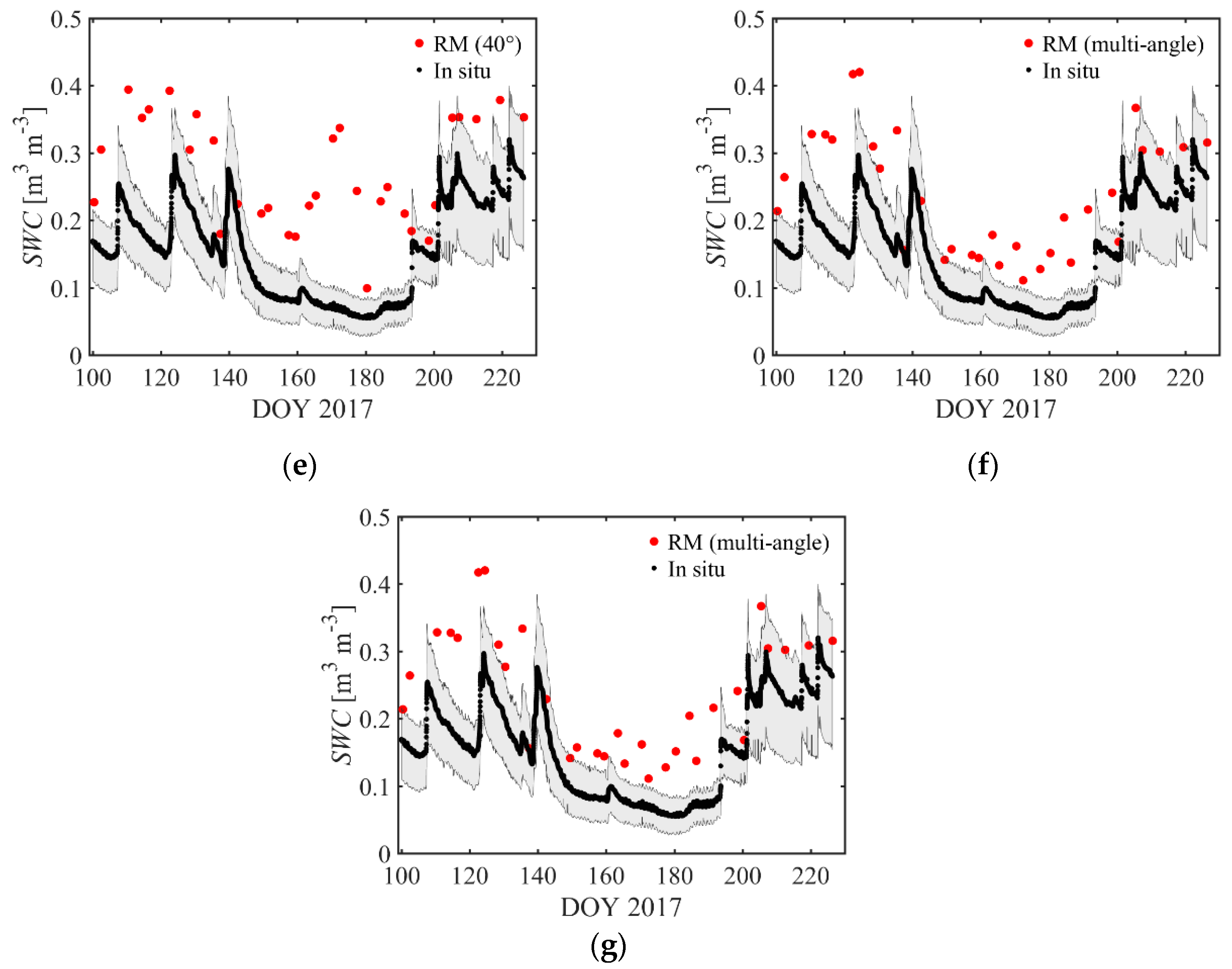
For the 2.2-P retrieval scheme (estimation of SWC and τ), SWC was retrieved without any prior information on the τ parameter. The 2.2-P retrieval scheme shows an ubRMSE and bias of 0.062 m³ m⁻³ and 0.124 m³ m⁻³, respectively, for the single-angle approach and 0.050 m³ m⁻³ and 0.089 m³ m⁻³, respectively, for the multi-angle approach (Figure 11e,f). Compared to the 1-P and 2.1-P retrieval schemes, the ubRMSE increases for the single-angle approach and slightly decreases for the multi-angle approach, and the bias of both approaches indicates a high overestimation of the modeled SWC values. Additionally, the R² of 0.43 for the single-angle approach indicates a relatively low correlation between modeled and measured SWC. On the contrary, the R² of 0.68 for the multi-angle approach indicates a good agreement. As shown in Figure 12c,d, the bell-shaped temporal evolution of τ retrieved from the gridded plot T_B data (see Figure 7a–d) could not be obtained for the single- and multi-angle approaches. However, for the single-angle approach, a clear increase in values around 0.4 between DOY 160 and DOY 180 is observed (Figure 12c), while for the multi-angle approach, the τ values are, in general, lower and show even lower temporal variations, with values around 0.1–0.2 (Figure 12d).

Finally, the results of the 3-P retrieval scheme (estimation of SWC, τ_NAD, and tt_V) using the multi-angle approach are depicted in Figure 11g. It has to be noted that the single-angle approach could not be used to retrieve three parameters, as not enough information is contained in the T_B measurements with only one incidence angle. The results show identical ubRMSE, bias, and R² values as the 2.2-P retrieval scheme based on the multi-angle approach. This can be explained by the fact that the 3-P approach did not succeed to retrieve the tt_V parameter correctly. Indeed, the retrieved ttv values are close to 1 for the whole growing period (results not shown), while tt_V is expected to be higher than 1 for wheat vegetation ([13] and see Figure 7d), and the retrieved τ_NAD values do not differ significantly from the τ values obtained with the 2.2-P retrieval approach using multiple angles (results not shown). The 3-P retrieval scheme is therefore not able to obtain the structural effect of vegetation on τ (polarization dependency), which can be expected because ttv and τ_NAD are highly correlated.

The simultaneous retrieval of a time-dependent ω and a time-dependent τ with SWC was also tested, but no consistent results were obtained (results not shown). As described in Konings et al. [21], this can be explained by the fact that ω and τ compensate for each other in the τ-ω model when the emission contribution from the soil is small in comparison to the canopy emission contribution, which leads to unrealistically large temporal variations in both retrieved parameters. We hypothesize that an alternative would be to use different ω values for specific growing stages.

5. Discussion

5.1. Vegetation Optical Depth

In this study, the retrieval of the τ parameter from T_B measurements was investigated. The overall results showed that τ had a significant time, polarization, and angle dependency for the winter wheat, but also for the mustard stand, whereby the angle dependency was mainly observed at V polarization (see Figure 7a–d). Additionally, the dependency on polarization and incidence angle was weaker for the mustard (see Figure 7e–h), indicating that mustard is a more isotropic vegetation cover. The mean values of the τ parameters were 0.1 for τ_H and 0.2 (40°) up to 0.3 (60°) for τ_V for winter wheat and 0.1 for τ_H and 0.2 for τ_V for the mustard vegetation. These values agree with the τ values reported by Jackson and Schmugge [40], who used the field-scale L-band radar data sets of Ulaby and Wilson [44], measured at 24° and 54° incidence angle to compute the τ, with τ values of 0.18 for soybean and 0.27 for wheat vegetation at L-band without considering a polarization dependency.

The time dependency of the retrieved τ showed a strong seasonal trend, with highest values during the main growing season and lowest during the tillering and senescence of the vegetation. It has to be noted that senescence stages were not considered in the mustard experiment. The temporal evolution of the τ in the wheat canopy can be mainly related to changes in VWC and LAI over the entire growing season, and partly to changes in TOB and vegetation height during the vegetative stages (see Figure 9a–d,e–h). This is in good agreement with the findings of Wigneron et al. [13], who found a strong linear correlation, with a R² of 0.89, between τ and VWC, and also a positive but less strong relationship between τ and LAI, with a R² of 0.52 for a wheat stand. Using spaceborne measurements, Hornbuckle et al. [17] investigated the time variation of τ retrieved from SMOS data (SMOS Level 2) in comparison to the VWC of a maize canopy. The authors found that the temporal evolution of the VWC over the complete growing season was the most important factor affecting τ (R² of 0.66). Grant et al. [16] also found a significant correlation between τ estimated from SMOS data (SMOS Level 3) and LAI (R² of 0.46) and τ estimated from AMSR-E data (LPRM) and LAI (R² of 0.65). The higher correlation with the AMSR-E τ product was assumed to mainly be caused by the higher sensitivity of the C-band frequency to the vegetation layer.

The analysis of the polarization dependency showed highest values of τ at V polarization for both the wheat and mustard vegetation. The values of τ_V were about 2 to 4 times higher than the τ_H for the wheat (see Figure 7a,b and Figure 8a), but only about 2 times higher for the mustard vegetation (see Figure 7e,f and Figure 8b). To explain these differences, Wigneron et al. [3] investigated the polarization dependency of a wheat and soybean stand using field scale measurements and found that the polarization dependency is more pronounced for less leafy, less randomly oriented vegetation canopies, and for canopies with a dominant vertical structure. Furthermore, Schwank et al. [24] investigated the polarization dependency of a vineyard and also observed higher τ values at V polarization. In this sense, both the wheat and mustard showed a stronger attenuation of the L-band emission in the V polarization (i.e., anisotropy), whereby the mustard canopy behaves more isotropic showing a lower polarization dependency of τ.

Finally, the angular dependency of τ was analyzed. The τ parameter showed a strong increase with increasing incidence angle at V polarization for the wheat vegetation. These results are in a good agreement with the findings reported by Ulaby and Wilson [44], who observed the attenuation of a fully grown wheat and soybean canopy on L-, C-, and X-band radar backscatter while using two polarizations (i.e., H and V polarization) and two incidence angles (i.e., 24° and 54°). They found that the wheat behaves highly anisotropic, which can mainly be related to the vertical structure of the stalks. The soybean vegetation appeared to be anisotropic as well, but the magnitude of the angular dependency was less pronounced, which is comparable to the results reported in this study for the mustard vegetation. The stronger anisotropy observed in this study for the wheat vegetation was also shown by the retrieved tt_V parameter with a mean value of 3.82 in comparison to 2.54 for the mustard (see Figure 7d,h). Additionally, several studies have shown (e.g., [9,11,14,45]) that neglecting the polarization dependency of the ω parameter, as in this study, could also introduce potential errors in the τ retrieval, and therefore influence the estimation of the angle dependency especially at V polarization. Finally, the angular dependency may also be related to the amount of VWC and LAI. Indeed, a strong increase in the angular dependency was observed during the campaign for VWC values above 2 kg m⁻² and LAI values exceeding 4 m² m⁻².

5.2. Volumetric Soil Water Content

As the knowledge of the τ parameter directly impacts the soil moisture retrieval, the effect of τ on the estimation of the volumetric soil water content (SWC) was analyzed. The results of the SWC estimation from the T_B data measured above the non-gridded plot indicated, in general, a good representation of the SWC values measured in situ, with an ubRMSE ranging between 0.047 m³ m⁻³ and 0.062 m³ m⁻³ for the different retrieval schemes. In terms of ubRMSE, the lowest values were found for the retrieval schemes where the τ parameter was given as a priori information in the SWC retrieval (see Figure 11a–d), and the highest for the retrieval schemes where the τ parameter was retrieved simultaneously with the SWC (see Figure 11e–g). Concerning the bias, a priori information on τ also leads to an improvement in SWC retrieval, with a lower error between the modeled and measured SWC in comparison to the case of an unknown τ. To investigate the reasons for this, in comparison to the τ values presented in Figure 7a,b, all retrieval schemes where SWC and τ were retrieved simultaneously failed to retrieve the time variations of τ, showing relatively constant τ values over the entire growing season (see Figure 12c,d). This can be explained by the fact that both (i.e., SWC and τ) parameters compensate for each other, leading to an increase in uncertainty in the parameter estimation [21], which does not allow the accurate retrieval of both parameters simultaneously, as previously observed by Jonard et al. [11] and Schlenz et al. [46]. In terms of R², a priori information on the τ value also improves the temporal fit between the measured and modeled SWC, but only for the single-angle retrieval approaches. If the multi-angle retrieval approaches are considered, the highest R² can be found for the retrieval schemes where the τ parameter is not set as a priori information, leading to an overall higher temporal agreement between the modeled and measured SWC.

The assumption made on the ω parameter also clearly influences the retrievals of SWC. In the case of a known τ from a priori information, the assumption of ω being equal to zero gave the best agreement between measured and modeled SWC, while higher ω resulted in an underestimation of SWC. In the case of an unknown τ, it was not possible to retrieve ω and τ simultaneously, due the fact that ω and τ compensate for each other in the τ-ω model [21]. A low agreement between the measured and modeled SWC can also be partly explained by the different operating frequencies of the radiometer (1.4 GHz) and the soil sensors (70 MHz), as well as their different characterized soil volumes with respect to soil heterogeneity [1,47]. Additionally, the influence of temperature on ε_S was not accounted for in the soil-specific calibration (Equation (1)), and the bulk density used in the laboratory to derive the equation could have been different from the bulk density in the field, in particular due to the large heterogeneity at the field scale, potentially leading to errors in the measured SWC.

Wingeron et al. [3] used L- and C-band radiometer data at the field scale with four incidence angles of 8°, 18°, 28° and 38° to retrieve the soil moisture below a wheat and soybean vegetation stand over their entire growing season. They found that accounting for a polarization and angle dependent τ leads to the best agreement between measured and modeled SWC at L-band using a multi-angle retrieval approach. The RMSE and bias reported for wheat were 0.061 m³ m⁻³ and 0.016 m³ m⁻³, respectively, over the growing season and 0.032 m³ m⁻³ and 0.012 m³ m⁻³, respectively, when the senescence stages were excluded, which is comparable to what we obtained in this study.

6. Conclusions

The main objectives of this study were to analyze the time, polarization, and angle dependency of the vegetation optical depth (τ), the relationship between the radiometer-derived τ and several vegetation properties measured in situ over a full vegetation cycle, and the impact of the quality of the τ parameter on the soil moisture retrieval. Therefore, tower-based L-band radiometer observations were performed during the summer 2017 over the entire growing season of a winter wheat stand. To disentangle the vegetation from the soil emission, the radiometer measurements were performed over two footprint types within the same crop stand (gridded plot: soil covered by a reflector with the vegetation growing through; and non-gridded plot: soil covered by the vegetation only) using different incidence angles. These measurements were accompanied by in situ measurements of the soil and vegetation status. The simple zero-order τ-ω radiative transfer model was first used to invert the brightness temperature (T_B) measured over the gridded plot to retrieve τ. The τ retrievals were compared to the in situ measured vegetation properties by linear regression. Then, the T_B measurements over the non-gridded plot were inverted to retrieve the volumetric water content of the soil (SWC). For the SWC estimation, different retrieval schemes were tested.

The results showed that over a wheat canopy, τ has a high temporal variability, which corresponded to changes of the vegetation states, mainly VWC and LAI. The τ retrievals also showed to be clearly polarization dependent with stronger vegetation attenuation at V polarization in the winter wheat stand, due to the dominant vertical structure of the stems (i.e., stem dominated vegetation). Finally, the τ retrievals showed a dependency on the incidence angle at V polarization. To show that the time, polarization, and angle dependence is also highly dependent on the observed vegetation species, white mustard was grown during the summer 2016, and radiometer measurements were performed using the same experimental setup. These results showed that the mustard canopy is more isotropic compared to the wheat vegetation (i.e., the τ parameter is less dependent on incidence angle and polarization). In the next step, the correlations between the vegetation properties (i.e., VWC and LAI) and τ revealed a strong relationship for both polarizations over the entire growing season of the wheat (R² > 0.8) indicating the high potential of using τ information for vegetation property monitoring, or for the estimation of τ as input in the τ-ω model. Finally, the time, polarization, and angle dependent τ parameter was used as a priori information in SWC retrieval, revealing a significant improvement in the estimation of SWC (ubRMSE ranging between 0.047 m³ m⁻³ and 0.055 m³ m⁻³) in comparison to the simultaneous retrieval of SWC and τ (ubRMSE ranging between 0.050 m³ m⁻³ and 0.062 m³ m⁻³). A possible explanation for this improvement can be found in the better representation of the vegetation layer effects on the measured T_B and compensation effects between SWC and τ, which does not allow the retrieval of both parameters accurately.

This study clearly showed the importance of using a time, polarization, and angle dependent τ parameter at the field scale for accurate soil moisture retrieval. At a larger scale, there is still a need to further investigate the assumptions to use for the τ parameter, for example, in the current Level 3 SMOS and SMAP algorithms (SMOSL3 and SMAP SCA) for soil moisture retrieval. The impact of using a time, polarization, and angle dependent τ parameter is probably less important because, at large scale, pixels consisting of mixed vegetation structures are considered. However, high-quality and highly temporally resolved τ products, in combination with in situ measurements such as those obtained in this study, are needed to get better insight into the vegetation effects on microwave radiation. This will allow us to improve the radiative transfer modeling and, therefore, might help to improve the global soil moisture retrieval from satellite instruments such as SMOS and SMAP. Further research should investigate the time, polarization, and angle dependency of τ for other major agricultural crops such as corn, soybean, and alfalfa, as well as for forests at high spatial and temporal resolutions.