Predicting Melt Pond Fraction on Landfast Snow Covered First Year Sea Ice from Winter C-Band SAR Backscatter Utilizing Linear, Polarimetric and Texture Parameters


Abstract
1. Introduction
Objectives
- What are the relationships between winter C-band RADARSAT-2 (RS-2) SAR backscatter (linear and polarimetric parameters and texture parameters) and ?
- How does the relationship between RS-2 SAR backscatter and change with ?
- Can we predict based on linear, polarimetric and texture parameters, and can predicted be used to infer the late winter snow thickness variability?
2. Methodology
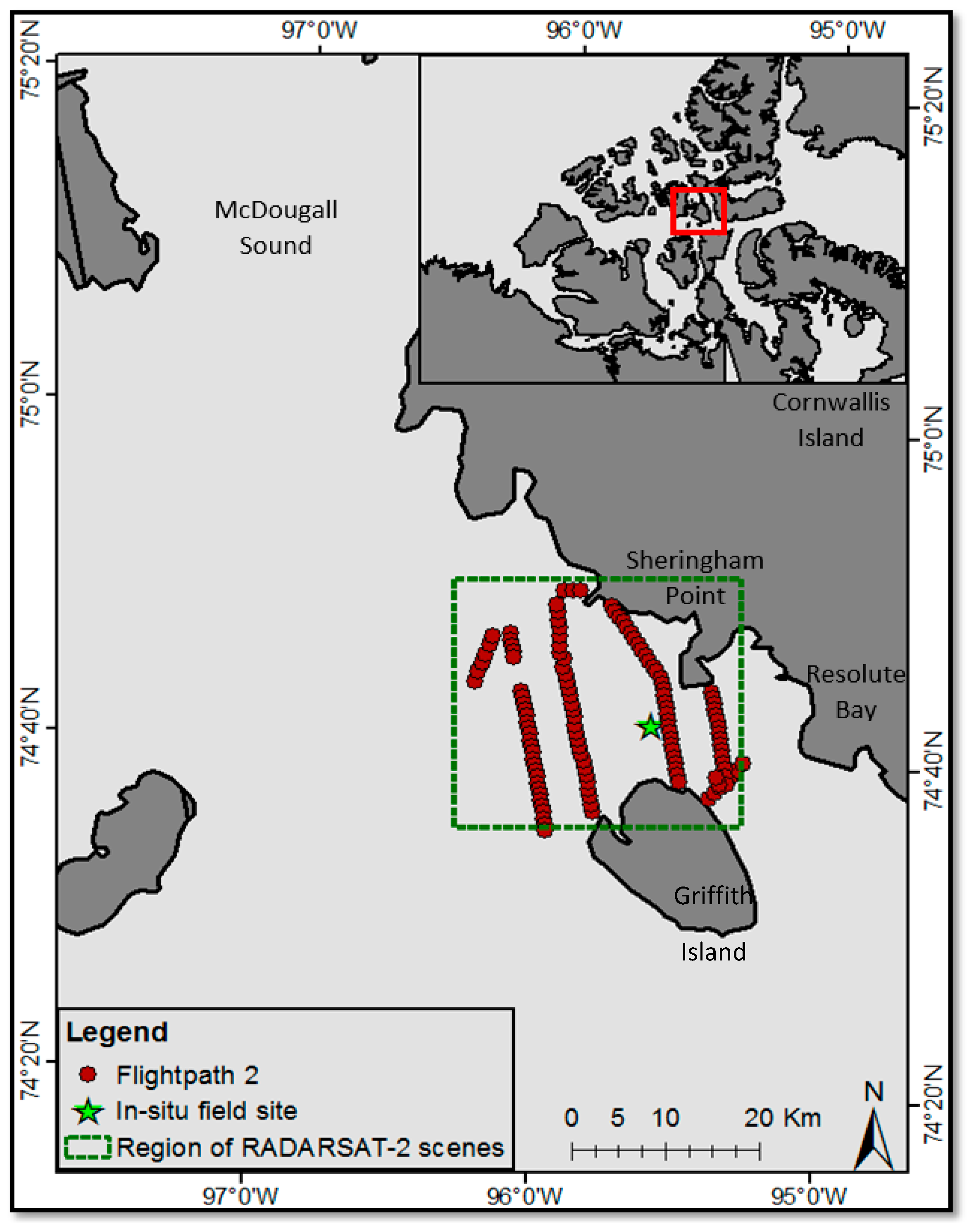
2.1. Study Area
2.2. Data
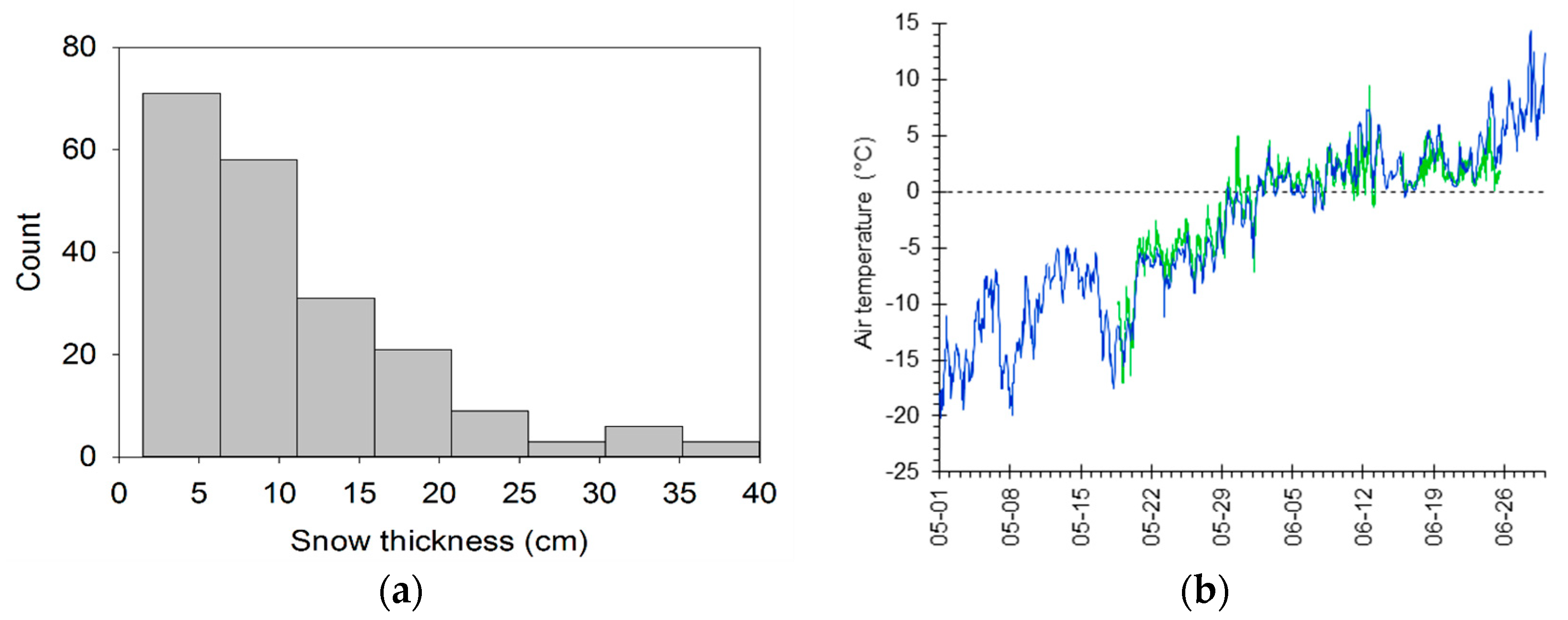
2.2.1. Aerial Surveys
2.2.2. RADARSAT-2 Data
2.3. Methods
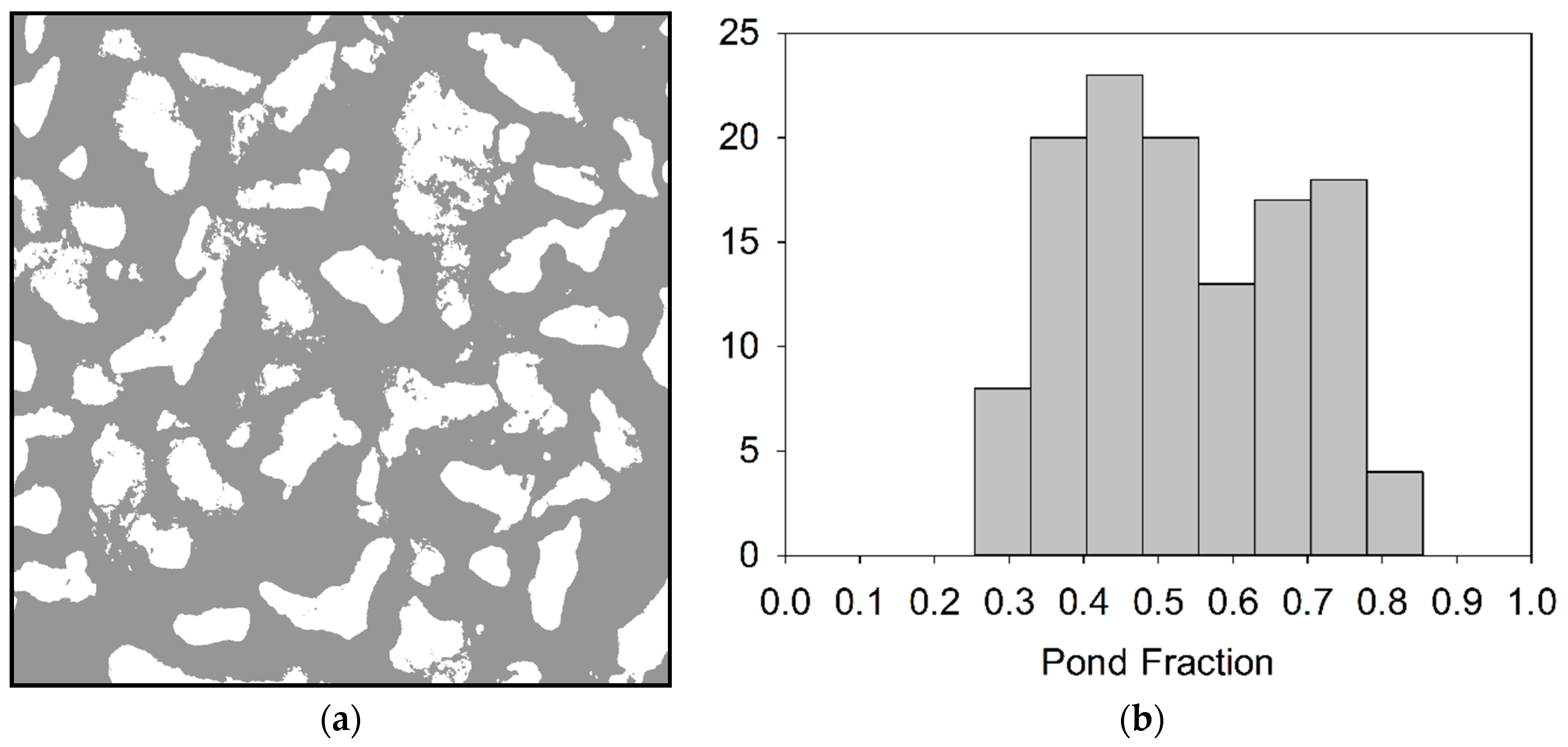
2.3.1. Estimation of Melt Pond Fraction from Aerial Photographs
2.3.2. RADARSAT-2 Data Processing
2.3.3. Image Sampling
2.3.4. Regression Model Development
2.3.5. Snow Thickness Images
3. Results and Discussion
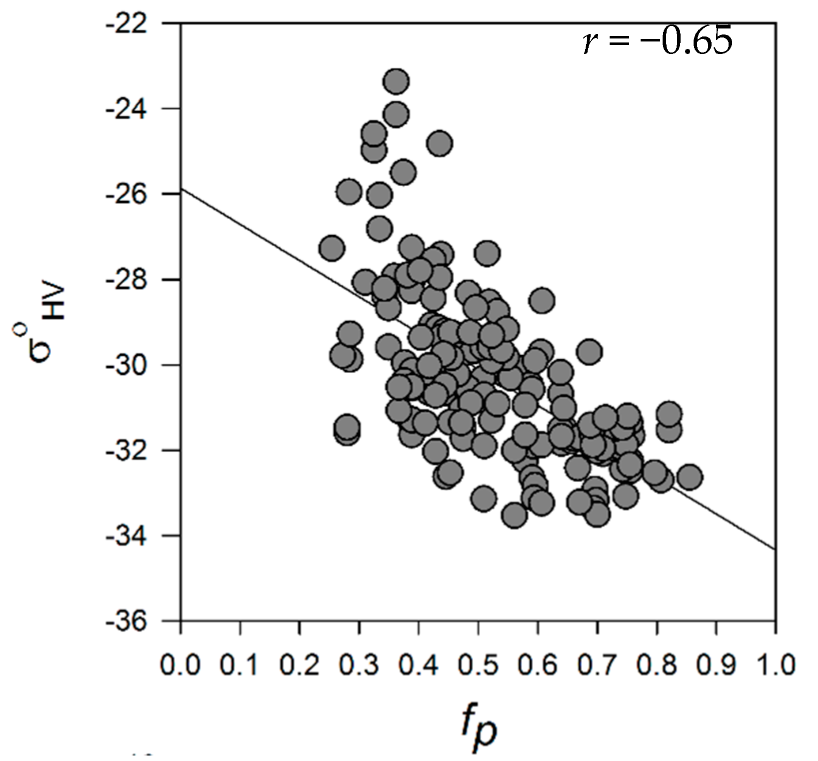
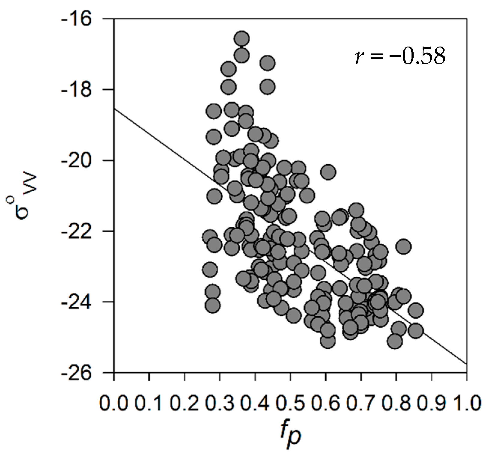
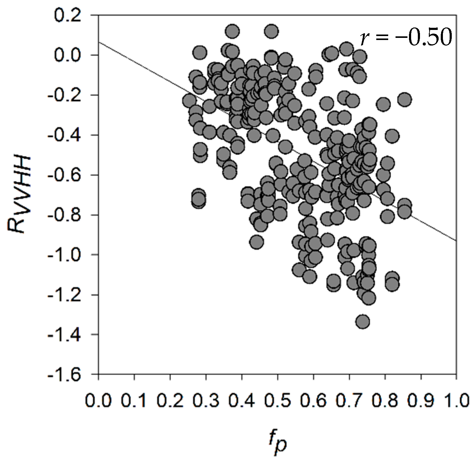
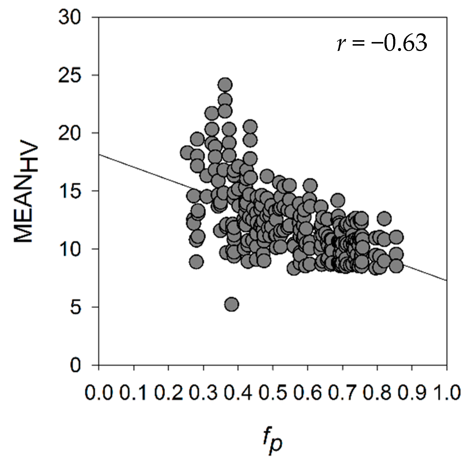
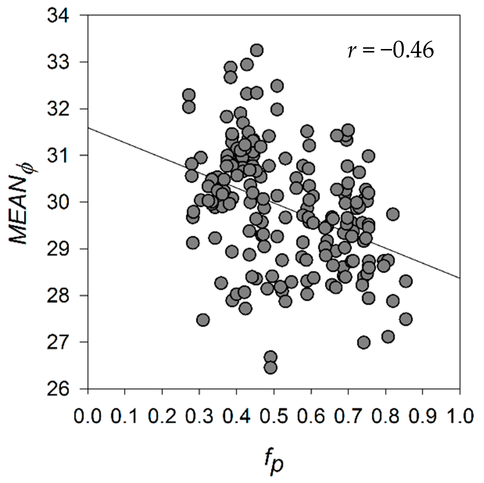
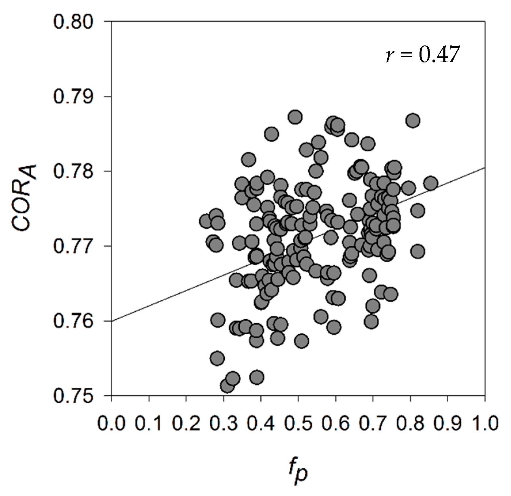
3.1. Relationship between Winter SAR Backscatter and Pond Fraction
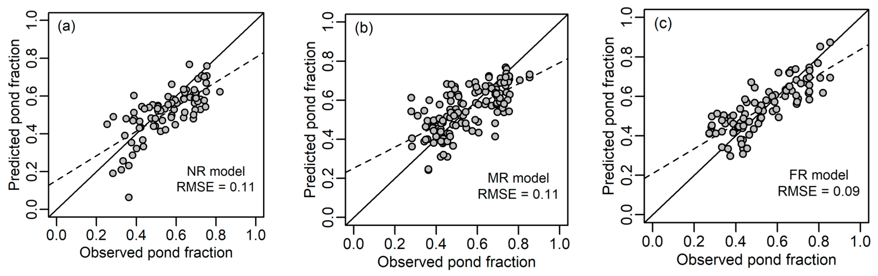
3.2. Prediction of Pond Fraction
3.3. Error Analysis
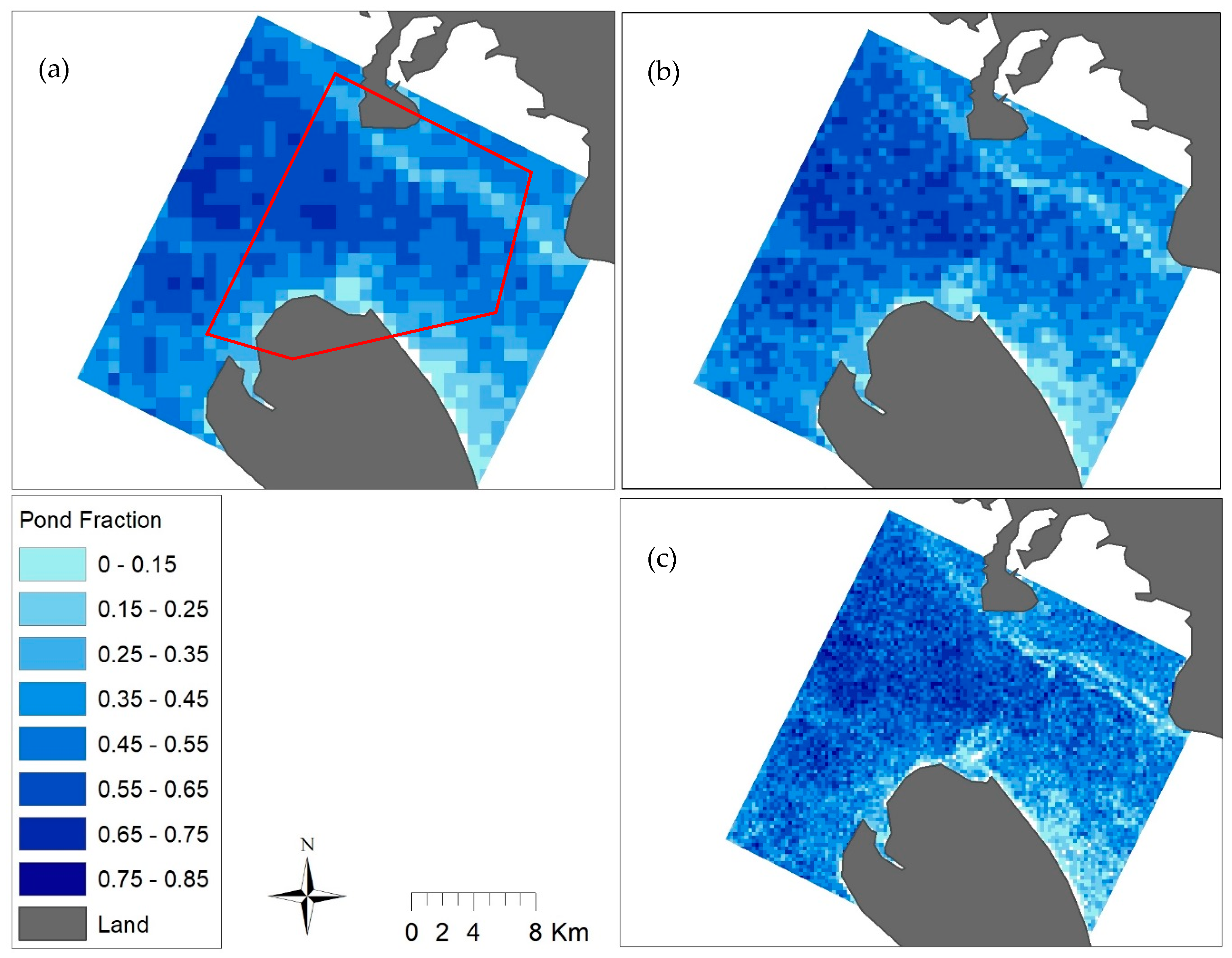
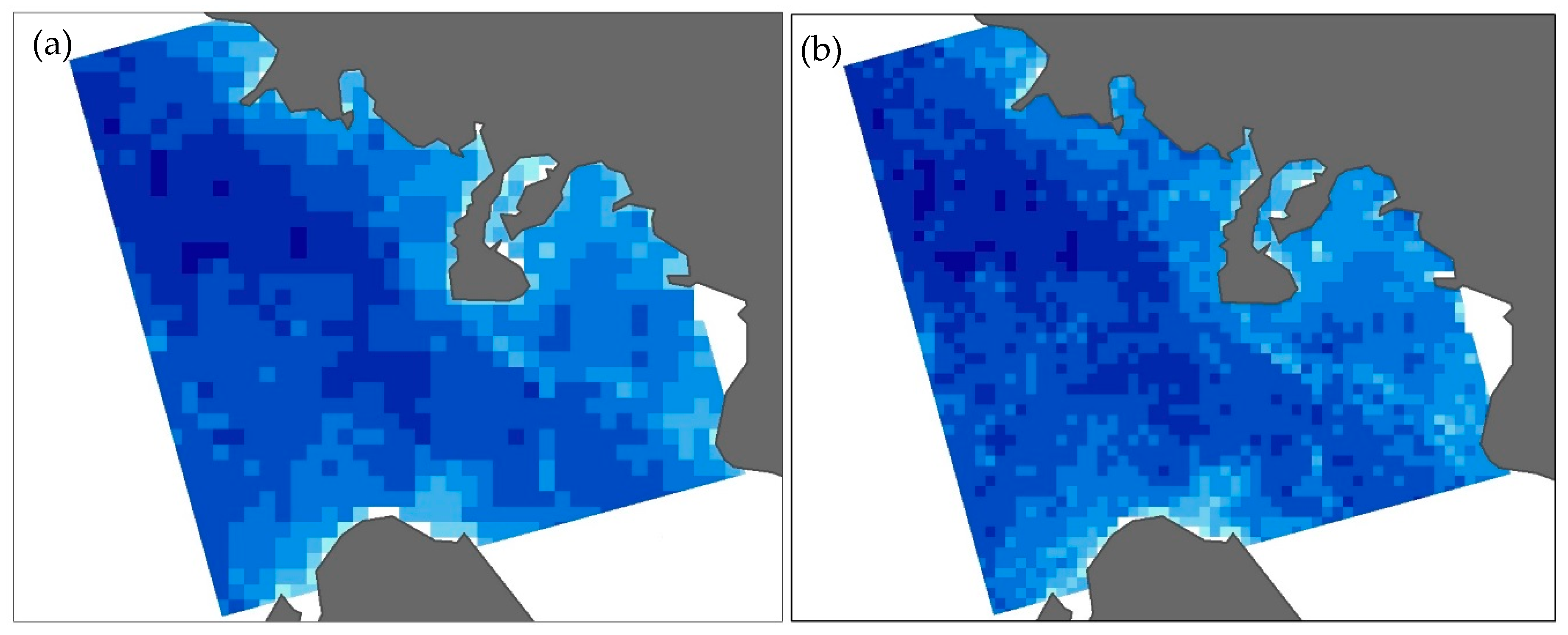
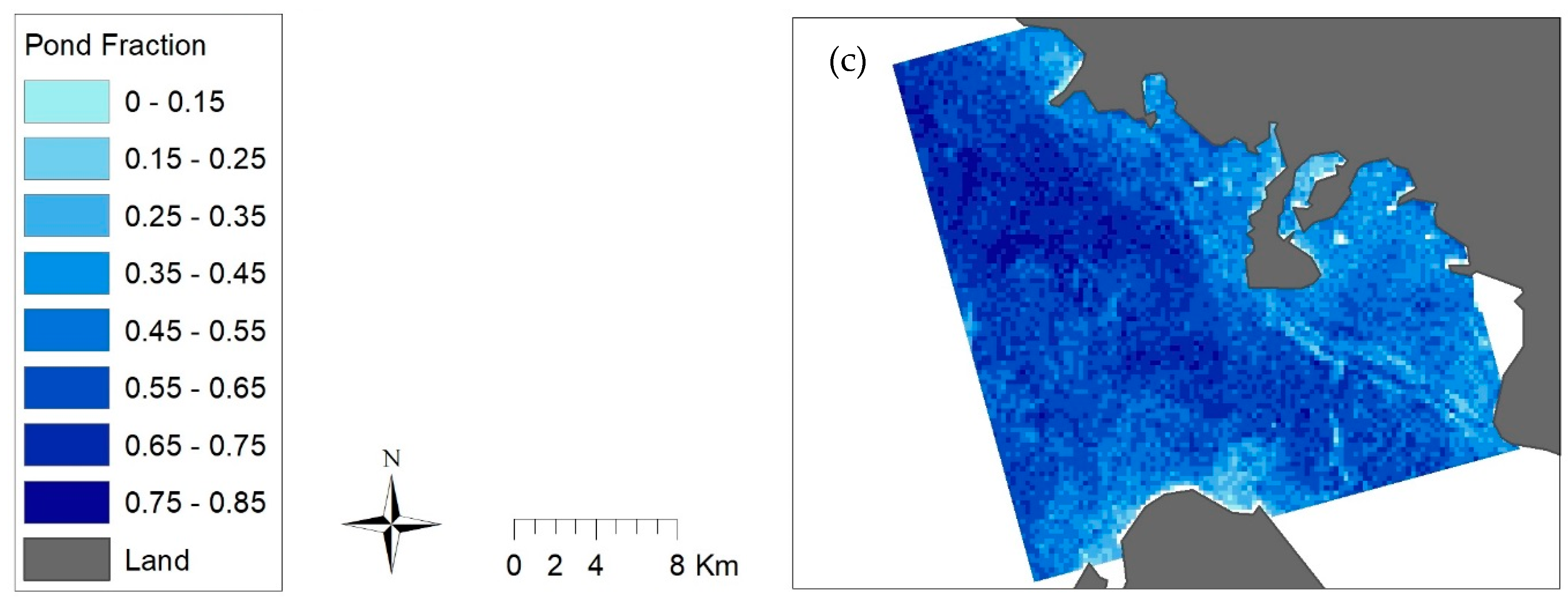
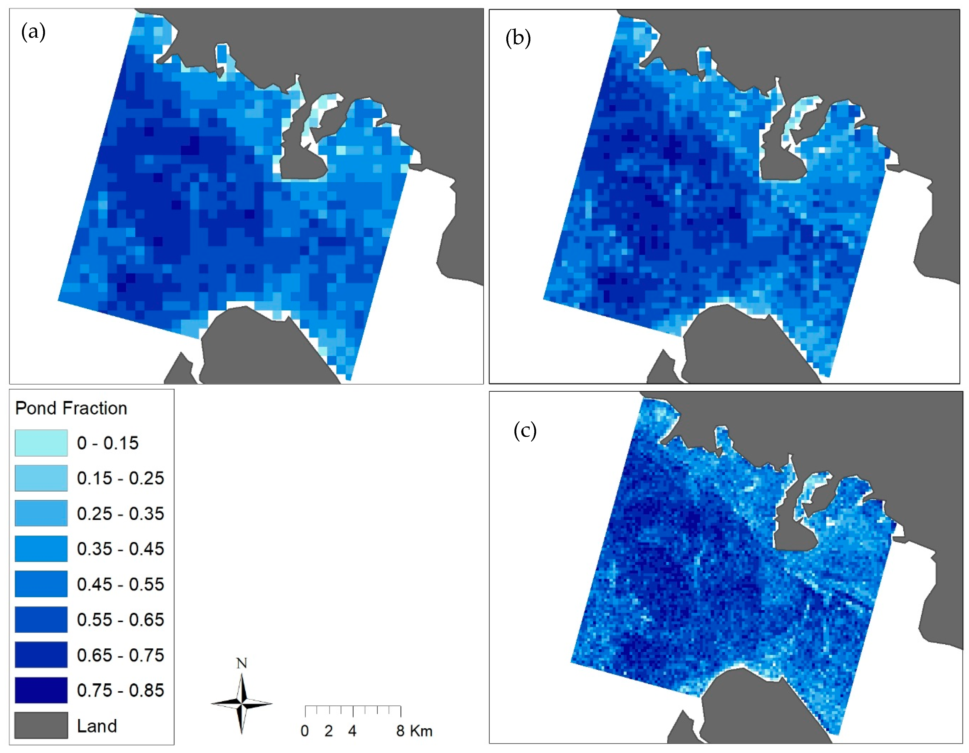
3.4. SAR Scene Pond Fraction Estimates
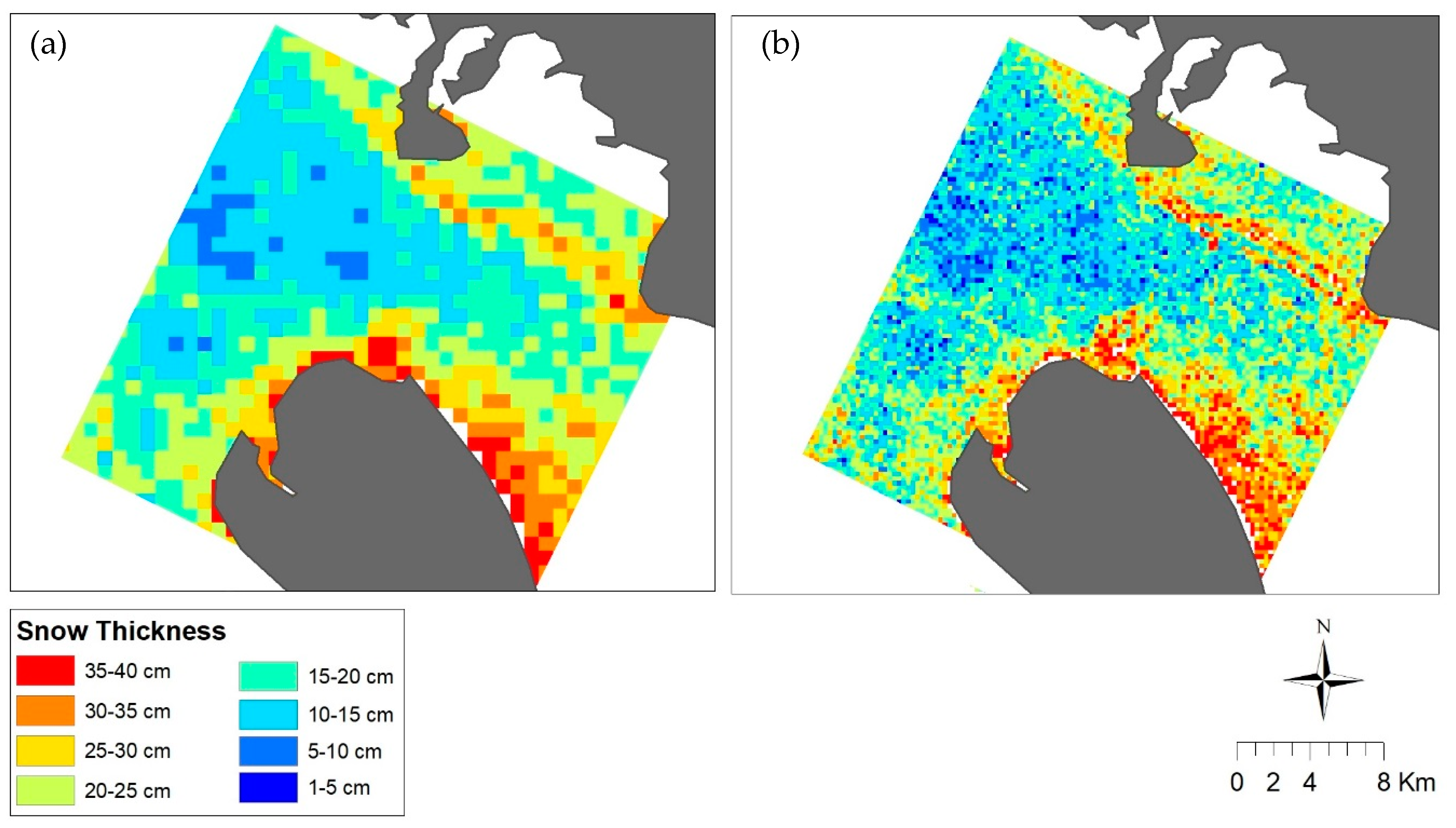
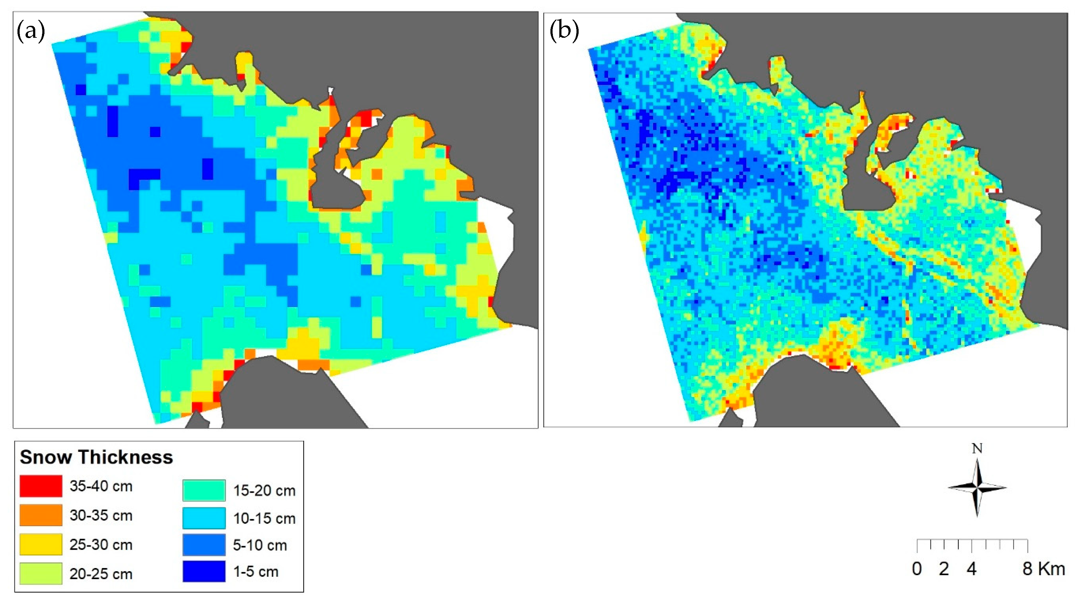
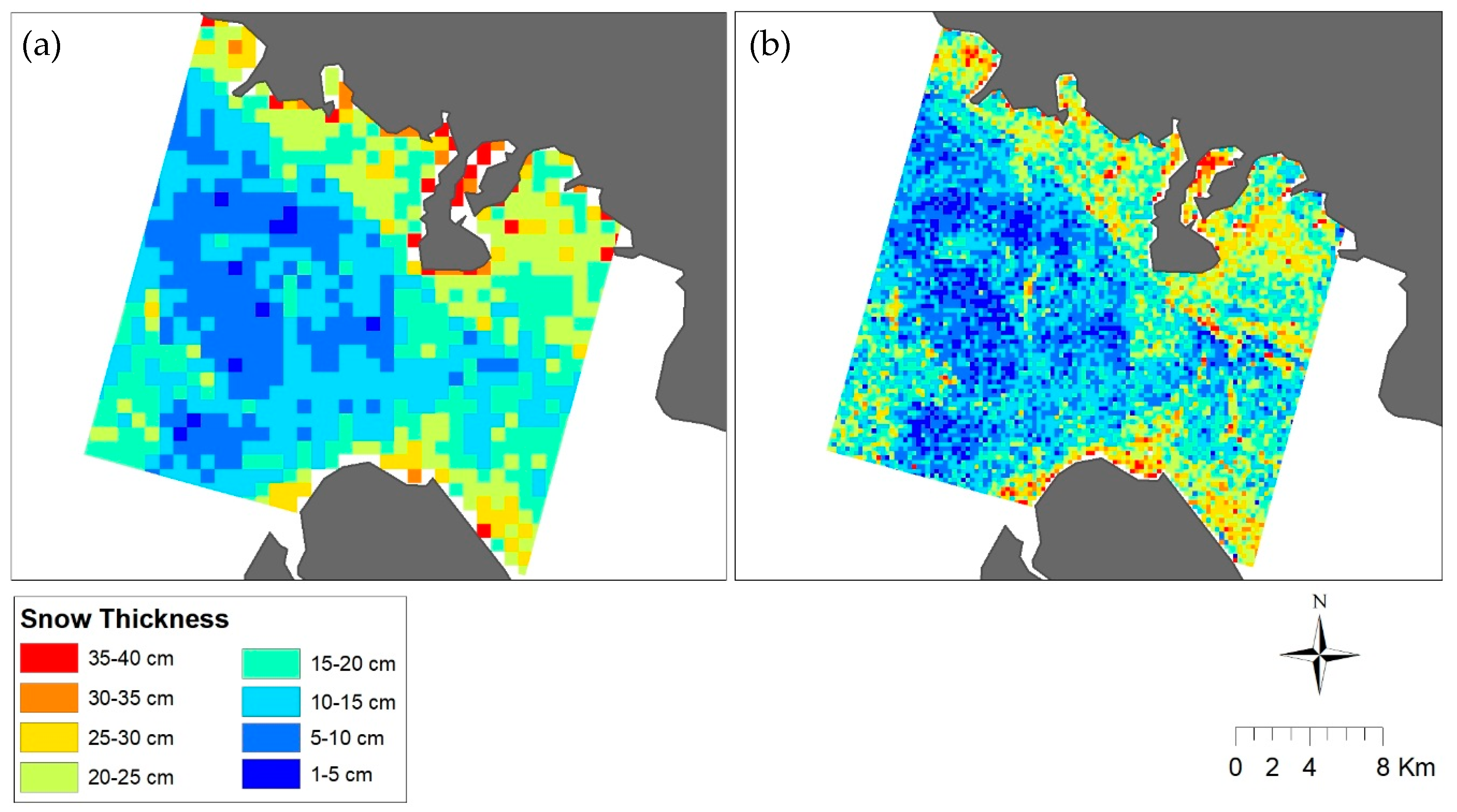
3.5. SAR-Based Estimation of Snow Thickness
4. Conclusions
Author Contributions
Funding
Acknowledgments
Conflicts of Interest
References
- Holt, B.; Digby, S.A. Processes and imagery of first-year fast sea ice during the melt season. J. Geophys. Res. Oceans 1985, 90, 5045–5062. [Google Scholar] [CrossRef]
- Barber, D.G.; Nghiem, S.V. The role of snow on the thermal dependence of microwave backscatter over sea ice. J. Geophys. Res. Oceans 1999, 104, 25789–25803. [Google Scholar]
- Yackel, J.J.; Barber, D.G.; Hanesiak, J.M. Melt ponds on sea ice in the Canadian Archipelago. I–Variability in morphological and radiative properties. J. Geophys. Res. 2000, 105, 22049–22060. [Google Scholar] [CrossRef]
- Scharien, R.K.; Yackel, J.J. Analysis of surface roughness and morphology of first-year sea ice melt ponds: Implications for microwave scattering. IEEE Trans. Geosci. Remote Sens. 2005, 43, 2927–2939. [Google Scholar] [CrossRef]
- Iacozza, J.; Barber, D.G. Ablation patterns of snow cover over smooth first-year sea ice in the Canadian Arctic. Hydrol. Process. 2001, 15, 3559–3569. [Google Scholar] [CrossRef]
- Eicken, H.; Krouse, H.R.; Kadko, D.; Perovich, D.K. Tracer studies of pathways and rates of meltwater transport through Arctic summer sea ice. J. Geophys. Res. Oceans 2002, 107. [Google Scholar] [CrossRef]
- Yackel, J.J.; Barber, D.G.; Papakyriakou, T.N.; Breneman, C. First-year Sea ice spring melt transitions in the Canadian Arctic Archipelago from time-series synthetic aperture radar data, 1992–2002. Hydrol. Process. 2007, 21, 253–265. [Google Scholar] [CrossRef]
- Polashenski, C.; Perovich, D.; Courville, Z. The mechanisms of sea ice melt pond formation and evolution. J. Geophys. Res. Oceans 2012, 117. [Google Scholar] [CrossRef]
- Iacozza, J.; Barber, D.G. An examination of snow redistribution over smooth land-fast sea ice. Hydrol. Process. 2010, 24, 850–865. [Google Scholar] [CrossRef]
- Iacozza, J.; Barber, D.G. An examination of the distribution of snow on sea-ice. Atmos. Ocean 1999, 37, 21–51. [Google Scholar]
- Webster, M.A.; Rigor, I.G.; Perovich, D.K.; Richter-Menge, J.A.; Polashenski, C.M.; Light, B. Seasonal evolution of melt ponds on Arctic sea ice. J. Geophys. Res. Oceans 2015, 120, 5968–5982. [Google Scholar] [CrossRef]
- Landy, J.; Ehn, J.; Shields, M.; Barber, D. Surface and melt pond evolution on landfast first-year sea ice in the Canadian Arctic Archipelago. J. Geophys. Res. Oceans 2014, 119, 3054–3075. [Google Scholar] [CrossRef]
- Markus, T.; Cavalieri, D.J.; Tschudi, M.A.; Ivanoff, A. Comparison of aerial video and Landsat 7 data over ponded sea ice. Remote Sens. Environ. 2003, 86, 458–469. [Google Scholar] [CrossRef]
- Tschudi, M.A.; Maslanik, J.A.; Perovich, D.K. Derivation of melt pond coverage on Arctic sea ice using MODIS observations. Remote Sens. Environ. 2008, 112, 2605–2614. [Google Scholar] [CrossRef]
- Rösel, A.; Kaleschke, L.; Birnbaum, G. Melt ponds on Arctic sea ice determined from MODIS satellite data using an artificial neural network. Cryosphere 2012, 6, 431–446. [Google Scholar] [CrossRef]
- Zege, E.; Malinka, A.; Katsev, I.; Prikhach, A.; Heygster, G.; Istomina, L.; Schwarz, P. Algorithm to retrieve the melt pond fraction and the spectral albedo of Arctic summer ice from satellite optical data. Remote Sens. Environ. 2015, 163, 153–164. [Google Scholar] [CrossRef]
- Istomina, L.; Heygster, G.; Huntemann, M.; Schwarz, P.; Birnbaum, G.; Scharien, R.; Polashenski, C.; Perovich, D.; Zege, E.; Malinka, A.; et al. Melt pond fraction and spectral sea ice albedo retrieval from MERIS data-Part 1: Validation against in situ, aerial, and ship cruise data. Cryosphere 2015, 9, 1551–1566. [Google Scholar] [CrossRef]
- Istomina, L.; Heygster, G.; Huntemann, M.; Marks, H.; Melsheimer, C.; Zege, E.; Malinka, A.; Prikhach, A.; Katsev, I. Melt pond fraction and spectral sea ice albedo retrieval from MERIS data–Part 2: Case studies and trends of sea ice albedo and melt ponds in the Arctic for years 2002–2011. Cryosphere 2015, 9, 1567–1578. [Google Scholar] [CrossRef]
- Tanaka, Y.; Tateyama, K.; Kameda, T.; Hutchings, J.K. Estimation of melt pond fraction over high-concentration Arctic sea ice using AMSR-E passive microwave data. J. Geophys. Res. Oceans 2016, 121, 7056–7072. [Google Scholar] [CrossRef]
- Barber, D.G.; Yackel, J. The physical, radiative and microwave scattering characteristics of melt ponds on Arctic landfast sea ice. Int. J. Remote Sens. 1999, 20, 2069–2090. [Google Scholar] [CrossRef]
- Mäkynen, M.; Kern, S.; Rösel, A.; Pedersen, L.T. On the estimation of melt pond fraction on the Arctic Sea ice with ENVISAT WSM images. IEEE Trans. Geosci. Remote Sens. 2014, 52, 7366–7379. [Google Scholar] [CrossRef]
- Scharien, R.K.; Landy, J.; Barber, D.G. First-year sea ice melt pond fraction estimation from dual-polarisation C-band SAR—Part 1: In situ observations. Cryosphere 2014, 8, 2147–2162. [Google Scholar] [CrossRef]
- Fors, A.S.; Divine, D.V.; Doulgeris, A.P.; Renner, A.H.; Gerland, S. Signature of Arctic first-year ice melt pond fraction in X-band SAR imagery. Cryosphere 2017, 11, 755–771. [Google Scholar] [CrossRef]
- Scharien, R.K.; Segal, R.; Nasonova, S.; Nandan, V.; Howell, S.E.; Haas, C. Winter Sentinel-1 backscatter as a predictor of spring Arctic sea ice melt pond fraction. Geophys. Res. Lett. 2017, 44. [Google Scholar] [CrossRef]
- Scharien, R.; Segal, R.; Yackel, J.; Howell, S.; Nasonova, S. Linking winter and spring thermodynamic sea-ice states at critical scales using an object-based image analysis of Sentinel-1. Ann. Glaciol. 2017, 59, 1–15. [Google Scholar] [CrossRef]
- Derksen, C.; Piwowar, J.; LeDrew, E. Sea-ice melt-pond fraction as determined from low level aerial photographs. Arct. Alp. Res. 1997, 29, 345–351. [Google Scholar] [CrossRef]
- Tschudi, M.A.; Curry, J.A.; Maslanik, J.A. Determination of areal surface-feature coverage in the Beaufort Sea using aircraft video data. Ann. Glaciol. 1997, 25, 434–438. [Google Scholar] [CrossRef]
- Barber, D.G.; Papakyriakou, T.N.; LeDrew, E.F. On the relationship between energy fluxes, dielectric properties, and microwave scattering over snow covered first-year sea ice during the spring transition period. J. Geophys. Res. Oceans 1994, 99, 22401–22411. [Google Scholar] [CrossRef]
- Barber, D.G.; Reddan, S.P.; LeDrew, E.F. Statistical characterization of the geophysical and electrical properties of snow on landfast first-year sea ice. J. Geophys. Res. Oceans 1995, 100, 2673–2686. [Google Scholar] [CrossRef]
- Sturm, M.; Holmgren, J.; Perovich, D.K. Winter snow cover on the sea ice of the Arctic Ocean at the Surface Heat Budget of the Arctic Ocean (SHEBA): Temporal evolution and spatial variability. J. Geophys. Res. Oceans 2002, 107. [Google Scholar] [CrossRef]
- Bredow, J.W.; Gogineni, S. Comparison of measurements and theory for backscatter from bare and snow-covered saline ice. IEEE Trans. Geosci. Remote Sens. 1990, 28, 456–463. [Google Scholar] [CrossRef]
- Lytle, V.I.; Jezek, K.C.; Hosseinmostafa, A.R.; Gogineni, S.P. Laboratory backscatter measurements over urea ice with a snow cover at Ku band. IEEE Trans. Geosci. Remote Sens. 1993, 31, 1009–1016. [Google Scholar] [CrossRef]
- Markus, T.; Cavalieri, D.J. Snow depth distribution over sea ice in the Southern Ocean from satellite passive microwave data. In Antarctic Sea Ice: Physical Processes, Interactions and Variability; Wiley Online Library: Hoboken, NJ, USA, 1998; Volume 74, pp. 19–39. [Google Scholar]
- Cavalieri, D.J.; Markus, T.; Ivanoff, A.; Miller, J.A.; Brucker, L.; Sturm, M.; Maslanik, J.A.; Heinrichs, J.F.; Gasiewski, A.J.; Leuschen, C.; et al. A comparison of snow depth on sea ice retrievals using airborne altimeters and an AMSR-E simulator. IEEE Trans. Geosci. Remote Sens. 2012, 50, 3027–3040. [Google Scholar] [CrossRef]
- Maass, N.; Kaleschke, L.; Tian-Kunze, X.; Drusch, M. Snow thickness retrieval over thick Arctic sea ice using SMOS satellite data. Cryosphere 2013, 7, 1971–1989. [Google Scholar] [CrossRef]
- Kurtz, N.T.; Farrell, S.L.; Studinger, M.; Galin, N.; Harbeck, J.P.; Lindsay, R.; Onana, V.D.; Panzer, B.; Sonntag, J.G. Sea ice thickness, freeboard, and snow depth products from Operation IceBridge airborne data. Cryosphere 2013, 7, 1035–1056. [Google Scholar] [CrossRef]
- Kwok, R.; Kurtz, N.T.; Brucker, L.; Ivanoff, A.; Newman, T.; Farrell, S.L.; King, J.; Howell, S.; Webster, M.A.; Paden, J.; et al. Intercomparison of snow depth retrievals over Arctic sea ice from radar data acquired by Operation IceBridge. Cryosphere 2017, 11. [Google Scholar] [CrossRef]
- Barber, D.G.; Fung, A.K.; Grenfell, T.C.; Nghiem, S.V.; Onstott, R.G.; Lytle, V.I.; Perovich, D.K.; Gow, A.J. The role of snow on microwave emission and scattering over first-year sea ice. IEEE Trans. Geosci. Remote Sens. 1998, 36, 1750–1763. [Google Scholar] [CrossRef]
- Gill, J.P.; Yackel, J.J.; Geldsetzer, T.; Fuller, M.C. Sensitivity of C-band synthetic aperture radar polarimetric parameters to snow thickness over land fast smooth first-year sea ice. Remote Sens. Environ. 2015, 166, 34–49. [Google Scholar] [CrossRef]
- Zheng, J.; Geldsetzer, T.; Yackel, J. Snow thickness estimation on first-year sea ice using microwave and optical remote sensing with melt modelling. Remote Sens. Environ. 2017, 199, 321–332. [Google Scholar] [CrossRef]
- Kim, Y.S.; Onstott, R.; Moore, R. Effect of a snow cover on microwave backscatter from sea ice. IEEE J. Ocean. Eng. 1984, 9, 383–388. [Google Scholar]
- Tjuatja, S.; Fung, A.K.; Bredow, J. A scattering model for snow-covered sea ice. IEEE Trans. Geosci. Remote Sens. 1992, 30, 804–810. [Google Scholar] [CrossRef]
- Dierking, W.; Pettersson, M.I.; Askne, J. Multifrequency scatterometer measurements of Baltic Sea ice during EMAC-95. Int. J. Remote Sens. 1999, 20, 349–372. [Google Scholar] [CrossRef]
- Wakabayashi, H.; Matsuoka, T.; Nakamura, K.; Nishio, F. Polarimetric characteristics of sea ice in the Sea of Okhotsk observed by airborne L-band SAR. IEEE Trans. Geosci. Remote Sens. 2004, 42, 2412–2425. [Google Scholar] [CrossRef]
- Scheuchl, B.; Cumming, I.; Hajnsek, I. Classification of fully polarimetric single-and dual-frequency SAR data of sea ice using the Wishart statistics. Can. J. Remote Sens. 2005, 31, 61–72. [Google Scholar] [CrossRef]
- Gill, J.P.; Yackel, J.J. Evaluation of C-band SAR polarimetric parameters for discrimination of first-year sea ice types. Can. J. Remote Sens. 2012, 38, 306–323. [Google Scholar] [CrossRef]
- Gill, J.P.; Yackel, J.J.; Geldsetzer, T. Analysis of consistency in first-year sea ice classification potential of C-band SAR polarimetric parameters. Can. J. Remote Sens. 2013, 39, 101–117. [Google Scholar] [CrossRef]
- Holmes, Q.A.; Nuesch, D.R.; Shuchman, R.A. Textural analysis and real-time classification of sea-ice types using digital SAR data. IEEE Trans. Geosci. Remote Sens. 1984, 22, 113–120. [Google Scholar] [CrossRef]
- Shokr, M.E. Evaluation of second-order texture parameters for sea ice classification from radar images. J. Geophys. Res. Oceans 1991, 96, 10625–10640. [Google Scholar] [CrossRef]
- Clausi, D.A. An analysis of co-occurrence texture statistics as a function of grey level quantization. Can. J. Remote Sens. 2002, 28, 45–62. [Google Scholar] [CrossRef]
- Liu, H.; Guo, H.; Zhang, L. SVM-based sea ice classification using textural features and concentration from RADARSAT-2 Dual-Pol ScanSAR data. IEEE J. Sel. Top. Appl. Earth Obs. Remote Sens. 2015, 8, 1601–1613. [Google Scholar] [CrossRef]
- Haralick, R.M.; Shanmugam, K. Textural features for image classification. IEEE Syst. Man Cybern. Mag. 1973, 6, 610–621. [Google Scholar] [CrossRef]
- Barber, D.; LeDrew, E. SAR sea ice discrimination using texture statistics—A multivariate approach. Photogramm. Eng. Remote Sens. 1991, 57, 385–395. [Google Scholar]
- Soh, L.K.; Tsatsoulis, C. Texture analysis of SAR sea ice imagery using gray level co-occurrence matrices. IEEE Trans. Geosci. Remote Sens. 1999, 37, 780–795. [Google Scholar] [CrossRef]
- Lee, J.S.; Wen, J.H.; Ainsworth, T.L.; Chen, K.S.; Chen, A.J. Improved sigma filter for speckle filtering of SAR imagery. IEEE Trans. Geosci. Remote Sens. 2009, 47, 202–213. [Google Scholar]
- Oliver, C.; Quegan, S. Understanding Synthetic Aperture Radar Images; SciTech Publishing: Stevenage, UK, 2004. [Google Scholar]
- Drinkwater, M.R.; Kwok, R.; Rignot, E.; Israelsson, H.; Onstott, R.G.; Winebrenner, D.P. Potential applications of polarimetry to the classification of sea ice. In Microwave Remote Sensing of Sea Ice; Carsey, F.D., Ed.; American Geophysical Union: Washington, DC, USA, 1992; pp. 419–428. [Google Scholar]
- Cloude, S.R.; Pottier, E. An entropy based classification scheme for land applications of polarimetric SAR. IEEE Trans. Geosci. Remote Sens. 1997, 35, 68–78. [Google Scholar] [CrossRef]
- Baraldi, A.; Parmiggiani, F. An investigation of the textural characteristics associated with gray level cooccurrence matrix statistical parameters. IEEE Trans. Geosci. Remote Sens. 1995, 33, 293–304. [Google Scholar] [CrossRef]
- Hirose, T.K.; McNutt, L.; Paterson, J.S. A Study of Textoral and Tonal Information for Classifying Sea Ice from SAR Imagery. In 12th Canadian Symposium on Remote Sensing Geoscience and Remote Sensing Symposium, Proceedings of International Geoscience and Remote Sensing Symposium IGARSS 1989, Vancouver, BC, Canada, 10–14 July 1989; IEEE: New York, NY, USA, 1989; pp. 747–750. [Google Scholar]
- Newsam, S.D.; Kamath, C. Retrieval Using Texture Features in High Resolution Multi-Spectral Satellite Imagery (No. UCRL-CONF-201981); Lawrence Livermore National Laboratory (LLNL): Livermore, CA, USA, 2004.
- Gong, P.; Marceau, D.J.; Howarth, P.J. A comparison of spatial feature extraction algorithms for land-use classification with SPOT HRV data. Remote Sens. Environ. 1992, 40, 137–151. [Google Scholar] [CrossRef]
- Cossu, R. Segmentation by means of textural analysis. Pixel 1988, 1, 21–24. [Google Scholar]
- Liew, S.C.; Lim, H.; Kwoh, L.K.; Tay, G.K. Texture analysis of SAR images. In 1995 International Geoscience and Remote Sensing Symposium, IGARSS ’95. Quantitative Remote Sensing for Science and Applications, Proceedings of International Geoscience and Remote Sensing Symposium IGARSS 1995, Firenze, Italy, 10–14 July 1995; IEEE: New York, NY, USA, 1995; pp. 1412–1414. [Google Scholar]
- Hall-Beyer, M. GLCM Texture: A Tutorial, Version 2.10. 2007. Available online: https://www.ucalgary.ca/mhallbey/tutorial-glcm-texture (accessed on 20 January 2018).
- Breiman, L. Random Forests. Mach. Learn. 2001, 45, 5–32. [Google Scholar] [CrossRef]
- Millard, K.; Richardson, M. On the importance of training data sample selection in random forest image classification: A case study in peatland ecosystem mapping. Remote Sens. 2015, 7, 8489–8515. [Google Scholar] [CrossRef]
- Torres, R.; Buck, C.; Guijarro, J.; Suchail, J.L.; Schönenberg, A. The envisat ASAR instrument verification and characterisation. In Proceedings of the SAR workshop: CEOS Committee on Earth Observation Satellites, Toulouse, France, 26–29 October 1999; pp. 303–310. [Google Scholar]
- Torres, R.; Snoeij, P.; Geudtner, D.; Bibby, D.; Davidson, M.; Attema, E.; Traver, I.N. GMES Sentinel-1 mission. Remote Sens. Environ. 2012, 120, 9–24. [Google Scholar] [CrossRef]
- Nandan, V.; Scharien, R.; Geldsetzer, T.; Mahmud, M.; Yackel, J.J.; Islam, T.; Duguay, C. Geophysical and atmospheric controls on Ku-, X-and C-band backscatter evolution from a saline snow cover on first-year sea ice from late-winter to pre-early melt. Remote Sens. Environ. 2017, 198, 425–441. [Google Scholar] [CrossRef]
- Scheuchl, B.; Flett, D.; Caves, R.; Cumming, I. Potential of RADARSAT-2 data for operational sea ice monitoring. Can. J. Remote Sens. 2004, 30, 448–461. [Google Scholar] [CrossRef]
- Onstott, R.G. SAR and scatterometer signatures of sea ice. In Microwave Remote Sensing of Sea Ice; Carsey, F.D., Ed.; American Geophysical Union: Washington, DC, USA, 1992; pp. 73–104. [Google Scholar]
- Fung, A.K.; Eom, H.J. Application of a combined rough surface and volume scattering theory to sea ice and snow backscatter. IEEE Trans. Geosci. Remote Sens. 1982, 4, 528–536. [Google Scholar] [CrossRef]
- Lewis, A.J.; Henderson, F.M.; Holcomb, D.W. Radar fundamentals: the geoscience perspective. In Principles & Applications of Imaging Radar. Manual of Remote Sensing, 3rd ed.; Wiley: Hoboken, NJ, USA, 1998; Volume 3, pp. 131–180. [Google Scholar]
- Nandan, V.; Geldsetzer, T.; Yackel, J.; Mahmud, M.; Scharien, R.; Howell, S.; King, J.; Ricker, R.; Else, B. Effect of Snow Salinity on CryoSat-2 Arctic First- Year Sea Ice Freeboard Measurements. Geophys. Res. Lett. 2017, 44. [Google Scholar] [CrossRef]
- Sturm, M.; Liston, G.E.; Benson, C.S.; Holmgren, J. Characteristics and growth of a snowdrift in Arctic Alaska, USA. Arct. Antarct. Alp. Res. 2001, 33, 319–329. [Google Scholar] [CrossRef]
- Dierking, W.; Dall, J. Sea-ice deformation state from synthetic aperture radar imagery—Part I: Comparison of C-and L-band and different polarization. IEEE Trans. Geosci. Remote Sens. 2007, 45, 3610–3622. [Google Scholar] [CrossRef]


| SAR Scene | Acquisition Date (yyyy-mm-dd) | Incidence Angle (Range) | Number of Aerial Photographs |
|---|---|---|---|
| FQ4 | 2012-05-10 | 23.1° (NR) | 78 |
| FQ8 | 2012-05-24 | 27.8° (NR) | 97 |
| FQ13 | 2012-05-21 | 33.2° (MR) | 97 |
| FQ15 | 2012-05-21 | 35.2° (MR) | 87 |
| FQ18 | 2012-05-18 | 38.1° (MR) | 102 |
| FQ22 | 2012-05-17 | 41.7° (FR) | 87 |
| FQ23 | 2012-05-15 | 42.6° (FR) | 102 |
| Nomenclature | Notation | Reference |
|---|---|---|
| Co-polarized power (horizontal) (in dB) | (linear) | [57] |
| Co-polarized power (vertical) (in dB) | (linear) | |
| Cross-polarized power (in dB) | (linear) | |
| Co-polarized ratio (in dB) | (linear) | |
| Co-polarized phase difference | (polarimetric) | |
| Co-polarized correlation co-efficient | (polarimetric) | |
| Entropy | (polarimetric) | [58] |
| Anisotropy | (polarimetric) | |
| Alpha angle | (polarimetric) |
| Terminology | Theoretical Description | References |
|---|---|---|
| Entropy (ENT) | Detects the randomness of grey level distribution. Entropy will be higher for nearly random or noisy images. | [59] |
| Angular second moment (ASM) | Detects disorder in texture. High energy values represent the constant of periodic form of gray level distribution | [53,60] |
| Contrast (CON) | The difference between the highest and the lowest values of a connecting set of pixels. Contrast is greater for images that have rapidly fluctuating intensities. | [61] |
| GLCM variance (VAR) | The degree of heterogeneity. Variance increases when the gray level values differ from their mean. | [62] |
| Correlation (COR) | Measures linear-dependencies of gray tone in the image. | [63] |
| Homogeneity (HOM) | Gives maximum value when all elements in the image are same. | [49] |
| Dissimilarity (DIS) | Assists to distinguish most surface features. | [64] |
| GLCM Mean (MEAN) | Measures the mean of Grey level co-occurrences values. Generally least correlated with other texture parameters. | [65] |
| NR Parameters | r | MR Parameters | r | FR Parameters | r |
|---|---|---|---|---|---|
| −0.652 | −0.627 | −0.584 | |||
| −0.540 | −0.579 | −0.550 | |||
| −0.532 | −0.552 | −0.540 | |||
| 0.473 | 0.500 | −0.501 | |||
| −0.336 | −0.497 | −0.464 | |||
| −0.323 | −0.427 | 0.440 | |||
| 0.304 | −0.361 | 0.382 | |||
| −0.285 | −0.351 | 0.364 | |||
| −0.271 | −0.344 | −0.312 | |||
| −0.253 | −0.299 | −0.293 | |||
| −0.224 | −0.285 | −0.211 | |||
| −0.196 | −0.259 | −0.156 | |||
| −0.177 | −0.242 | −0.116 | |||
| 0.164 | −0.241 | −0.105 | |||
| −0.135 | −0.229 | −0.072 | |||
| 0.080 | −0.206 | 0.066 | |||
| 0.065 | −0.180 | −0.058 | |||
| −0.164 | −0.052 | ||||
| 0.154 | −0.04 | ||||
| 0.152 | |||||
| 0.113 | |||||
| −0.105 | |||||
| 0.073 | |||||
| −0.050 | |||||
| 0.042 |
| NR | IncMSE | MR | IncMSE | FR | IncMSE |
|---|---|---|---|---|---|
| 0.0116 | 0.0058 | 0.0046 | |||
| 0.0036 | 0.0038 | 0.0039 | |||
| 0.0015 | 0.0036 | 0.0035 | |||
| 0.0010 | 0.0029 | 0.0021 | |||
| 0.0010 | 0.0021 | 0.0018 | |||
| 0.0009 | 0.0021 | 0.0017 | |||
| 0.0009 | 0.0017 | 0.0008 | |||
| 0.0005 | 0.0013 | 0.0007 | |||
| 0.0004 | 0.0012 | 0.0006 | |||
| 0.0004 | 0.0008 | 0.0003 | |||
| 0.0004 | 0.0007 | 0.0002 | |||
| 0.0003 | 0.0006 | 0.0002 | |||
| 0.0002 | 0.0005 | 0.0002 |
© 2018 by the authors. Licensee MDPI, Basel, Switzerland. This article is an open access article distributed under the terms and conditions of the Creative Commons Attribution (CC BY) license (http://creativecommons.org/licenses/by/4.0/).
Share and Cite
Ramjan, S.; Geldsetzer, T.; Scharien, R.; Yackel, J. Predicting Melt Pond Fraction on Landfast Snow Covered First Year Sea Ice from Winter C-Band SAR Backscatter Utilizing Linear, Polarimetric and Texture Parameters. Remote Sens. 2018, 10, 1603. https://doi.org/10.3390/rs10101603
Ramjan S, Geldsetzer T, Scharien R, Yackel J. Predicting Melt Pond Fraction on Landfast Snow Covered First Year Sea Ice from Winter C-Band SAR Backscatter Utilizing Linear, Polarimetric and Texture Parameters. Remote Sensing. 2018; 10(10):1603. https://doi.org/10.3390/rs10101603
Chicago/Turabian StyleRamjan, Saroat, Torsten Geldsetzer, Randall Scharien, and John Yackel. 2018. "Predicting Melt Pond Fraction on Landfast Snow Covered First Year Sea Ice from Winter C-Band SAR Backscatter Utilizing Linear, Polarimetric and Texture Parameters" Remote Sensing 10, no. 10: 1603. https://doi.org/10.3390/rs10101603
APA StyleRamjan, S., Geldsetzer, T., Scharien, R., & Yackel, J. (2018). Predicting Melt Pond Fraction on Landfast Snow Covered First Year Sea Ice from Winter C-Band SAR Backscatter Utilizing Linear, Polarimetric and Texture Parameters. Remote Sensing, 10(10), 1603. https://doi.org/10.3390/rs10101603