Attention-Mechanism-Containing Neural Networks for High-Resolution Remote Sensing Image Classification

Abstract

A deep neural network is suitable for remote sensing image pixel-wise classification because it effectively extracts features from the raw data. However, remote sensing images with higher spatial resolution exhibit smaller inter-class differences and greater intra-class differences; thus, feature extraction becomes more difficult. The attention mechanism, as a method that simulates the manner in which humans comprehend and perceive images, is useful for the quick and accurate acquisition of key features. In this study, we propose a novel neural network that incorporates two kinds of attention mechanisms in its mask and trunk branches; i.e., control gate (soft) and feedback attention mechanisms, respectively, based on the branches’ primary roles. Thus, a deep neural network can be equipped with an attention mechanism to perform pixel-wise classification for very high-resolution remote sensing (VHRRS) images. The control gate attention mechanism in the mask branch is utilized to build pixel-wise masks for feature maps, to assign different priorities to different locations on different channels for feature extraction recalibration, to apply stress to the effective features, and to weaken the influence of other profitless features. The feedback attention mechanism in the trunk branch allows for the retrieval of high-level semantic features. Hence, additional aids are provided for lower layers to re-weight the focus and to re-update higher-level feature extraction in a target-oriented manner. These two attention mechanisms are fused to form a neural network module. By stacking various modules with different-scale mask branches, the network utilizes different attention-aware features under different local spatial structures. The proposed method is tested on the VHRRS images from the BJ-02, GF-02, Geoeye, and Quickbird satellites, and the influence of the network structure and the rationality of the network design are discussed. Compared with other state-of-the-art methods, our proposed method achieves competitive accuracy, thereby proving its effectiveness.

1. Introduction

Image classification for very high-resolution remote sensing images (VHRRSI) is an important aspect of efficient and effective earth observation information extraction. Assigning labels to each pixel of a VHRRSI, which is called per-pixel or pixel-wise classification, is of great importance and considered to be the basis for land mapping, image understanding, contour detection, object extraction, and so on [1,2,3,4].

For image classification, feature extraction is the key to achieving high-quality classification results. In 2006, Hinton [5] noted that a deep neural network could learn more meaningful and profound features than the existing techniques, thereby enhancing the network performance. Since then, the application of deep learning to various fields has been tested widely, with largely positive results [6,7,8]. In particular, deep networks have been successfully employed for feature extraction of remote sensing images in many studies [9,10,11,12,13,14,15], outperforming other conventional methods. At present, finer-resolution acquired remote sensing images yield improved ground-object perception [16]. However, the inter-class and intra-class variation make it difficult for land object classification [17].

The attention mechanism is a technique that simulates the process employed by humans to understand and perceive images. The objective of this approach is to direct all focus, processing power, and resources to the most valuable and informative feature areas [18,19]. Hence, sensitivity to features containing important information is heightened, useful information is highlighted, and unnecessary information and noise are suppressed to better facilitate data mining. The attention mechanism has been applied in many different fields, such as image recognition [20,21], object detection [22], positioning [23], and multimodal reasoning and matching [24].

In remote sensing, the most common attention mechanism uses saliency-guided sampling for graphical feature extraction. For example, Zhang et al. [25] previously employed a context-aware saliency strategy to extract salient and unsalient areas from images, and then used an unsupervised sparse auto-encoder for feature extraction to acquire useful graphical information. Similarly, Hu et al. [26] tested two kinds of saliency-guided sampling methods, a salient region-based method and a keypoint-based method on a University of California (UC)-Merced dataset and an RS19 dataset. The aim was to achieve optical, high-spatial-resolution, remote-sensing image scene classification. Chen et al. [27] used JUDD, a visual saliency model, to acquire saliency maps from unlabeled remote sensing data. Those researchers then trained a neural network using a sparse filtering model and used it for remote sensing classification. It is notable that the methods mentioned above all follow the same classification workflow: area selection and extraction, feature extraction training, and classifier training. Therefore, the attention mechanism and the feature extraction and classification by the neural network are relatively independent. Thus, the network classification results do not influence the image focus points or the information to be highlighted or suppressed.

To unify the application processes of the attention mechanism and the feature extraction and classification by the neural network, some state-of-the-art methods to adaptively develop attention-aware features through network training have been proposed. For example, Hu et al. [28] previously proposed a mechanism for constant feature extraction calibration through network training; this approach enables the network to amplify the meaningful feature channels and to suppress useless feature channels from global information. In addition, Yang et al. [29] used an attention mechanism to extract additional valuable information on the transition layer; this information was then passed to the next feature extraction block for subsequent feature exploitation. Kim et al. [30] employed a joint residual attention model that utilized the attention mechanism to select the most helpful visual information so as to achieve enhanced language feature selection and information extraction to solve visual question-answering problems. In the above methods, an attention mask branch and a feature extraction trunk branch are used to enhance the informative feature sensitivity and to suppress unnecessary information through element-wise multiplication. However, as noted in previous studies, many networks use global information (i.e., global average pooling) when adopting the attention mechanism to model the relations and dependency among different channels. The attention weight acquired by that process is then used for feature recalibrations. However, for VHRRSI pixel-wise classification, the assignment of different priorities to different locations in the same channel (rather than different channels) is more preferable, provided that the location is of interest to the network training and constitutes an informative area. This approach is discussed in more detail in this paper.

When the attention mechanism is used, every pixel location has an independent weight of focus to highlight discriminative and effective features, and to weaken information detrimental to classification, such as background information and noise. Previously, Chen et al. [31] and Wang et al. [20] applied the soft attention mechanism. In that technique, soft mask branches are used to generate weight maps with the same input data size for feature recalibration, and then assigned different priorities to different positions. This approach simulates the biological process that causes human visual systems to be instantly attracted to a small amount of important information in a complex image. Kong and Fowlkes [32] subsequently constructed a plug-in attentional gating unit that applies a pixel-wise mask to the feature maps. This perforated convolution yields perfect results, but the mask is binary. In addition, Fu et al. [33] proposed a dual attention network using a pixel-wise self-attention matrix to capture the spatial and channel dependencies. Their mask attention mechanism exhibits good performance. However, the attention masks are determined using the Gumbel-Max trick or through self-transpose multiplication, and not directly from network feature learning, which would be more complex.

Contrary to its application in previous studies, the attention mechanism is not limited to the use of masks to calibrate features in trunk branches. Theoretically, the neurons on a certain area of the visual cortex are influenced by the activities of the neurons on other areas, as transferred via feedback [34]. This is because humans acquire an improved understanding of the target information when they reconsider or review images. Therefore, we can return high-level semantic features to low-level feature learning through feedback, so as to relearn feature-based weights and to obtain more noteworthy and relevant information. This process differs from those of networks such as the residual neural network (ResNet) [14] and DenseNet [35], in which feedforward only is used for hierarchically high-level feature extractions. The attention mechanism has been proven useful in various fields, such as computer vision, but has seldom been used in VHRRSI pixel-wise classification.

When observing a remote sensing image, humans automatically observe the spatial structures of the different areas, from the local areas to the global image (or conversely), so as to focus on the most effective areas and ignore unimportant information. This mechanism verifies the importance of the receptive field on different scales. Generally, multi-scale strategies can be classified into two kinds: feature concatenation on different scales by skipping layers for the final classification [36,37,38], and the simultaneous convolution with multi-scale kernels on the input data [13,39,40]. For instance, Bansal et al. [41] previously created a hypercolumn descriptor using convolutional features (pixels) from different layers; this descriptor was then fed into a multi-layer perceptron (MLP) for pixel-wise classification. However, features on different scales are concatenated and independent in feature extraction.

In this study, for improved feature extraction and higher-accuracy VHRRSI pixel-wise classification, we propose a novel attention mechanism involving a neural network for multi-scale spatial and spectral information. The multi-scale strategy and attention mask technique are combined and the features are recalibrated by constructing attention masks on different scales. Motivated by previous research [29], we attempt to merge two kinds of attention mechanism (soft and feedback) using mask and trunk branches, with high-level feature feedback being assigned to the trunk branch. For hierarchical feature extraction in the shallow layers, the attention mask is constructed using a kernel with a small receptive field to fit the characteristics of the low-level features, such as details and boundaries. For the deep layers, the attention mask is constructed on a large scale; this concentrates focus on the more abstract, robust, and discriminative high-level features. The feature extraction that results on the large and small scales are closely related, fitting the characteristics of hierarchical feature extraction.

The network itself is a stack of multiple attention modules, and two kinds of convolutional neural network (CNN)-based attention mechanisms are unified in every module. First, the network employs an element-wise soft attention mechanism combined with multi-scale convolution to construct attention masks of different receptive fields. The network designs the attention mask of every module by increasing the receptive field order using a convolutional kernel of the same scale and hierarchically promotes the informative feature sensitivity in local spatial structures of different scales by stacking attention masks. When the trunk branch of every module performs feature extraction, high-level features are used to update the low-level feature learning to better re-weight the focus and to facilitate feature extraction and image classification.

The major contributions of this article are as follows: the attention mechanism is applied to the VHRRSI pixel-wise classification, with the mask branch and trunk brunch mechanisms being combined for feature learning. Hence, the efficiency of the VHRRS image classification is improved. The network realizes the soft attention mechanism and achieves end-to-end and pixel-to-pixel feature recalibration, thereby assigning diverse priorities to different locations on the feature maps. This supports the network in highlighting the most discriminative and useful features and by suppressing useless feature learning and extraction in accordance with the classification requirements.

Based on the concept of feedback attention, the network returns the high-level features to the shallow layers. In addition to enhancing the information flow through feature reuse, this concept also allows high-level visual information to re-weight and re-update the lower-layer feature extraction. Hence, key points are captured and the network training becomes more target-oriented. The network sensitivity to informative features is increased by this top-down strategy.

The network combines the multi-scale strategy with the attention mechanism. Spatial and spectral information are used jointly and the network concentrates on different valuable and effective features under different local spatial structures in accordance with the attention mask scales utilized in the stacked attention modules. Additionally, the added internal companion supervision measures the effectiveness of different-scale attention modules, enhancing the effectiveness and richness of the features extracted by the network.

The remainder of this paper is organized as follows: Section 2 presents the proposed method and introduces the network design and structure; Section 3 describes the experimental setup, data preparation, and strategy, and presents the experimental results; Section 4 discusses the influence of the training data volume and training time; and Section 5 summarizes the entire article.

2. Proposed Method

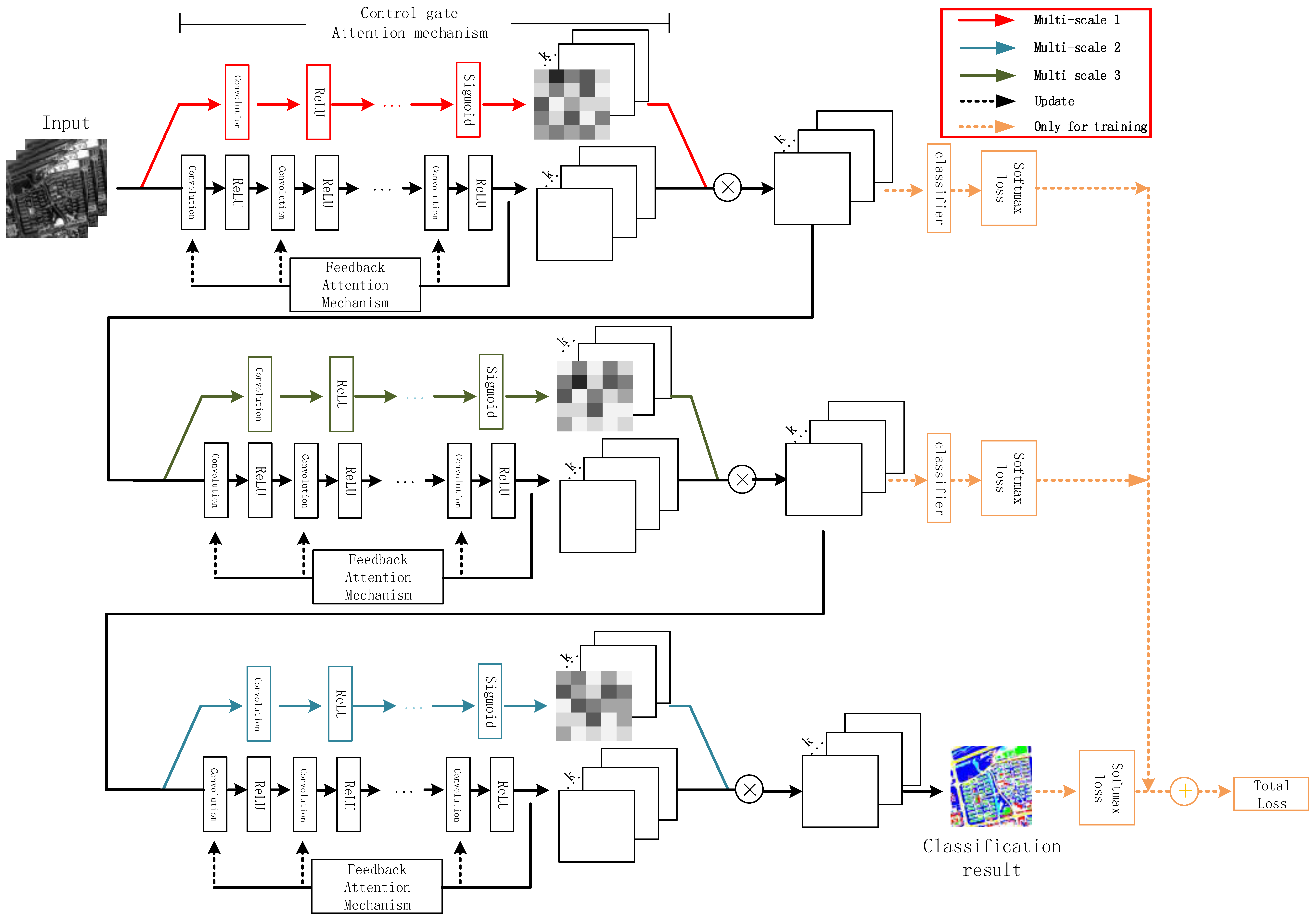
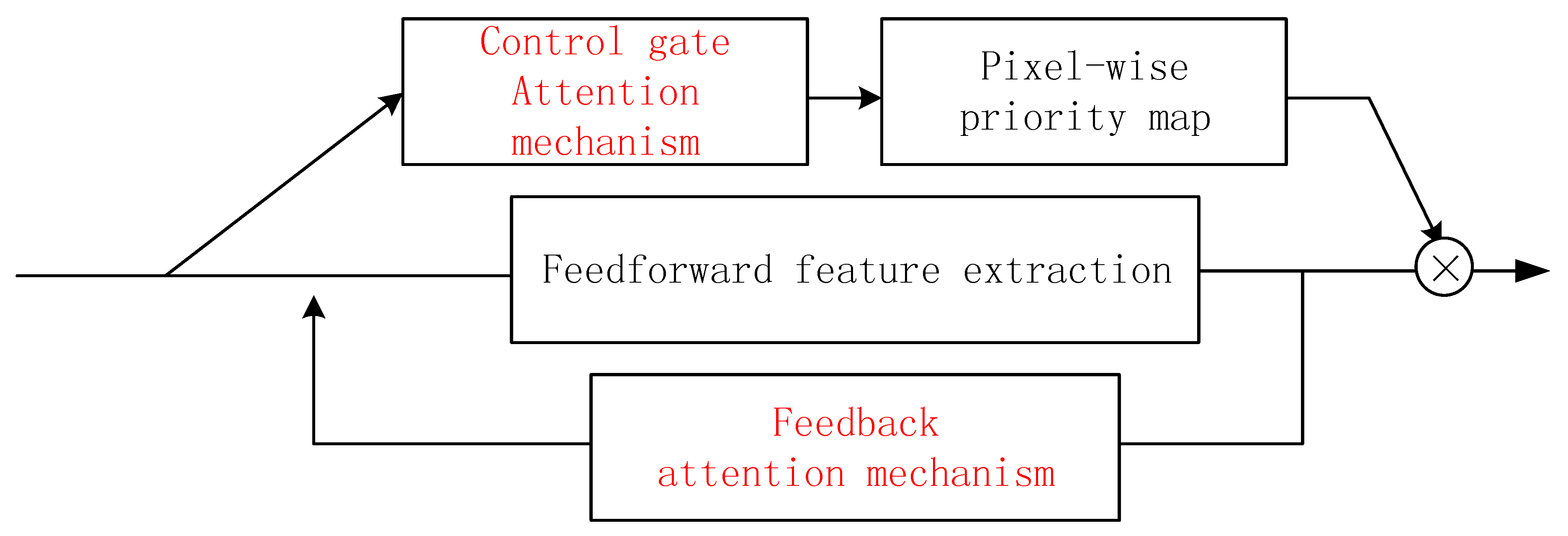
This section first introduces the mechanisms utilized in the framework and then presents the network construction. A flowchart of the attention-mechanism-based method is presented in Figure 1. The entire network is composed of several attention blocks. In each block, the soft attention mechanism and feedback attention mechanism form the control gate mask and trunk branches, respectively, and the point-wise multiplication of these two branches enables the fusion of these two attention mechanisms. Each block employs a control gate with a specified scale, and the stacking of the blocks allows the network to fuse the multi-scale information. The internal classifiers and softmax loss exist only for network training and are removed when the network is ready for image classification. The method is explained in detail below.

2.1. Feedback Attention Mechanism

Deep learning networks, such as the VGG neural network [12], ResNet [14], and DenseNet [35], all employ a feedforward approach to feature learning, in which high-level features are learned from low-level features. This hierarchical learning approach simulates the hierarchical structure of the images, in which points form lines, lines form graphs, graphs form parts, and parts form objects [25]. It has also been observed that humans can capture information on a target faster and with more precision when they re-consider the target with additional attention. 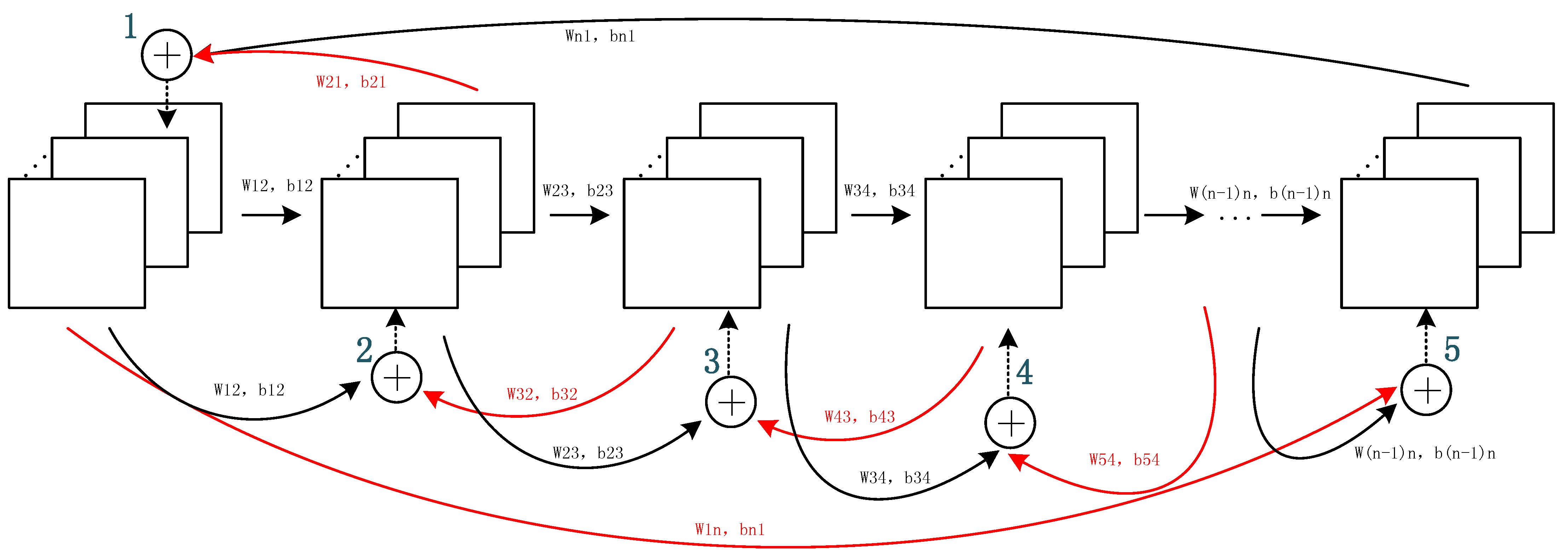Inspired by CliqueNet [29], we believe that the introduction of the feedback attention mechanism as a form of additional attention on high-level features can simulate this biological phenomenon, by assisting low-level feature learning for improved target-oriented feature extraction. In our design, the feedback attention mechanism comprises two parts: the feedforward and feedback stages. The feedforward stage learns high-level features from the low-level features acquired from the image details so as to acquire abstract and discriminative features. The feedback stage follows, in which high-level features are returned to aid lower-level feature learning. The convolutional network with the feedback attention mechanism is illustrated in Figure 2.

The feedforward process is a CNN without the classification layer. The CNN is an improved MLP, which is generated by several blocks stacked together, each of which is used for feature extraction and comprises convolution, pooling, and non-linear transformation.

The convolutional layer uses a sliding window as a kernel to move across the image and to calculate the point-to-point inner product in the corresponding area, such that each pixel in the features corresponds to a continuous area in the input data. This locally connected approach simulates the biological mechanism, in which a certain area in the visual cortex corresponds to some local area when information is transmitted to the human brain [42]. The kernel remains unchanged during sliding; hence, it performs image processing in a share weight manner for different locations. Share weights reduce the parameter amount between each pair of hidden layers and enable each kernel to locate similar features in the images at the same time. A greater number of kernels indicates more abundant feature representations, stronger feature mining ability, and more comprehensive extracted features.

The operation in the convolutional layer is a linear transformation that can handle the linearly separable problems. However, the features of a VHRRSI are complex, and cannot always be linearly simulated. Therefore, the introduction of non-linear layers is necessary to increase the network complexity and expression ability. In a CNN, such layers are called activation functions. Common activation functions include the rectified linear unit (ReLU), sigmoid, and tanh. Each function has its own advantages. In particular, the ReLU function, $\delta (x)=\max (0,x)$, assigns a 0 value to negative elements and maintains positive values. It reduces the training time [11], alleviates the gradient vanishing problem to some degree [43], and is a very widely used non-linear function.

The operation in the pooling layer is a statistical aggregation. This operation selects values to represent the corresponding and non-overlapping areas in the image, so as to reduce the feature map dimensions. Pooling increases the receptive fields and scale invariance of the features, reduces redundancy and computation, and retains the most representative features to help extract the hierarchical features. However, the pooling layer causes a loss of location information while increasing the receptive field. Moreover, the dimension reductions cause continuous changes in the feature map sizes, making it difficult to realize direct end-to-end and pixel-to-pixel image pixel-wise classification without up-sampling; this aspect increases the classification complexity. For this reason, dilated convolution [44] is used to replace pooling in order to increase the receptive fields, while also maintaining the spatial location information, keeping the feature maps of the same size as the input data, and realizing pixel-wise classification.

The dilated convolution flowchart is shown in Figure 3. Note that the kernel does not calculate the inner product in the continuous area on the feature map. The original kernel is expanded according to a skipping interval depending on the dilation size. The interval is filled with 0 values, meaning that the feature points at those locations on the kernel are not considered in the computation. The convolution is conducted between the expanded kernel and the feature map areas of the corresponding size; sample values are given in the flowchart to aid understanding. As the kernel expands, the area in the previous layers mapped by the nodes in the next hidden layer also expands, and the receptive field consequently expands. Through a padding operation, dilated convolution ensures that the generated feature maps are always the same size as the input data. This approach allows for the easy production of the final pixel-to-pixel, pixel-wise classification results.

The feedforward process is described in the following formula:

$$x_l=\delta \left(W_{l-1}\ast x_{l-1}+b_{l-1}\right)$$

where $\ast$ indicates the convolution operation; $x_{/}\in {\Re }^{s\times s\times n}$ represents the $n$ feature maps with size $s\times s$ generated by layer $l$; and $W_{/-1}$ is the set of various kernels used on the feature maps in layer $l-1$. Further, $W_{/-1}=\left(W_{/-1}{}^1,W_{/-1}{}^2,W_{/-1}{}^3,\dots ,W_{/-1}{}^n\right)$, where $W_{/-1}{}^n\in {\Re }^{w\times w\times k}$, indicating that the kernel size is $w\times w$ and its depth $k$ is equal to the third dimension of feature maps $x_{l-1}$ from layer $l-1$; $b_{l-1}$ is the bias corresponding to $W_{/-1}$; and $\delta \left(\right)$ is the activation function.

The aforementioned process is a hierarchical feature extraction that proceeds gradually from a low to high level. However, the features extracted at the high level do not provide additional assistance to the feature learning from the lower level. Therefore, in the proposed method, we add a feedback stage after the feedforward stage. This stage uses the features acquired in the high level to help re-weight the focus of the lower layer such that it assigns attention to the correct focus more quickly and effectively. The unrelated neuron activities that decrease the classification accuracy, including factors such as background information and noise, are simultaneously suppressed.

The feedback stage is also a CNN network (Figure 2). However, in this stage, the layers related to the feedforward stage are re-updated. All levels are re-updated by features acquired from one layer higher in the feedforward stage and one previous lower layer re-updated in the feedback stage. Apart from the first and last layers in the feedforward stages, all other stages are re-updated according to the following rule:

$$x_l=\delta \left(W_{l-1,l}\ast x_{l-1}+b_{l-1,l}+W_{l+1,l}\ast x_{l+1}+b_{l+1,l}\right)$$

where $W_{l-1,l}$ and $b_{l-1,l}$ are the local weight and bias from the hidden layer $l-1$ to layer $l$, respectively; $W_{l+1,l}$ and $b_{l+1,l}$ are the parameters bringing the higher-layer features from layer $l+1$ to layer $l$; and $\delta \left(\right)$ is the non-linear activation function.

Feature maps from layer $l$ are acquired by performing a convolutional non-linear transformation on the features from layers $l-1$ and $l+1$. In the feedback stage, the computation on the features from the higher and lower layer is performed element-wise, such that the dimensions of the kernels used for feature extraction and learning in all layers must remain the same in the feedforward process, along with the sizes of the generated feature maps. The last layer of the feedforward stage serves as the lower layer of the first layer in the feedback stage. Therefore, for the last layer of the feedback stage, the first layer can be considered as its higher layer.

In the feedback mechanism, parameters $W_{l-1,l}$ and $b_{l-1,l}$ are shared in the feedforward and feedback stages. Through the feedback of the higher layer and the feature combination with the low layer, feature reuse is realized to some degree. Under this condition, we can maximize the information flow. Meanwhile, because of the feature reuse, we can minimize the number of feature maps extracted from each layer to prevent information redundancy and the massive computational burden caused by high-dimensional kernels.

2.2. Control Gate Attention Mechanism

In addition to the aforementioned attention mechanism that returns the features from the higher layer to the lower layer to re-update the weight, we can also use the “control gate” to simulate the human focus mechanism. The human visual system is instantly attracted to important visual targets. This behavior indicates that the human visual system does not assign the same priority to different positions, but instead gives distinct priority to certain task-specific areas and features. In some studies, the priority assigned to certain pixels has been improved by increasing their weights. For instance, Pinheiro [45] aggregated the predicted pixel-wise labels to the image level and placed greater weights on pixels having corresponding image-level labels that matched the given image labels. However, transference of the pixel-level labels to the image-level labels seems a little complex. Therefore, in this study, we adopt an alternative method to adjust the priority, which is called the control gate approach.

A control gate allows for the focus and related resources to be assigned to the most intrinsic, discriminative, and informative areas. We use the control gate as a mask mechanism and utilize it for feature recalibration, selectively enlarging the valuable areas and suppressing useless features, such as noise and background. Unlike Hu et al. [28] and Yang et al. [29], who used global pooling to enlarge the valuable channels, our control gate performs pixel-to-pixel modeling on masks that are the same sizes as the original feature maps. The positions in the masks represent the weights or propriety values of the corresponding pixels on the original maps. The priorities of the pixels on the original feature maps can differ, indicating that each pixel may play a different role according to different classification objectives. These kinds of masks are more suitable for pixel-wise classification than global pooling.

The control gate is also a feedforward fully convolutional neural network that maintains the size of the acquired mask. The generated mask indicates the calibrated importance of every position on the feature maps; therefore, the control gate of the proposed method is designed as a soft attention mechanism, wherein the value of every pixel on the mask varies from 0 to 1 [27]. Therefore, the convolutional network of the control gate is also stacked using elements such as convolution and non-linear transformation. However, different from the feedback attention mechanism, we replaced the previously used ReLU non-linear transformation with the sigmoid activation function in the last layer of the control gate to ensure that the mask outputs are between 0 and 1. The sigmoid function is expressed as

$$\mathrm{S}\left(x\right)=\frac{1}{1+e^{-x}}$$

In this mechanism, the masks help recalibrate and select the most intrinsic and discriminative features toward the classification objective in the feedforward process, and also prevent the updating of the parameters with incorrect gradients during backpropagation [20]. Therefore, the use of such a control gate mechanism renders our network more expressive and robust.

2.3. Structure of the Proposed Method

As the attention mechanism can be beneficial for pixel-wise classification, in this study, we build a multi-scale deep neural network that fuses two different attention mechanisms: soft and feedback.

2.3.1. Fusion of Two Attention Mechanisms

The two attention mechanisms have different objectives; hence, we take these two mechanisms as different components to form the framework. The fusion of the two mechanisms is shown in Figure 4.

The feedback attention mechanism is designed to form the trunk branch, so as to handle attention-aware feature learning. The trunk branch has two stages; in the first, the higher-layer features are learned from the low level in a bottom-up manner to implement hierarchical feature learning. In the feedback stage, all the layers are re-updated with one layer higher and one layer lower information using the top-down strategy. Hence, both shallower and deeper information are fused to help re-weight the focus and train the network in a more task-oriented manner. In short, the trunk branch implements a feature re-use and focus re-weighting process.

The control gate is not utilized for feature extraction, but rather to learn the weights corresponding to the features’ importance in the feature extraction process. Therefore, the control gate serves as a mask branch to assist the feedback-attention-based trunk branch, rather than the main stream.

In many previous studies, such as that by Wang et al. [20], down- and up-sampling were used to reduce and restore the mask dimensions when constructing mask branches. This approach enlarges the receptive field while generating masks of the same size as the input data. However, this method inevitably yields information loss. Therefore, in the proposed method, we use dilated convolution to replace the pooling for receptive field enlargement when constructing the convolution networks for the trunk and mask branches. The sizes of the generated feature maps and the mask maps remain unchanged from the original input data, which is convenient for the soft attention mechanism and the pixel-to-pixel and end-to-end pixel-wise classification.

The feature maps and mask maps from the trunk and mask branches, respectively, are fused by implementing element-wise multiplication on the corresponding positions. Hence, the extracted features are recalibrated according to their weights, such that different priorities are assigned to pixels at different locations and on different channels. As a result, more goal-oriented, effective, and discriminative features of ground objects are acquired for pixel-wise classification.

2.3.2. Stacking of Multi-Scale Attention-Mechanism-Containing Modules

A deep network constantly receives feature maps from different layers, and these maps represent different and hierarchical features; hence, different attention mask branches are required to acquire different focuses and to combine them to handle complex ground conditions. Therefore, the trunk and attention branches are fused into a module, and multiple module stacking is used to model the requirements for different focuses. The recalibrated feature maps from the previous module are input to the next module as input data for the next feature learning and recalibration. The constantly added attention modules enable us to acquire different kinds of attention focuses and, therefore, increase the expressive capacity of the network [20].

In accordance with the characteristics of the deep network, increasing the network layer depth causes the feature maps extracted by the network to change hierarchically. Therefore, when the network is stacked using several modules, the shallow modules extract features with a greater focus on detailed information such as boundaries and locations, while the features from the higher modules are more abstract, discriminative, and target-oriented. The control gates must be adjusted according to the feature map type because the characteristics of the extracted features differ. Therefore, the control gate spatiality can be adjusted so that it fits the characteristics of the hierarchical features. From shallow to deep, different modules are equipped with masks using different convolution kernels of varying sizes, which focus on different local spatial structures. Kernels with a size of 1 × 1 focus on the pixels themselves and the relationships among the bands; therefore, they are better suited to processing details-focused feature maps. In contrast, kernels of larger sizes generate larger receptive fields, and the focus is on the surrounding spatial structures. More global information is considered; therefore, these kernels are more suitable for handling the abstract features generated by higher modules. Additionally, the receptive fields of feature maps generated by deeper layers are bigger, which correspond to an improved matching. Another benefit of using kernels of different sizes is that spatial and spectral joint features can be utilized because small kernels place greater focus on spectral information, whereas larger kernels concentrate on spectral and spatial information. Ground-object classification can be difficult if we rely solely on spectral information for classification because of the uncontrolled field conditions for ground objects with similar spectra. However, if we rely solely on spatial information, the intrinsic information provided by the spectral information may be ignored.

Module stacking continuously increases the network length. Although increased depth is a research trend in the field of neural networks, problems such as gradient vanishing and training difficulty render the network capability disproportionate to the network depth. Huang et al. [35] believe that shorter connections between the input and output layers can lower the risks associated with a deeper network. Motivated by past research [40,46,47], in this study, we construct supervised learning by implementing additional supervisions for each module and then by combining their loss with that of the top classifier. In this manner, gradients can be propagated to shallow layers more efficiently during backpropagation, which is more convenient for network training and optimization. Meanwhile, when classification results generated by different-scale modules are improved in the direction of the ground truth, internal classifiers enhance the hidden-layer transparency and the features are extracted in the target-oriented direction. This approach reduces the feature redundancy and improves the feature extraction efficiency.

The outputs of the internal classifiers and the final top classifier are all pixel-to-pixel classification results of multiple categories. The difference between the output results and ground truth results is called Loss. We define the Loss function for each classifier as

$$\mathrm{Loss}(\mathsf{\theta })=-\frac{1}{M\times N}\left[{\displaystyle {\sum }_{m=1}^M{\displaystyle {\sum }_{n=1}^N{\displaystyle {\sum }_{c=1}^{C}1\{y^{(m,n)}=c\}}}}\log \frac{\exp (p_{m,n}^c)}{{\displaystyle {\sum }_{k=1}^K\exp (p_{m,n}^k)}}\right]+\frac{\lambda }{2}{\Vert \mathsf{\theta }\Vert }^2$$

The classifier generates a pixel-wise classification result with size $M\times N$. Here, $y^{m,n}$ is the class of the pixel at location $\left(m,n\right)$ in the classification result. Every pixel can be classified into one of $C$ types. Further, $\mathsf{\theta }$ is the network parameter and $p_{m,n}^k$ is the probability of the pixel at location $\left(m,n\right)$ on the original image being classified as type $k$. Finally, $1\left\{\right\}$ is the indicative function: if the equation in brackets is true, the function returns 1; otherwise, it returns 0. Therefore, the overall cost function of the network is as follows:

$$\mathrm{Cost}={\displaystyle {\sum }_{l=1}^L{\mathrm{Loss}}^l}$$

where $\mathrm{Cost}$ indicates that, in the pixel-wise classification, the total Loss generated by the network comprises the Loss from different scale modules and the Loss from the top of the network. $L$ is the total number of modules. With supervision on all modules, the network performs training in a more robust and effective manner and, consequently, achieves superior classification results. The acquired $\mathrm{Cost}$ is used in the backpropagation to update the network parameters.

Therefore, the overall training workflow is as follows: the image data are input to the network, after which they pass through the modules in sequence. Each module uses the control gate with different scales to observe, acquire, and highlight the attention-aware features of the feature maps. In each module, the input data are processed in the trunk and mask branches. When the feature and mask maps are generated, the mask maps are utilized to recalibrate the feature maps through element-wise multiplication. Hence, different priorities are assigned to the different areas of the input data, and consequently, useful features are highlighted while unnecessary features such as noise and background are suppressed. Then, internal classifiers are used to conduct pixel-wise classifications of the feature maps generated by the previous modules, and the results and ground truth are compared to calculate Loss. The features for internal classifiers are also inputted into the module of the next scale for consequent feature extraction. The final classification result fused with the loss functions from previous modules is utilized to update the network iteratively.

3. Experiments and Results

3.1. Experiment Setup

In this section, the experiment setup is described, including the data preparation and experiment strategies.

3.1.1. Experimental Data

All experimental data utilized to test our proposed method were obtained from datasets shared by other researchers and their work [40,48]. We used 20 images in total and the data were collected from four satellites. All images are displayed in Figure 5.

Fourteen images were obtained from the GaoFen-2 (GF02) satellite, having sizes varying from 600 × 600 to 950 × 950. The GF02 images are panchromatic with a 1-m spatial resolution; with red, green, blue, and near-infrared bands; and with 4-m spatial resolution. The images used in this study were acquired on the 25 June 2016, over Dongying City, Shandong Province, China. Five categories were labeled on the images: residential areas, water bodies, vegetation, road, and bare land.

Four images were obtained from the Beijing-2 (BJ02) satellite, having sizes varying from 400 × 400 to 950 × 950. Images from the BJ02 satellite also possess five panchromatic bands with a 1-m resolution and four multi-spectral bands with a 4-m resolution. The images used in this study were taken over Dongying City, Shandong Province, China, on 21 June 2017. Five or six classes could be observed on this dataset: residential areas, parking areas, water, vegetation, road, and bare land.

One image was acquired from the Quickbird satellite, which was taken over Fancun, Hainan Province, China, in 2010. This satellite provides a 2.4-m spatial resolution for the red, blue, green, and near-infrared bands. The image was 400 × 400 in size with five marked categories identical to those on the GF02 satellite images.

One image was acquired from the Geoeye satellite, which was taken over the urban area of Hobart in Tasmania, Australia, in September 2012. This satellite provides a 0.5-m spatial resolution for the red, blue, green, and near-infrared bands. The image was 600 × 600 in size with six labeled categories: residential areas, grass, water, trees, roads, and bare land.

For pixel-wise classification, which is a form of pixel-to-pixel classification, the proposed method was tested by randomly selecting a small proportion of the pixels as training samples, with the others being retained for testing. The training samples were acquired as follows. For each image, $m$ bands were stacked first. If the training ratio was $p\%$ and the number of pixels with ground truth labels was $n$ in total, $n\times p\%$ pixels were randomly selected from the image. For each selected pixel, one patch $x$ of size $w\times w\times m$ around that pixel was acquired from the image. The location for that pixel on the patch was randomly selected and that location was recorded. Each patch’s corresponding ground truth data $y$ was of the same size as the patch $x$. Only the recorded location on $y$ was viewed as labeled for Loss calculation and backpropagation, while the others were labeled as “0”, viewed as background, and were not considered in the calculations. Accordingly, we can guarantee that, for every pixel on $x$, there would be a one-to-one correspondence on $y$. All data were normalized by dividing by 255 and subtracting the mean value to remove the effects of different conditions caused by illumination and so on. No other pre-processing was required.

3.1.2. Experimental Strategy

We chose one image from each of the BJ02 and GF02 datasets for the main experiments. The images included five and six kinds of ground objects, respectively, and the detailed results of the comparative analyses are presented here. The detailed label information is presented in

Table 1. The reference data information for the Bei-Jing02 and Gao-FenF02 images.

BJ	Size 800 × 800
No.	Category	Mark Color	Number of Pixels
1	Water	Light Blue	35,522
2	Tree	Blue	226,305
4	Bare Land	Red	70,549
5	Building	Green	115,512
6	Road	Yellow	71,464
GF	Size 600 × 600
No.	Category	Mark Color	Number of Pixels
1	Water	Light Blue	32,206
2	Tree	Blue	97,121
4	Bare Land	Red	51,160
5	Building	Green	75,393
6	Road	Yellow	28,038
7	Car	Purple	13,115

.

We used a variety of network structures to conduct pixel-wise classification experiments. The proposed neural network is stacked with modules; hence, the number of modules determines the network length. To verify the influence of the network length on the pixel-wise classification results in the experiments, we tested networks consisting of 1, 2, and 3 modules, each of which contained five convolutional blocks. For the shallow module in the network, we used 1 × 1 convolutional kernels to construct the control gate. Through the module stacking, the sizes of the convolutional kernels used to construct the mask branch gradually increased, and the mask branch acquired different attention focus points from the hierarchical feature maps. This behavior confirmed the influence of the combination of different attention mechanisms on the network expressive ability.

The number of convolutional kernels in the network determines the number of feature maps extracted by the network; thus, it determines the expressive ability of the network to some degree. More convolutional kernels correspond to the extraction of more abundant features by the network. However, increased numbers of convolutional kernels are disadvantageous with regards to the computational burden, information redundancy, etc. Some studies [35,40] utilizing feature fusion and concatenation have proven that a kernel depth as shallow as 12, 24, or some other low value could still be effective because of the feature reuse. As the fusion of features from different layers occurs in our trunk branch, a moderate number of convolutional kernels were used in this study. In detail, we used the convolutional kernel settings of 14, 18, 22, 26, and 30 to examine the influence of the number of convolution kernels on the network and to examine the influence of the network structure on the network performance.

We analyzed the influence of the number of training samples on the network for different network settings. For remote sensing images, the acquisition of a large volume of labeled training data is difficult. Therefore, good performance with a small volume of sample data is a good achievement. For networks with different lengths and numbers of convolutional kernels, we tested the network performance with the labeled training pixels from the 300 pixels/category to the 700 pixels/category and examined the influence of the training data volume on the different network configurations.

To prove the rationality and effectiveness of the network components, we discussed the influence of the network components on the network performance. We compared the proposed method with networks without internal classifiers, without the control gate attention mechanism (the mask branch), and without the feedback attention mechanism, so as to investigate the importance of those components to the network.

Besides the detailed investigations conducted in the two main experiments described above, we also compared our method with state-of-the-art methods. The proposed method was also applied to another 10 images to verify its stability and effectiveness

In all the experiments, we set the training sample size to 35 × 35. This was a tradeoff between the computational cost and experimental efficacy. To combine both spatial and structure information, we employed kernels with three different sizes: 1 × 1, 3 × 3, and 5 × 5. When the 1 × 1 kernels were applied to each band, the emphasis was on the spectral coherence between different channels. With reference to a previous study [12] and considering the input data size and number of parameters to be trained, the 3 × 3 and 5 × 5 kernels were also selected. With regards to the convolution step, a stride s = 1 was proven effective in previous works [25,49] and was therefore employed in this study. The padding for each side was set to 0, 1, and 2 for the 1 × 1, 3 × 3, and 5 × 5 kernel sizes, respectively, to ensure that the feature map sizes remained unchanged during the convolution process. As the input patches adopted for the experiments were relatively small and the receptive field generated by a dilated value of 2 could already satisfy the requirements of our input patches, the dilated value was set to 2. Following previous research methods [12,43], we set the batch size in the deep network training to 150, the learning rate to 0.004, the weight decay to 0.0005, and the momentum to 0.9. The network configuration for a kernel depth of 30 is presented in

Table 2. The network configuration for kernel depth of 30.

Operation			Kernel Dimension			Output (with Padding)
Input			\			35 × 35 × 3
Convolution			3 × 3 × 3 × 30			35 × 35 × 30
			Module 1	Module 2	Module 1
Trunk branch	feedforward Block 1–5	convolution	3 × 3 × 30 × 30	3 × 3 × 30 × 30	3 × 3 × 30 × 30	35 × 35 × 30
		Non-linearity	\	\	\	35 × 35 × 30
	Feedback Update 1–5	convolution	3 × 3 × 30 × 30	3 × 3 × 30 × 30	3 × 3 × 30 × 30	35 × 35 × 30
		convolution	3 × 3 × 30 × 30	3 × 3 × 30 × 30	3 × 3 × 30 × 30	35 × 35 × 30
		fusion	\	\	\	35 × 35 × 30
		Non-linearity	\	\	\	35 × 35 × 30
Mask branch	Feedforward	convolution	1 × 1 × 30 × 30	3 × 3 × 30 × 30	5 × 5 × 30 × 30	35 × 35 × 30
		Non-linearity	\	\	\	35 × 35 × 30
		convolution	1 × 1 × 30 × 30	3 × 3 × 30 × 3	5 × 5 × 30 × 30	35 × 35 × 30
		Non-linearity	\	\	\	35 × 35 × 30
		convolution	1 × 1 × 30 × 30	3 × 3 × 30 × 3	5 × 5 × 30 × 30	35 × 35 × 30
		Non-linearity	\	\	\	35 × 35 × 30
Fusion	Element-wise multiplication		\	\	\	35 × 35 × 30
Classification	convolution		3 × 3 × 30 × C	3 × 3 × 30 × C	3 × 3 × 30 × C	35 × 35 × C
	Softmax		\	\	\	35 × 35 × 1

, as an example.

For each group of experiments, we used the average results of five experiments to guarantee fairness. Within each round, the training samples were randomly reselected according to our data preparation strategy. All experiments were conducted on a computer with a 16.0 GB RAM Intel^® Xeon^® CPU [email protected] GHz processor. The computer featured an NVIDIA Quadro K620 graphic card with CUDA version 8.0.4 for acceleration.

3.2. Experiment Results

3.2.1. Analysis of Experiment Results

In the two main experiments involving BJ02 and GF02, we used multiple network settings to test the proposed method. As evaluation standards, we used the overall accuracy (OA) and Kappa, the most widely adopted criteria in remote sensing image classification accuracy assessment. The accuracies of the pixel-wise classification for BJ02 and GF02, which were acquired using various numbers of modules and convolution kernel depths under a training data ratio of 700 pixels/category, are shown in Figure 6 and Figure 7, respectively. The detailed OA and Kappa results are presented in

Table 3. The OA values for the BJ02 images.

	1 Subnet	2 Subnets	3 Subnets
14	0.9667	0.9685	0.9729
18	0.9678	0.9707	0.9746
22	0.9700	0.9715	0.9762
26	0.9705	0.9732	0.9771
30	0.9700	0.9760	0.9791

,

Table 4. The Kappa values for the BJ02 images.

	1 Subnet	2 Subnets	3 Subnets
14	0.9446	0.9476	0.9550
18	0.9463	0.9513	0.9577
22	0.9501	0.9526	0.9603
26	0.9508	0.9554	0.9619
30	0.9502	0.9600	0.9652

,

Table 5. The OA values for the GF02 images.

	1 Subnet	2 Subnets	3 Subnets
14	0.97558	0.9808	0.9808225
18	0.97619	0.981852	0.982748
22	0.977705	0.983234	0.98445
26	0.97801	0.98442	0.9856
30	0.97859	0.985548	0.987125

and

Table 6. The Kappa values for the GF02 images.

	1 Subnet	2 Subnets	3 Subnets
14	0.96696	0.9740	0.9740
18	0.9677	0.9754	0.9766
22	0.9697575	0.9772	0.9789
26	0.97019	0.9789	0.9805
30	0.97094	0.9804	0.9825

. Furthermore, the producer and user accuracies, which are forms of commission and omission errors, are given for each category in

Table 7. The BJ02 classification results for all comparative experiments. The producer (x) and user (y) accuracy results are presented in the x/y form.

Method	OA	KAPPA	Water	Tree	Bare Land	Building	Road
Proposed method	0.979	0.965	0.997/0.936	0.982/0.999	0.959/0.927	0.973/0.971	0.984/0.953
Non-internal classifier	0.966	0.945	0.996/0.924	0.970/0.998	0.950/0.865	0.951/0.957	0.973/0.934
Without feedback stage	0.958	0.930	0.996/0.889	0.965/0.997	0.925/0.860	0.933/0.948	0.971/0.889
Without mask attention	0.972	0.953	0.998/0.916	0.980/0.998	0.945/0.892	0.947/0.962	0.974/0.942
CNN	0.945	0.910	0.996/0.898	0.956/0.998	0.895/0.843	0.915/0.906	0.954/0.848
Contextual CNN	0.967	0.944	0.994/0.957	0.985/0.998	0.937/0.858	0.911/0.959	0.961/0.919
DenseNet	0.970	0.950	0.996/0.932	0.985/0.999	0.920/0.896	0.930/0.956	0.981/0.919
URDNN	0.964	0.940	0.994/0.901	0.971/0.998	0.926/0.909	0.950/0.930	0.965/0.909
DNN	0.962	0.937	0.990/0.918	0.976/0.998	0.927/0.850	0.929/0.938	0.959/0.940
SCAE + SVM	0.888	0.817	0.868/0.756	0.960/0.995	0.804/0.752	0.746/0.744	0.788/0.738
SENet	0.969	0.948	0.993/0.965	0.982/0.997	0.952/0.879	0.926/0.952	0.965/0.930

and

Table 8. The GF02 classification results for all comparative experiments. The producer (x) and user (y) accuracy results are presented in the x/y form.

Method	OA	KAPPA	Water	Tree	Bare Land	Building	Road	Car
Proposed method	0.987	0.983	1.000/0.993	0.990/0.996	0.975/0.967	0.984/0.993	0.995/0.984	1.000/0.940
No-internal classifier	0.977	0.970	0.998/0.996	0.976/0.997	0.973/0.936	0.970/0.980	0.995/0.965	0.999/0.919
Without feedback	0.975	0.966	0.998/0.994	0.976/0.996	0.978/0.919	0.959/0.987	0.993/0.969	1.000/0.887
Without mask	0.982	0.976	0.999/0.994	0.982/0.996	0.976/0.948	0.976/0.985	0.994/0.983	0.999/0.927
CNN	0.974	0.964	0.995/0.993	0.979/0.994	0.969/0.920	0.955/0.985	0.992/0.963	0.999/0.877
Contextual CNN	0.974	0.964	0.998/1.000	0.987/0.997	0.983/0.895	0.932/0.989	0.990/0.954	0.997/0.954
DenseNet	0.976	0.968	1.000/0.999	0.982/0.999	0.977/0.907	0.956/0.991	0.984/0.952	0.997/0.959
URDNN	0.972	0.962	0.999/0.999	0.966/0.990	0.972/0.911	0.968/0.991	0.978/0.923	0.991/0.959
DNN	0.968	0.956	0.999/0.993	0.958/0.989	0.953/0.907	0.973/0.982	0.988/0.930	0.998/0.936
SCAE + SVM	0.919	0.892	0.991/0.861	0.963/0.994	0.881/0.876	0.892/0.957	0.988/0.679	0.442/0.909
SENet	0.977	0.969	0.998/0.993	0.976/0.995	0.972/0.949	0.970/0.986	0.991/0.906	0.997/0.968

.

The evaluation results for the BJ02 images are shown in Figure 6. For these images, the proposed method achieved classification results with an accuracy exceeding 97.9%. From the experimental results, we found several trends in the accuracy variation. In most cases, although the networks featured different depths, an increase in the number of convolutional kernels strengthened the network classification ability. This was because each convolutional kernel represented a certain kind of feature on the image. With an increase in the number of convolutional kernels, the number of feature maps generated by the relevant feature detectors also increased. Hence, the features extracted by the networks were more comprehensive. This enabled the networks to analyze the different ground objects in the images from different angles and to find the intrinsic differences among the different ground objects to perform the classification. Although we used low kernel depths in the experiments (compared with the 128 kernels more commonly employed in other networks), and the kernel depths only varied from 14 to 30 with intervals of 4, the accuracy increase was discernible. This result was obtained because we use feedback attention in our network, which returned the high-level features to the lower level and fused the features from different layers to re-weight the focus. Therefore, although we used convolutional kernels with low depths, through feature fusion, the number of features involved in the feature learning for each layer was twice the kernel depth used at the corresponding layer. Thus, the network achieved good accuracy.

Besides the kernel depth, networks with different depths also yielded different results. For the 700 pixels/category training data ratio, the 3-module network, which was the deepest network, exhibited the best performance. The network performance was in direct proportion to the network depth. A deeper network is always considered to have better expression ability. It is expected to extract more and richer hierarchical features, from detailed to abstract and from general to class specific, whereas the features obtained from a shallow network may have a poorer sense of hierarchy. In this study, the deeper networks were equipped with attention masks at different scales, not only considering the spectral information, but also the different local spatial structures. As a result, more attention points were combined to handle the complex classification conditions. Furthermore, for the shallow networks and, in particular, the 1-module network, the accuracy changes with increased kernel depth tended to be stable, while the accuracies for the 2- or 3-module network still displayed a growth tendency. Although the use of more kernels could yield more inherent and discriminative features from different angles, which would help improve the network expression ability, the accompanying benefits could be limited by the network depth. Only by using the combined effects of the network and kernel depths can we fully develop their individual advantages. The above results indicate that the network structure is significant for modulating its performance.

The experimental results for the GF02 images are shown in Figure 7. Although these images had one more category compared with the BJ02 images, the obtained trends are very similar to those observed in the experiments on the BJ02 images. Within the ambit of the experimental setup of this study, the OA and Kappa of the network showed an increasing trend when the number of convolutional kernels increased. This indicated that an increase in the number of convolution kernels enhanced the network feature extraction angles and allowed the networks to describe ground objects more comprehensively. Without greatly increasing the number of parameters to be trained, the network performance can be improved to a certain extent. In addition, although the accuracies acquired for the 2-module network were very close to those for the 3-module network, the deepest network exhibited the best performance and yielded an OA as high as 98.7%. Finally, for the shallower network, the changes induced by changes in the kernel depth seemed smaller than those generated by the deeper network. This finding proved the significance of the network depth once more and revealed the trend that more features can induce more effects with the cooperation of the network’s hierarchical characteristics.

3.2.2. Network Component Influences on Network Performance

In Section 2, we illustrated the network design in detail and analyzed the rationality of the network in theory. In this section, we demonstrate the influence of every network component by analyzing and comparing the result accuracies for networks with different components. Hence, the rationality of the network design is verified.

In this part of the study, we used a network with a fixed length (three modules), a fixed number of convolution kernels (30 kernels), and a fixed training data volume (700 pixels/category), to compare the proposed method with networks without internal classifiers, without mask attention, and without feedback attention. Other than the aforementioned parameters, all other parameters, such as the learning rate and batch size, were the same.

Influence of Internal Classifiers

Internal classifiers are classifiers added to the end of each module. They aid the application of the extracted features for the classification and comparison of the classification results with the ground truth. They also serve as the companion loss to aid the top classifier in training the network in a supervised manner. The results for the network with internal classifiers removed are displayed in Figure 8 and Table 7.

For the BJ02 image, the accuracy decreased by 1.3% after the internal classifiers were removed, the OA decreased from 97.9% to 96.6%, and Kappa declined from 96.5% to 94.5%. These results may be related to the fact that the internal classifiers enhanced the hidden layers’ transparency. The direct use of feature maps obtained by hidden layers for classification can promote the effectiveness of the extracted features and reduce the feature redundancy to some degree. Furthermore, the internal classifiers allowed the loss to be propagated to the shallow layers directly, which improves the convenience and efficiency of the backpropagation training. Without internal classifiers, the network can depend on the top (final) classifier only to conduct supervised learning. Thus, the hidden layer feature extraction capability will not be enhanced, yielding a decrease in the network classification performance.

When viewing the pixel-wise classification result map, it should be noted that most ground objects were successfully kept intact and the house edges were clear. However, there were a few sporadic and miscellaneous classification errors inside the vegetation area, which degraded the object integrity. Furthermore, some confusion between roads, bare land, and buildings occurred; for instance, some pixels inside or on the edges of the roads were apparently misclassified as bare land, and a similar situation occurred inside the buildings. This may have happened because these three kinds of ground objects contain artificial components, and some of the building materials exhibit very similar spectral characteristics or texture features, which would have caused confusion. Although misclassification between bare land and buildings also occurred when the proposed method was used, in general, there was no confusion for large areas, and the ground object edges (especially the house, road, and vegetation edges) were better preserved; consequently, the object integrity was improved.

For the GF02 image, the OA and Kappa both declined by 1% compared with the results obtained using a complete network, yielding OA = 97.7% and Kappa = 97.0%. Compared with the proposed method, some small objects were easily confused with some other objects. However, most of the ground objects (especially the building edges) were well preserved, the integrity of the object interior was relatively high, and the mapping accuracy and user accuracy were relatively balanced. Therefore, no obvious or large-area confusion occurred.

Influence of Attention Mechanism

Two types of attention mechanisms are involved in the framework of the proposed method: the control gate attention mechanism serving as the mask branch and the feedback attention mechanism playing a role in the trunk branch. The former assigns different weights to pixels from different positions according to their importance and distinct priority. Thus, it directs attention towards the most informative areas that help improve the network classification capability. The feedback attention mechanism returns higher-level features to the lower layers to re-weight the focus and re-update the feature learning, causing the network to re-learn the weights in an objected-oriented manner.

In this part of the study, we compared the proposed method with frameworks employing the same network structure, but with the mask branch and feedback stage removed.

One BJ02 image was considered here, and the OA and Kappa results are presented in Figure 8 and Table 7. When the control gate attention mechanism was removed, relatively good results were achieved, with OA reaching 97.1% and Kappa reaching 95.2%. This was despite the fact that the accuracies were lower than those from the proposed method. In contrast, when the feedback attention mechanism was removed, the accuracy decrease was more obvious. The OA was only 95.7% and Kappa declined by 3.5%. When both attention mechanisms were removed, the network became an ordinary CNN network; the OA decreased to 94.5% and Kappa declined to 91% when the other conditions remained the same. The results verified that the combination of the two attention mechanisms can greatly improve the network classification ability.

Considering the visual effects for pixel-wise classification result maps, we found that the resulting maps appeared to be more mottled when both attention mechanisms were removed. In addition, obvious errors were detected in the dense residential area to the right side of the image. The building edges were confused with bare land, and massive bare land areas were found on the edges or inside the roads. Furthermore, several speckled buildings and bare land areas were also found inside the vegetation. In comparison, the resulting map generated by the proposed method seemed to be clearer and had better visual effects. Some confusion remained on the edges or inside objects, but the ground object integrity was much higher.

The results of the GF02 experiment are presented in Figure 9 and Table 8. Hence, it is apparent that removing the two attention mechanisms affected the classification results, particularly when the feedback attention mechanism was omitted. This was reflected in the apparent decrease in the network classification performance, with the OA decreasing to 97.5% and Kappa decreasing to 96.6%. The pixel-wise classification result maps revealed obvious misclassifications inside the objects on the upper right, along with misclassifications between the bare land, trees, and buildings inside the bare land region on the left side. When the proposed method was compared with the conventional CNN (with both attention mechanisms removed), the results generated by the conventional CNN were more mottled. The bare land inside the parking lot was totally misclassified as cars, and the confusion between the cars and roads was more significant for the conventional CNN than the proposed method.

Both the precision results and the visual effects proved that fusion of the two attention mechanisms can improve the network capability of the conventional CNN, and help achieve superior classification. Compared with the conventional CNN, mask branches with different scales can help the network acquire different focuses of attention. Hence, the network may acquire distinct spatial structure information on different scales. Utilizing such operations can help highlight the most important or informative features on the current scale, facilitating the suppression of information that decreases the classification accuracy, such as background noise. Furthermore, a multi-scale mask branch does not only limit classification to the object spectral information, but also considers the environment surrounding the objects. Accordingly, although similar spectral information may exist among some artificial objects, the misclassification generated by the proposed method is less pronounced than that of the other methods considered herein. In addition, the feedback attention mechanism incorporated in the proposed method increases the feature re-use efficacy of the network compared to the conventional CNN. Furthermore, attaching additional attention to high-level features can help the lower level to re-update the feature learning direction and train the network toward the goal. The network re-weights the focuses based on the acquired features and captures the most discriminative and inherent features associated with the classification targets more quickly and effectively. Hence, with the help of the two incorporated attention mechanisms, the proposed method achieved an improved accuracy, reduced noise in the classification result maps, and an improved object and edge integrity in these experiments.

3.2.3. Comparison with other Methods

To verify the proposed method, we compared it with various state-of-the-art methods. The methods used for comparison in this part of the study were the deconvolutional neural network (DNN) [43], the unsupervised-restricted DNN (URDNN) [42], SENet [28], the contextual deep CNN [39], DenseNet [40], and SCAE + SVM [50]. Note that the first three methods are all neural networks with an attention mechanism.

DNN [43] and URDNN [42] both utilize the bottom-up and top-down feedforward attention mechanisms. They employ convolution and deconvolution to realize end-to-end and pixel-to-pixel pixel-wise classification. In this experiment, after multiple-round tests, the DNN and URDNN methods yielded superior results when three convolution-deconvolution stages and 3 × 3 × 64 convolution kernels were used. The adopted pooling and unpooling size were 2 × 2. The learning rate was set to 0.005, the batch size to 100, the momentum to 0.9, and the weight decay to 0.0005.

SENet [28] uses an attention mechanism that recalibrates features by utilizing the global information as the mask branch in order to enlarge the valuable channels. SENet was originally designed for scene classification; therefore, we adjusted it slightly in this experiment, so that it was suitable for pixel-wise classification. To facilitate comparison with the other techniques, the adopted SENet involved three residual blocks, with three convolution layers being utilized for each block. Here, the 1 × 1 and 3 × 3 kernels were used inside each residual block. Three masks were adopted, corresponding to the number of residual blocks. Each mask contained one global pooling layer using a 1 × 1 × C kernel (C was set to 30 here), two fully connected (FC) layers using a 1 × 1 × C kernel, and one sigmoid layer using a 1 × 1 × C kernel. The learning rate was set to 0.003, the weight decay to 0.0005, and the momentum to 0.9.

Contextual deep CNN [39] is a multi-scale network based on ResNet. Note that ResNet has achieved excellent results for the gradient vanishing problem. For multi-scale feature extraction, three kinds of convolution kernel were utilized for the first convolution layer: 1 × 1, 3 × 3, and 5 × 5. For the remainder, only 1 × 1 kernels were used and eight convolution layers were equipped, followed by one softmax layer. The kernel depth was set to 32 after several rounds of experiments. The momentum was 0.9, the weight decay was 0.0005, and gamma was 0.1. The learning rate started at 0.001.

DenseNet [40] is a neural network based on feature union and reuse, which concatenates features from different layers to extract the features of higher layers. This method involves feature fusion of different layers, similar to the proposed method, but utilizes the feedforward union only, whereas the proposed method uses the feedback form. After several rounds of testing, the best results for DenseNet were obtained using the settings provided in the literature [40].

SCAE + SVM [50] is the only unsupervised network for feature extraction in the six compared methods. It uses image reconstruction for feature extraction, and then uses the SVM classifier for classification. After several rounds of testing, it was decided to adopt three encoder-decoder blocks for SCAE. For internal convolution and convolution transform, the kernel size was set to 3 × 3 × 64. The adopted pooling and up-sampling size were 2 × 2. The learning rate was set to 0.005, the batch size to 100, the momentum to 0.9, and the weight decay to 0.0005. For SVM training, the radial basis function (RBF) kernel was used and training was performed in A Library for Support Vector Machines (LIBSVM).

All accuracies and images of the classification results are presented in Figure 8 and Table 7. Besides OA and Kappa, the accuracies of each ground-object category are also indicated by the producer (x) and user (y) accuracies, which are presented in the x/y form.

For the BJ02 images, of the three methods utilizing the attention mechanism, SENet achieved the best classification accuracy at 96.9%. However, compared with the proposed method, the OA was more than 1% lower, and the Kappa coefficient was approximately 2% lower. With regards to the visual effect, the integrity and boundary preservation exhibited by the considered methods was inferior to that of the proposed method. We believe that this is related to the attention mechanism used in those techniques. SENet implements the control gate attention mechanism, which is also used in our proposed network. However, the attention masks employed in SENet are a group of weights representing the priorities of feature maps from different channels, and this group is used to model the relationship between channels. However, the different locations on each channel are not assigned different priorities. This approach may work well on hyperspectral images; however, for pixel-wise classification of high-resolution satellite images, which have only a few bands, this approach may be less effective than the proposed method, which utilizes the dense mask attention mechanism. The URDNN and DNN classification results were slightly poorer than the SENet results. However, those methods still achieved superior results to the conventional CNN for a small volume of training data. URDNN exhibited superior performance to DNN in maintaining the ground-object boundaries and integrity. However, there were obvious dotted or lump-shaped misclassifications inside the vegetation areas, and there was some confusion between bare land and buildings in the bare land area. The contextual deep CNN and DenseNet achieved decent feature extraction and classification results under the effects of skip connection and feature re-use, with OA values of 96.6% and 96.9%, respectively. However, the contextual deep CNN yielded classification result images that were more mottled than those given by DenseNet, particularly inside the buildings, which induced the decrease in classification accuracy. The buildings extracted by DenseNet were not very mottled, but misclassification also tended to occur inside the buildings, and the road boundaries were sometimes misclassified as buildings. Nevertheless, DenseNet and the mask-attention-removed network achieved higher accuracies than the other methods. This indicates that fusing the features from different layers could promote the network ability, although the DenseNet network uses the feedforward mechanism, and the mask-attention-removed network uses the feedback attention mechanism. The classification results achieved by the SCAE + SVM method were obviously poorer than those of the other methods, in terms of both quantitative data and visual effects. Not only were the ground objects mottled, but there was also significant confusion between roads and bare land, and between vegetation and buildings. The results were far from satisfactory, and this poor performance was caused by the fact that the feature extraction and classification in this method were separated processes. The feature extraction is dependent on the unsupervised image reconstruction, which is not target-oriented. Although this method can accommodate a large volume of unlabeled data, the extracted features obtained in this experiment were not sufficiently discriminative for classification.

The proposed method achieved an OA of 97.9% and a Kappa of 96.5%. With regards to the classification result images, the ground-object boundaries and integrity were well preserved. Although there was some confusion regarding some small roads and between buildings and bare land, in general, the misclassifications inside the ground objects were greatly reduced, and the network achieved more competitive and accurate results.

In the GF02 comparative experiments, the proposed method achieved an OA of 98.7%. The accuracy was obviously higher than those of the other methods. Moreover, the ground objects in the resultant image were more complete (Figure 9) compared to those yielded by the other methods. Some small objects surrounded by bare land (for example, trees) were not extracted completely by the proposed method, but the other methods misclassified those as bare land. Overall, the results of the proposed method were satisfactory. The SENet accuracy was relatively high, with an OA of 97.7%. However, the producer and user accuracies for the buildings and bare land were distinctly lower. The results given by DenseNet and the contextual deep CNN appeared good in terms of the OA; however, there was significant confusion inside the buildings on the lower left of the image. The buildings were misclassified as bare land and generated producer and user accuracies that were significantly lower than those of the other methods. The overall accuracies of URDNN and DNN were not as high as the methods using the attention mechanism. However, generally, the ground-object completeness and boundaries were well preserved, although some small roads and trees were misclassified. The SCAE + SVM method could not separate the parking lots and water; hence, both the accuracy and visual effects were unsatisfactory.

3.2.4. More Experiments

Other than the two main experiments, we also applied the proposed method to the remaining eighteen scenes of images to verify their practicability and applicability. The results are presented in Figure 10 and

Table 9. The proposed method accuracies for the remaining eight experiments.

Method	OA	KAPPA	Water	Tree	Bare Land	Building	Road	Other
Test3	0.981	0.972	1.000/0.994	0.975/0.990	0.960/0.950	0.994/0.982	1.000/0.873	/
Test4	0.98627	0.97781	0.999/0.993	0.985/0.996	0.981/0.937	0.988/0.993	0.999/0.984
Test5	0.976	0.962	1.000/1.000	0.963/0.998	0.996/0.950	0.993/0.901	0.996/0.993	/
Test6	0.987	0.980	0.998/0.997	0.976/0.998	0.994/0.979	0.998/0.965	0.997/0.971
Test7	0.990	0.982	0.999/0.999	0.986/0.999	0.998/0.907	0.996/0.994	0.996/0.985	/
Test8	0.987	0.983	0.993/0.996	0.981/0.993	0.981/0.979	0.995/0.994	0.992/0.976	1.000/0.952
Test9	0.988	0.983	0.995/0.976	0.988/0.998	0.991/0.962	0.996/0.960	0.991/0.994	0.948/0.984
Test10	0.982	0.976	0.998/0.998	0.930/0.928	0.977/0.977	0.985/0.988	0.983/0.984	0.992/0.983
Test11	0.981	0.971	0.990/0.988	0.979/0.996	0.986/0.975	0.975/0.964	0.989/0.943
Test12	0.973	0.959	0.991/0.958	0.978/0.996	0.948/0.992	0.990/0.869	0.996/0.904
Test13	0.976	0.969	0.998/1.000	0.971/0.984	0.943/0.930	0.975/0.954	0.981/0.971
Test14	0.983	0.978	0.989/0.986	0.980/0.992	0.971/0.980	0.986/0.993	0.993/0.900
Test15	0.978	0.971	0.999/0.983	0.974/0.998	0.979/0.993	0.976/0.944	0.981/0.957
Test16	0.992	0.988	0.999/0.999	0.983/0.999	0.988/0.996	0.994/0.933	0.987/0.950
Test17	0.991	0.986	0.996/1.000	0.977/0.988	0.988/0.910	0.997/1.000	0.976/0.962
Test18	0.985	0.978	0.999/0.995	0.988/0.995	0.979/0.928	0.989/0.997	0.971/0.970
Test19	0.957	0.942	0.993/0.986	0.937/0.986	0.941/0.948	0.977/0.812	0.963/0.960	0.921/0.826
Test20	0.993	0.990	1.000/0.985	0.996/0.996	0.988/0.980	0.998/0.993	0.981/0.996	0.993/0.994

. The OA and Kappa accuracies were satisfactory, being higher than 97% and 96%, respectively, in most cases. The producer and user accuracies were balanced in all ground-object categories, which indicated that the mix among the different ground objects was not severe. The boundaries and completeness of the ground objects were well preserved, and the overall classification results were clear.

4. Discussion

4.1. Influence of Training Data Volume

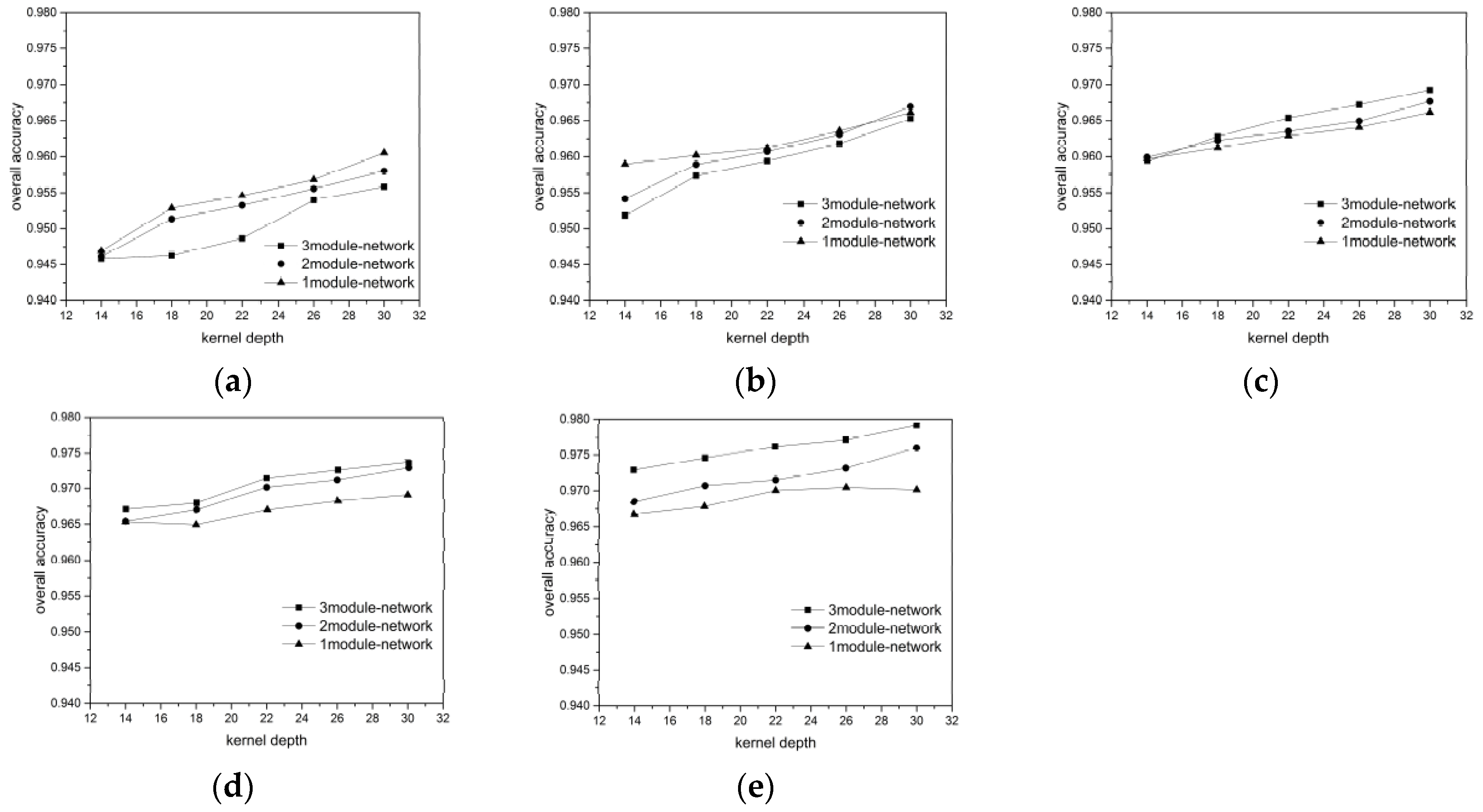
For each ground object category, we randomly chose 300, 400, 500, 600, and 700 labeled pixels as the training + validation data (ratio 7:3) to verify the influence of the training data volume on the network performance. The results are showing in Figure 11 and Figure 12, for the BJ02 and GF02 images, respectively.

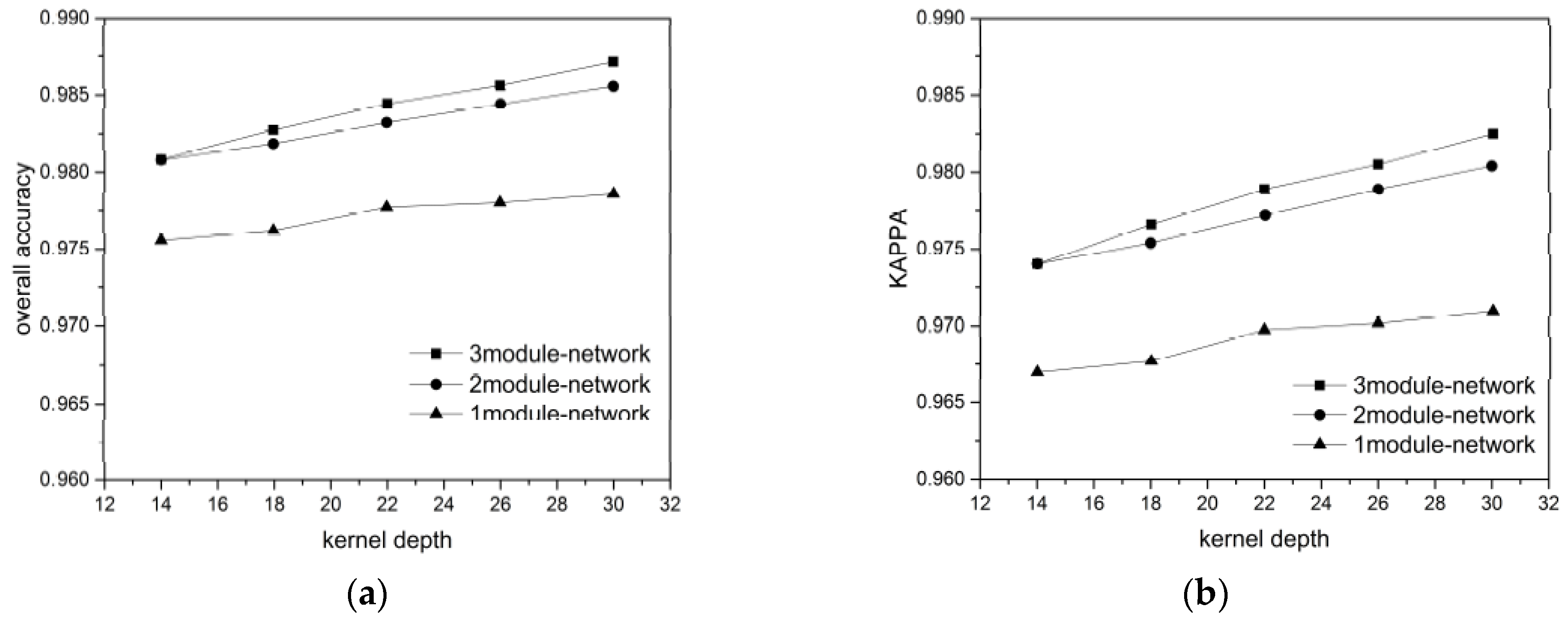
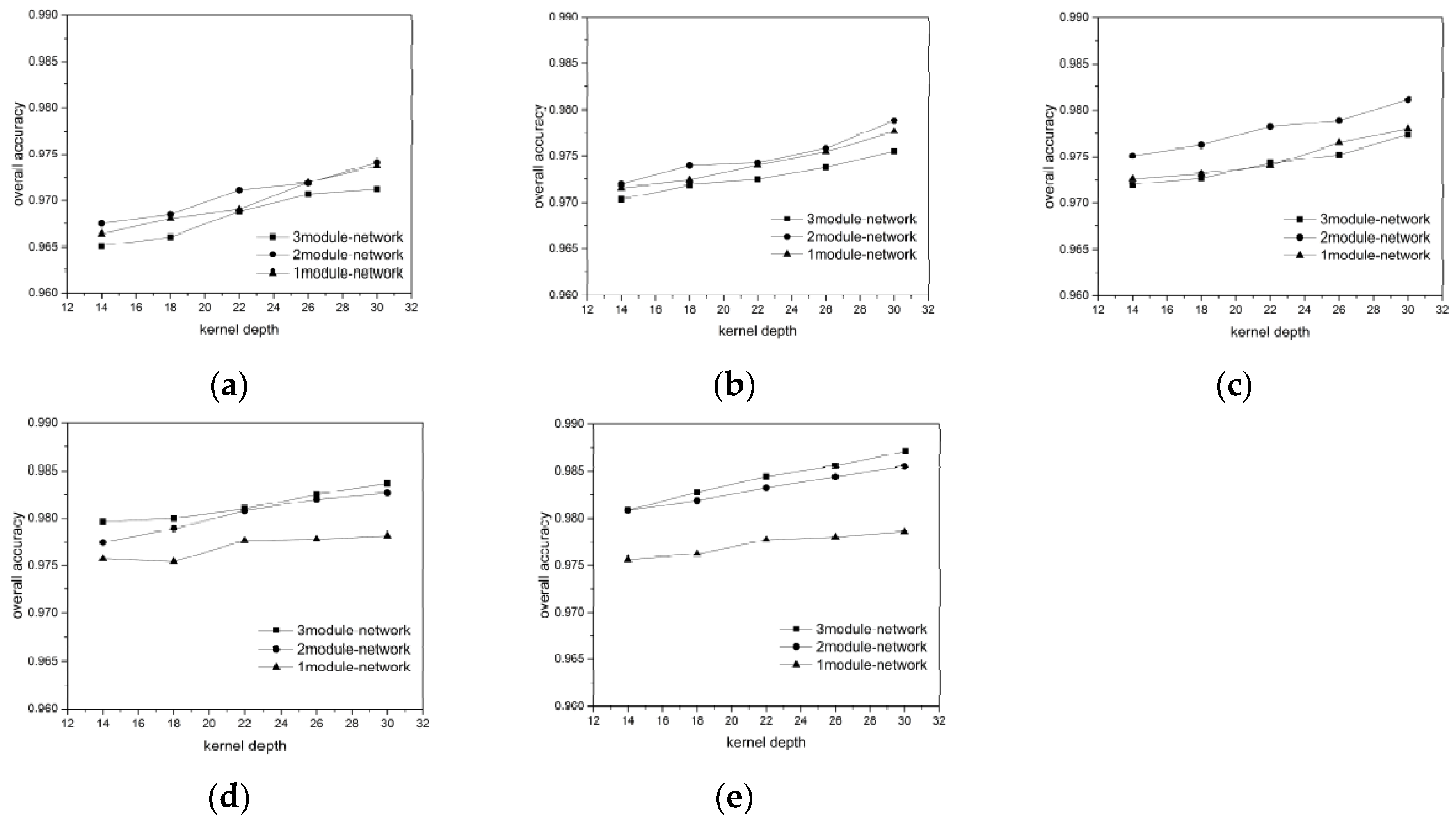
Considering the BJ02 and GF02 results, we found that the influence of the network depth on the network performance was affected by the training data volume. In our experiment, a longer network did not guarantee a superior classification result. For instance, when the 300 or 400 pixels/category training data were used for the BJ02 images, the network depth was inversely proportional to the classification accuracy. When the training data volume was small, the shallow networks achieved superior accuracy, with the shortest one achieving 96.1% OA and the longest one achieving only 95.6% OA. For GF02, when the training data volume was less than 500 pixels/category, the longest network exhibited the weakest performance. However, when the training data volume was small, the network length was not inversely proportional to the classification accuracy, unlike that for the BJ02 images. The 1-module networks exhibited only slightly poorer performance than the 2-module networks.

When the training data volume was 700 pixels/category, a deeper network corresponded to superior performance. This was because the number of parameters to be trained in the deep networks was greater than that in the shallow networks. When the labeled pixels were few, they became a burden for network training. Although we used a feedback attention or internal classifier mechanism to assist gradient propagation and to suppress the influence of overfitting, when the training data volume was small, the complexity of the deep networks induced more problems than encountered for the shallow networks. Nonetheless, when the training data volume was small, an increase in the number of convolutional kernels brought the deep network accuracy increasingly closer to that of the shallow networks. This indicates that the combined effect of the network depth and the number of convolutional kernels can assist the network in better extracting features for classification.

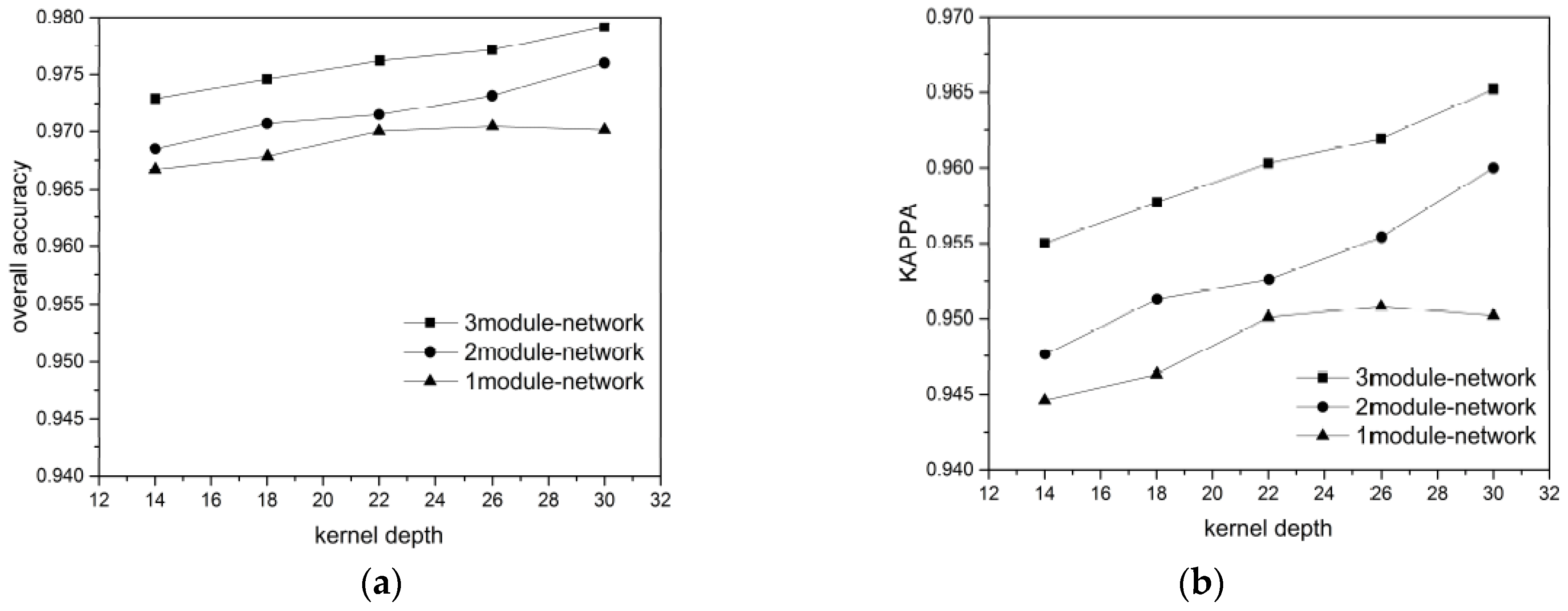
As the training data volume increased, the benefits of the deep networks emerged. The networks with larger numbers of modules could extract a greater number of hierarchical features using the added convolutional layers. The shallow layers extracted features with a greater focus on the ground-object details, such as their locations and boundaries, whereas the deeper layers extracted features that were more abstract, discriminative, and target-oriented. Therefore, the hierarchical features strengthened the expressive ability of the networks. Additionally, in our network design, one module comprised a mask branch and a trunk branch and different modules utilized different masks to focus on the features of the local spatial structures on different scales. Each module corresponded to a kind of attention. The mix of multiple attention types helped the networks handle more complex situations regarding ground objects. Therefore, for the BJ02 experiments, when the number of convolutional kernels was 30, the 3-module network could achieve an OA of approximately 98%, while the classification accuracy of the 1-module network was less than 97%. For the GF02 images, the networks stacked with 3 modules could achieve an OA exceeding 98.7% and a Kappa higher than 98.3%.

In addition, we found that the influences of the number of the convolutional kernels on the network performance differed with the training data. Taking the BJ02 results as an example, when the training data volume was small, the network classification accuracy increased rapidly and became more noticeable. However, as the training data volume increased, the classification accuracy increase became slower. When the network had just one module, the accuracy tended to remain stable even when the number of convolutional kernels increased. This may have been because the network required a larger number of feature detectors to identify the most discriminative features for ground object classification when there were fewer training samples. However, with an increase in the training data volume, the features most common and inherent to each category could be acquired even with fewer convolutional kernels by using a greater training data volume to train the network. Therefore, the benefits of the convolutional kernels were occluded and became less significant. Nonetheless, for the largest training data volume, the classification accuracy increased from 97.2% to 97.9% in the 3-module network when 14 and 30 kernels were used.

Furthermore, regarding the experimental results, when the training data volume decreased drastically, the network accuracy dropped gradually. This outcome demonstrated the network robustness and indicated that the networks could handle conditions involving a small volume of training data, which is very helpful for the remote sensing field.

4.2. Influence of Training Time

Comparison of the training times of the proposed method and the state-of-the-art methods mentioned in Section 3.2.3 revealed some limitations to our proposed method. Considerable feature reuse and feature fusion are involved in the network training; hence, a large amount of floating point arithmetic appears in the feed forward and backpropagation, and the kernels with different scales (especially 5 × 5 kernels) consume an extremely large amount of time for operations such as convolution. Therefore, with the Quadro K620 graphics card and a training data volume of 700 pixels/category, training a network with 3 modules and 30 kernels/convolution consumes 3.5 h. This training time is closer to that for the contextual deep CNN and DenseNet tested in Section 3.2.3. However, URDNN, DNN, and SCAE + SVM have considerably shorter training times, at less than 1 h. Training using SENet consumes approximately 2.5 h. Although the training time differs for each method, the classification times after training are all less than 1 s, which is acceptable. Therefore, decreasing the network complexity and improving its training efficiency will be our next research aim.

5. Conclusions

This paper has proposed a novel deep neural network fused with an attention mechanism to perform VHRRS image pixel-wise classification. The proposed network simulates the manner in which human beings comprehend images, emphasizing helpful information while suppressing unnecessary information, and thereby promoting sensibility toward informative features and providing convenience for superior information mining and image pixel-wise classification. The network is designed to have a “trunk branch” + “mask branch” structure. The feedback attention mechanism is implemented in the trunk branch, which applies feature reuse to return higher-level features to a lower level to re-assess the objective and re-weight the focus. In the mask branch, the neural network assigns a different priority to each pixel location by assigning different weights. Hence, attention is emphasized or suppressed and the neural network is aided in achieving end-to-end, pixel-to-pixel, pixel-wise classification. Furthermore, the proposed method adopts various masks with different scales to discern ground-object features on different scales. Through a 1 × 1 convolution mask, spectral information and the relationship among bands is found, while masks with larger scales help incorporate the surroundings and extract features from different local spatial structures. The internal classifiers enhance the effectiveness of the features extracted by hidden layers, thereby decreasing the feature redundancy.

We conducted detailed experiments on our proposed method using BJ02 and GF02 images. The proposed method achieved satisfactory accuracy for these images, with OA = 97.9%, Kappa = 96.5% and OA = 98.7%, Kappa = 98.3%, respectively. The experiments verified that the network structures have apparent influences on the network behavior. First, to a certain extent, an increase in the number of convolutional kernels can increase the network’s classification capability, because more feature maps help the network to cover additional kinds of features. However, in this work, we could still achieve satisfactory results by utilizing feature re-use, even though we adopted fewer kernels compared with other methods. Second, a deeper network is not always superior. In this work, when a small volume of labeled training data was utilized, the deeper network possessed more parameters to be trained. In such a case, training problems had a tendency to arise, which rendered the classification capability inversely proportional to the length of the network. However, when a greater volume of training data was used, networks with more modules usually yielded better results, exhibiting a relationship with the network length.

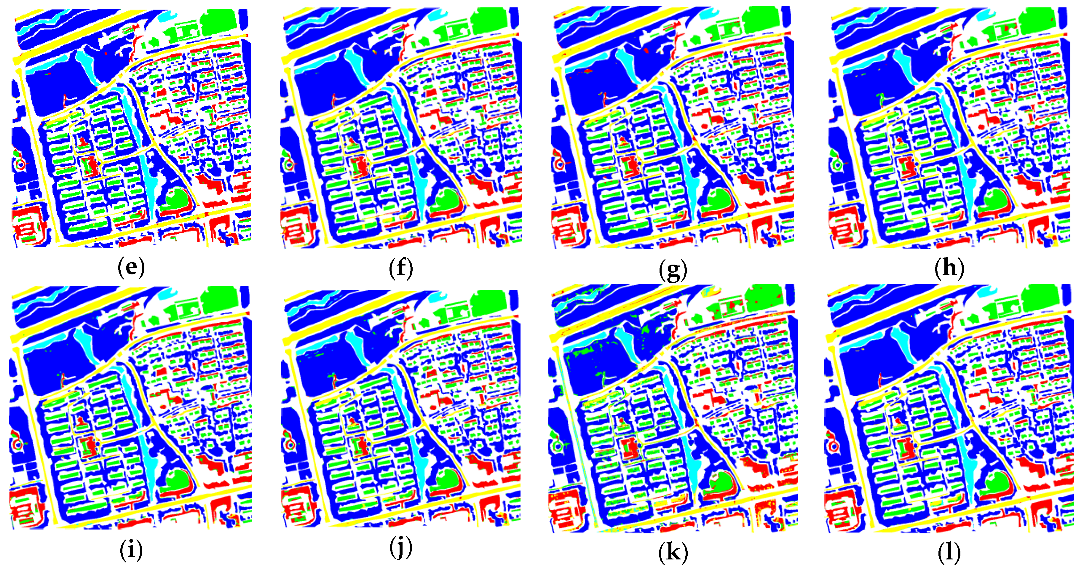
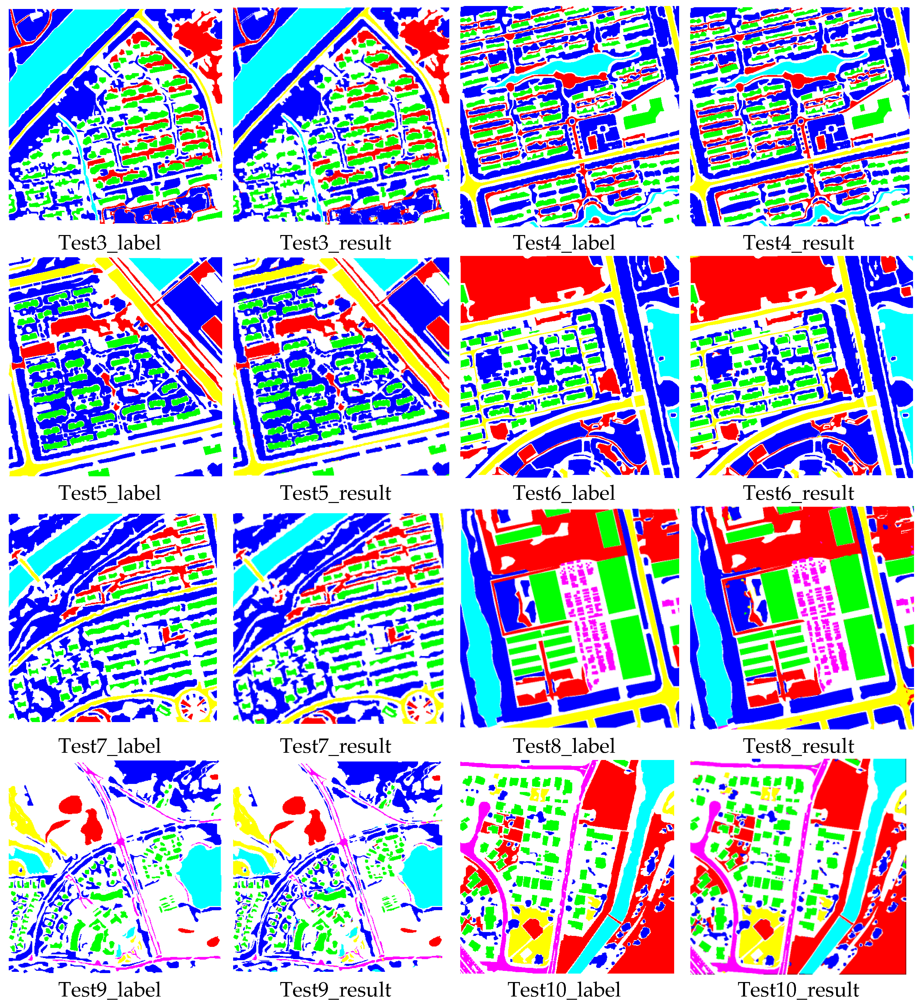
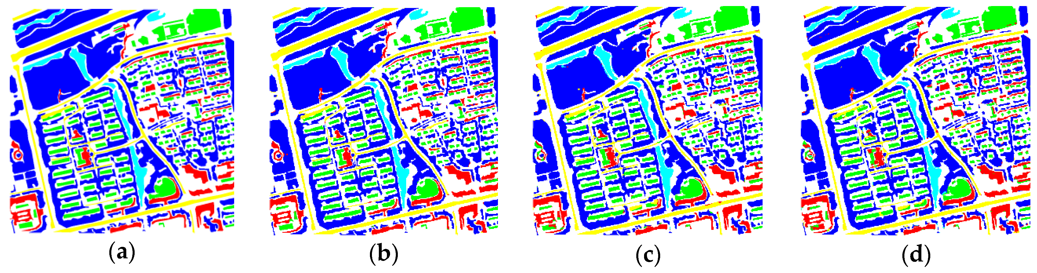
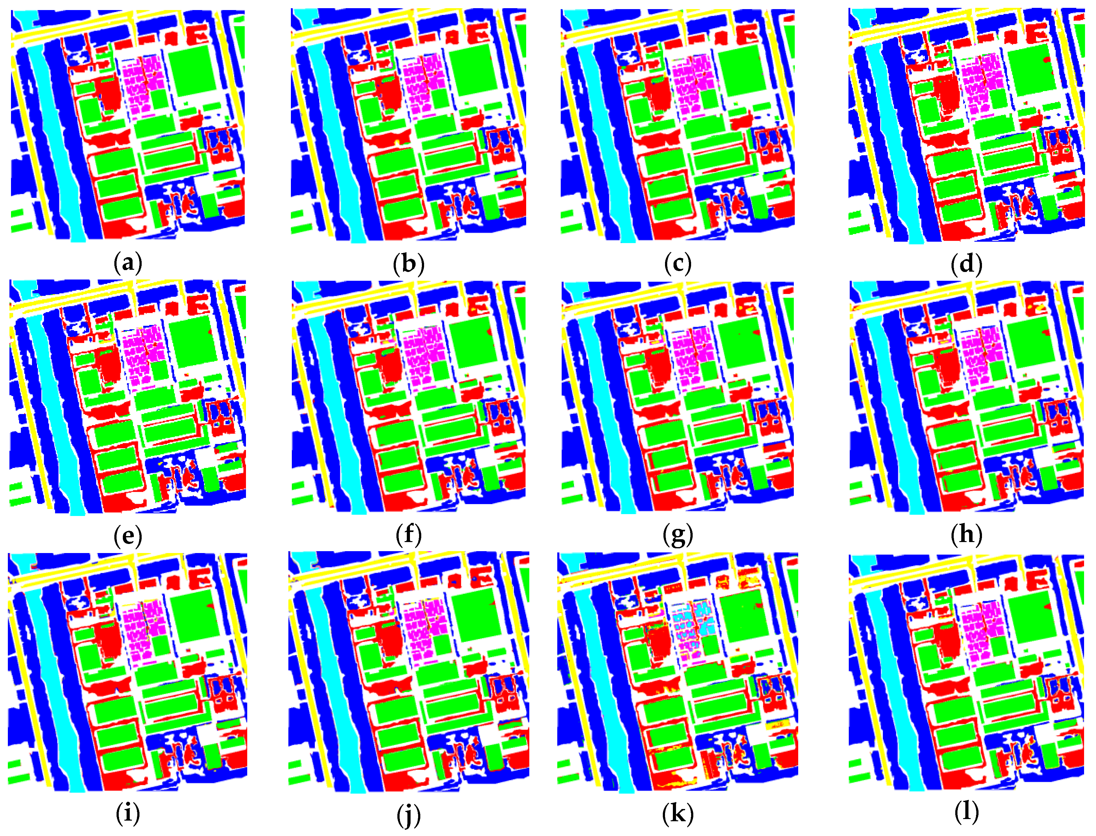
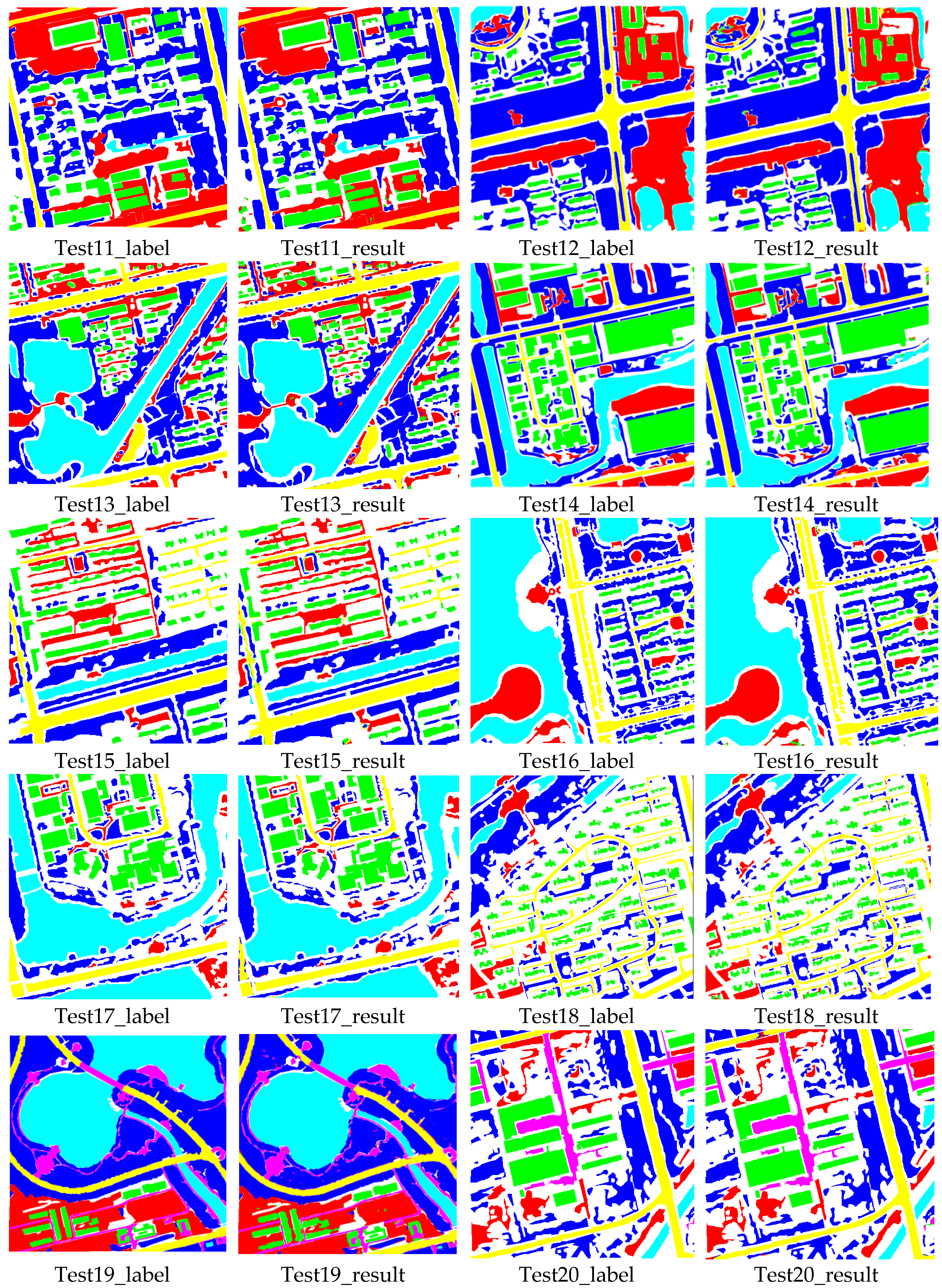
In the experiments, we also investigated the influence of the network components on the proposed method, and performed comparisons with some state-of-the-art methods, including methods with attention mechanisms and other popular methods. Furthermore, we applied the proposed method to additional images from the Quickbird, Geoeye, GF02, BJ02, etc., satellites, to verify the effectiveness and practicality of our method. In terms of accuracy and visual effects, the proposed method achieved competitive results. It not only yielded a higher accuracy, but also exhibited reduced confusion among some ground objects (such as buildings, bare land, and roads) compared with the other methods, and exhibited superior performance with regards to the edge preservation and interior integrity of ground objects.

To some degree, this work proved the effectiveness of this novel neural network for VHRRSI pixel-wise classification. In the near future, we plan to perform further research to adapt this method to fit more specific and complex applications such as object identification, so as to increase its feasibility for practical, real-world use.

References

1. Hwang, J.J.; Liu, T.L. Pixel-wise deep learning for contour detection. arXiv, 2015; arXiv:1504.01989. [Google Scholar]
2. Everingham, M.; Eslami, S.A.; Van Gool, L.; Williams, C.K.; Winn, J.; Zisserman, A. The pascal visual object classes challenge: A retrospective. Int. J. Comput. Vis. 2015, 111, 98–136. [Google Scholar] [CrossRef]
3. Huang, Z.; Cheng, G.; Wang, H.; Li, H.; Shi, L.; Pan, C. Building extraction from multi-source remote sensing images via deep deconvolution neural networks. In Proceedings of the 2016 IEEE International Geoscience and Remote Sensing Symposium (IGARSS), Beijing, China, 10–15 July 2016; pp. 1835–1838. [Google Scholar]
4. Wei, Y.; Wang, Z.; Xu, M. Road structure refined cnn for road extraction in aerial image. IEEE Geosci. Remote Sens. Lett. 2017, 14, 709–713. [Google Scholar] [CrossRef]
5. Hinton, G.E.; Salakhutdinov, R.R. Reducing the dimensionality of data with neural networks. Science 2006, 313, 504–507. [Google Scholar] [CrossRef] [PubMed]
6. He, K.; Zhang, X.; Ren, S.; Sun, J. Spatial pyramid pooling in deep convolutional networks for visual recognition. IEEE Trans. Pattern Anal. Mach. Intell. 2015, 37, 1904–1916. [Google Scholar] [CrossRef] [PubMed]
7. Paoletti, M.; Haut, J.; Plaza, J.; Plaza, A. A new deep convolutional neural network for fast hyperspectral image classification. ISPRS J. Photogramm. Remote Sens. 2017, 145, 120–147. [Google Scholar] [CrossRef]
8. Pacifici, F.; Del Frate, F.; Solimini, C.; Emery, W.J. An innovative neural-net method to detect temporal changes in high-resolution optical satellite imagery. IEEE Trans. Geosci. Remote Sens. 2007, 45, 2940–2952. [Google Scholar] [CrossRef]
9. Chen, Y.; Jiang, H.; Li, C.; Jia, X.; Ghamisi, P. Deep feature extraction and classification of hyperspectral images based on convolutional neural networks. IEEE Trans. Geosci. Remote Sens. 2016, 54, 6232–6251. [Google Scholar] [CrossRef]
10. Romero, A.; Gatta, C.; Camps-Valls, G. Unsupervised deep feature extraction for remote sensing image classification. IEEE Trans. Geosci. Remote Sens. 2016, 54, 1349–1362. [Google Scholar] [CrossRef]
11. Krizhevsky, A.; Sutskever, I.; Hinton, G.E. Imagenet classification with deep convolutional neural networks. In Proceedings of the Advances in Neural Information Processing Systems (NIPS), Harrahs and Harveys, NV, USA, 3–8 December 2012; pp. 1097–1105. [Google Scholar]
12. Simonyan, K.; Zisserman, A. Very deep convolutional networks for large-scale image recognition. arXiv, 2014; arXiv:1409.1556. [Google Scholar]
13. Szegedy, C.; Liu, W.; Jia, Y.; Sermanet, P.; Reed, S.; Anguelov, D.; Erhan, D.; Vanhoucke, V.; Rabinovich, A. Going deeper with convolutions. In Proceedings of the IEEE conference on Computer Vision and Pattern Recognition (CVPR), Boston, MA, USA, 8–10 June 2015; pp. 1–9. [Google Scholar]
14. He, K.; Zhang, X.; Ren, S.; Sun, J. Deep residual learning for image recognition. In Proceedings of the IEEE Conference on Computer Vision and Pattern Recognition (CVPR), Las Vegas, NV, USA, 26 June–1 July 2016; pp. 770–778. [Google Scholar]
15. Huang, G.; Sun, Y.; Liu, Z.; Sedra, D.; Weinberger, K.Q. Deep networks with stochastic depth. In Proceedings of the European Conference on Computer Vision (ECCV), Amsterdam, The Netherlands, 11–14 October 2016; Springer: Berlin, Germany, 2016; pp. 646–661. [Google Scholar]
16. Zhao, W.; Du, S. Spectral–spatial feature extraction for hyperspectral image classification: A dimension reduction and deep learning approach. IEEE Trans. Geosci. Remote Sens. 2016, 54, 4544–4554. [Google Scholar] [CrossRef]
17. Jabari, S.; Zhang, Y. Very high resolution satellite image classification using fuzzy rule-based systems. Algorithms 2013, 6, 762–781. [Google Scholar] [CrossRef]
18. Larochelle, H.; Hinton, G.E. Learning to combine foveal glimpses with a third-order boltzmann machine. In Proceedings of the Advances in Neural Information Processing Systems (NIPS), Vancouver, BC, Canada, 6–11 December 2010; pp. 1243–1251. [Google Scholar]
19. Mnih, V.; Heess, N.; Graves, A. Recurrent models of visual attention. In Proceedings of the Advances in Neural Information Processing Systems (NIPS), Montreal, QC, Canada, 8–13 December 2014; pp. 2204–2212. [Google Scholar]
20. Wang, F.; Jiang, M.; Qian, C.; Yang, S.; Li, C.; Zhang, H.; Wang, X.; Tang, X. Residual attention network for image classification. arXiv, 2017; arXiv:1704.06904. [Google Scholar]
21. Peng, Y.; He, X.; Zhao, J. Object-part attention model for fine-grained image classification. IEEE Trans. Image Process. 2018, 27, 1487–1500. [Google Scholar] [CrossRef] [PubMed]
22. Zhu, Y.; Zhao, C.; Guo, H.; Wang, J.; Zhao, X.; Lu, H. Attention couplenet: Fully convolutional attention coupling network for object detection. IEEE Trans. Image Process. 2018, 28, 113–126. [Google Scholar] [CrossRef] [PubMed]
23. Cao, C.; Liu, X.; Yang, Y.; Yu, Y.; Wang, J.; Wang, Z.; Huang, Y.; Wang, L.; Huang, C.; Xu, W. Look and think twice: Capturing top-down visual attention with feedback convolutional neural networks. In Proceedings of the IEEE International Conference on Computer Vision (ICCV), Santiago, Chile, 13–16 December 2015; pp. 2956–2964. [Google Scholar]
24. Nam, H.; Ha, J.-W.; Kim, J. Dual attention networks for multimodal reasoning and matching. arXiv, 2016; arXiv:1611.00471. [Google Scholar]
25. Zhang, F.; Du, B.; Zhang, L. Saliency-guided unsupervised feature learning for scene classification. IEEE Trans. Geosci. Remote Sens. 2015, 53, 2175–2184. [Google Scholar] [CrossRef]
26. Hu, J.; Xia, G.-S.; Hu, F.; Sun, H.; Zhang, L. A comparative study of sampling analysis in scene classification of high-resolution remote sensing imagery. In Proceedings of the 2015 IEEE International Geoscience and Remote Sensing Symposium (IGARSS), Milan, Italy, 26–31 July 2015; pp. 2389–2392. [Google Scholar]
27. Chen, J.; Wang, C.; Ma, Z.; Chen, J.; He, D.; Ackland, S. Remote sensing scene classification based on convolutional neural networks pre-trained using attention-guided sparse filters. Remote Sens. 2018, 10, 290. [Google Scholar] [CrossRef]
28. Hu, J.; Shen, L.; Sun, G. Squeeze-and-excitation networks. arXiv, 2017; arXiv:1709.01507. [Google Scholar]
29. Yang, Y.; Zhong, Z.; Shen, T.; Lin, Z. Convolutional neural networks with alternately updated clique. In Proceedings of the IEEE Conference on Computer Vision and Pattern Recognition (CVPR), Salt Lake City, UT, USA, 19–21 June 2018; pp. 2413–2422. [Google Scholar]
30. Kim, J.-H.; Lee, S.-W.; Kwak, D.; Heo, M.-O.; Kim, J.; Ha, J.-W.; Zhang, B.-T. Multimodal residual learning for visual qa. In Proceedings of the Advances in Neural Information Processing Systems (NIPS), Barcelona, Spain, 5–10 December 2016; pp. 361–369. [Google Scholar]
31. Chen, L.-C.; Yang, Y.; Wang, J.; Xu, W.; Yuille, A.L. Attention to scale: Scale-aware semantic image segmentation. In Proceedings of the IEEE Conference on Computer Vision and Pattern Recognition (CVPR), Las Vegas, NV, USA, 27–30 June 2016; pp. 3640–3649. [Google Scholar]
32. Kong, S.; Fowlkes, C. Pixel-wise attentional gating for parsimonious pixel labeling. arXiv, 2018; arXiv:1805.01556. [Google Scholar]
33. Fu, J.; Liu, J.; Tian, H.; Fang, Z.; Lu, H. Dual attention network for scene segmentation. arXiv, 2018; arXiv:1809.02983. [Google Scholar]
34. Hopfinger, J.B.; Buonocore, M.H.; Mangun, G.R. The neural mechanisms of top-down attentional control. Nat. Neurosci. 2000, 3, 284. [Google Scholar] [CrossRef] [PubMed]
35. Huang, G.; Liu, Z.; Van Der Maaten, L.; Weinberger, K.Q. Densely connected convolutional networks. In Proceedings of the IEEE Conference on Computer Vision and Pattern Recognition (CVPR), Honolulu, HI, USA, 21–26 July 2017; p. 3. [Google Scholar]
36. Li, E.; Xia, J.; Du, P.; Lin, C.; Samat, A. Integrating multilayer features of convolutional neural networks for remote sensing scene classification. IEEE Trans. Geosci. Remote Sens. 2017, 55, 5653–5665. [Google Scholar] [CrossRef]
37. Yu, Y.; Gong, Z.; Wang, C.; Zhong, P. An unsupervised convolutional feature fusion network for deep representation of remote sensing images. IEEE Geosci. Remote Sens. Lett. 2018, 15, 23–27. [Google Scholar] [CrossRef]
38. Song, W.; Li, S.; Fang, L.; Lu, T. Hyperspectral image classification with deep feature fusion network. IEEE Trans. Geosci. Remote Sens. 2018, 56, 3173–3184. [Google Scholar] [CrossRef]
39. Lee, H.; Kwon, H. Going deeper with contextual cnn for hyperspectral image classification. IEEE Trans. Image Process. 2017, 26, 4843–4855. [Google Scholar] [CrossRef] [PubMed]
40. Tao, Y.; Xu, M.; Lu, Z.; Zhong, Y. Densenet-based depth-width double reinforced deep learning neural network for high-resolution remote sensing image pixel-wise classification. Remote Sens. 2018, 10, 779. [Google Scholar] [CrossRef]
41. Bansal, A.; Chen, X.; Russell, B.; Gupta, A.; Ramanan, D. Pixelnet: Representation of the pixels, by the pixels, and for the pixels. arXiv, 2017; arXiv:1702.06506. [Google Scholar]
42. Tao, Y.; Xu, M.; Zhang, F.; Du, B.; Zhang, L. Unsupervised-restricted deconvolutional neural network for very high resolution remote-sensing image classification. IEEE Trans. Geosci. Remote Sens. 2017, 55, 6805–6823. [Google Scholar] [CrossRef]
43. Glorot, X.; Bengio, Y. Understanding the difficulty of training deep feedforward neural networks. In Proceedings of the Thirteenth International Conference on Artificial Intelligence and Statistics, Sardinia, Italy, 13–15 May 2010; pp. 249–256. [Google Scholar]
44. Yu, F.; Koltun, V. Multi-scale context aggregation by dilated convolutions. arXiv, 2015; arXiv:1511.07122. [Google Scholar]
45. Pinheiro, P.O.; Collobert, R. From image-level to pixel-level labeling with convolutional networks. In Proceedings of the IEEE Conference on Computer Vision and Pattern Recognition (CVPR), Boston, MA, USA, 8–10 June 2015; pp. 1713–1721. [Google Scholar]
46. Bengio, Y.; Lamblin, P.; Popovici, D.; Larochelle, H. Greedy layer-wise training of deep networks. In Proceedings of the Advances in Neural Information Processing Systems (NIPS), Vancouver, BC, Canada, 3–6 December 2007; pp. 153–160. [Google Scholar]
47. Lee, C.Y.; Xie, S.; Gallagher, P.; Zhang, Z.; Tu, Z. Deeply-supervised nets. In Proceedings of the Artificial Intelligence and Statistics, San Diego, CA, USA, 9–12 May 2015; pp. 562–570. [Google Scholar]
48. Shi, Q.; Du, B.; Zhang, L. Domain adaptation for remote sensing image classification: A low-rank reconstruction and instance weighting label propagation inspired algorithm. IEEE Trans. Geosci. Remote Sens. 2015, 53, 5677–5689. [Google Scholar]
49. Coates, A.; Ng, A.; Lee, H. In An analysis of single-layer networks in unsupervised feature learning. In Proceedings of the Fourteenth International Conference on Artificial Intelligence and Statistics, Lauderdale, FL, USA, 11–13 April 2011; pp. 215–223. [Google Scholar]
50. Volpi, M.; Tuia, D. Dense semantic labeling of subdecimeter resolution images with convolutional neural networks. IEEE Trans. Geosci. Remote Sens. 2017, 55, 881–893. [Google Scholar] [CrossRef]
Figure 1. The flowchart of the proposed attention-mechanism-containing neural network.
Remotesensing 10 01602 g001
Figure 2. The flowchart of feedforward and feedback stages. The numbers in the flowchart represent the calculation sequence in the feedback stages. The red lines indicate that the higher-level features are returned to update the previous-level feature extraction so that it becomes more objective-oriented.
Remotesensing 10 01602 g002
Figure 3. The dilated convolution operation.
Remotesensing 10 01602 g003
Figure 4. The fusion of the two attention mechanisms.
Remotesensing 10 01602 g004
Figure 5. The twenty images used in the experiment: (ad) From the BJ02 satellite; (er) from the GF02 satellite; and (s,t) from the Geoeye and Quickbird satellites, respectively.
Remotesensing 10 01602 g005
Figure 6. (a,b) The OA and Kappa coefficients, respectively, acquired from the BJ02 images with 700 pixels/category of training data based on different network structures.
Remotesensing 10 01602 g006
Figure 7. (a,b) The OA and Kappa coefficients, respectively, acquired from the GF02 images with 700 pixels/category of training data based on different network structures.
Remotesensing 10 01602 g007
Figure 8. The BJ02 classification results given by (a) manually labeled reference data; (b) the proposed method; (c) the internal-classifier-removed network; (d) the feedback-attention-removed network; (e) the mask-attention-removed network; (f) CNN; (g) contextual deep CNN; (h) DenseNet; (i) the unsupervised-restricted DNN(URDNN); (j) the deconvolutional neural network (DNN); (k) SCAE + SVM; and (l) Squeeze-and-Excitation Networks (SENet).
Remotesensing 10 01602 g008aRemotesensing 10 01602 g008b
Figure 9. The GF02 classification results given by (a) manually labeled reference data; (b) the proposed method; (c) the internal-classifier-removed network; (d) the feedback-attention-removed network, (e) the mask-attention-removed network; (f) CNN; (g) contextual deep CNN; (h) DenseNet; (i) URDNN; (j) DNN; (k) SCAE + SVM; and (l) SENet.
Remotesensing 10 01602 g009
Figure 10. The classification results of the proposed method for the remaining eight experiments.
Remotesensing 10 01602 g010aRemotesensing 10 01602 g010b
Figure 11. (ae) The overall accuracy acquired for the BJ02 images with 300, 400, 500, 600, and 700 pixels/category of training data, respectively, based on different network structures.
Remotesensing 10 01602 g011
Figure 12. (ae) The overall accuracy acquired for the GF02 images with 300, 400, 500, 600, and 700 pixels/category of training data, respectively, based on the different network structures.
Remotesensing 10 01602 g012