Hyperspectral Unmixing with Bandwise Generalized Bilinear Model


1
Department of Biomedical Engineering, Hefei University of Technology, Hefei 230009, China
2
Department of Electronic Science and Technology, University of Science and Technology of China, Hefei 230027, China
*
Author to whom correspondence should be addressed.
Remote Sens. 2018, 10(10), 1600; https://doi.org/10.3390/rs10101600
Submission received: 5 September 2018
/
Revised: 30 September 2018
/
Accepted: 6 October 2018
/
Published: 9 October 2018
(This article belongs to the Special Issue Robust Multispectral/Hyperspectral Image Analysis and Classification)
Abstract
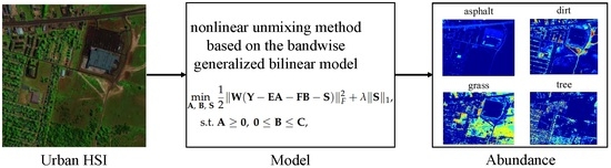
:Generalized bilinear model (GBM) has received extensive attention in the field of hyperspectral nonlinear unmixing. Traditional GBM unmixing methods are usually assumed to be degraded only by additive white Gaussian noise (AWGN), and the intensity of AWGN in each band of hyperspectral image (HSI) is assumed to be the same. However, the real HSIs are usually degraded by mixture of various kinds of noise, which include Gaussian noise, impulse noise, dead pixels or lines, stripes, and so on. Besides, the intensity of AWGN is usually different for each band of HSI. To address the above mentioned issues, we propose a novel nonlinear unmixing method based on the bandwise generalized bilinear model (NU-BGBM), which can be adapted to the presence of complex mixed noise in real HSI. Besides, the alternative direction method of multipliers (ADMM) is adopted to solve the proposed NU-BGBM. Finally, extensive experiments are conducted to demonstrate the effectiveness of the proposed NU-BGBM compared with some other state-of-the-art unmixing methods.
1. Introduction
Hyperspectral images (HSIs) are usually acquired in hundreds of narrow contiguous spectral bands by a specific kind of imaging sensor, e.g., the Airborne Visible/Infrared Imaging Spectrometer, Hyperspectral Digital Imagery Collection Experiment and Compact Airborne Spectrographic Imager [1,2,3]. Due to the high spectral resolution, it is inevitable to bring about the problem of “mixed pixels”, and different materials usually occupy a single hyperspectral pixel [4,5,6]. The existence of mixed pixels have a large impact on many applications, such as object detection [7], subpixel mapping [8], classification [9,10,11,12], and matching [13,14,15]. Thus, hyperspectral unmixing has been exploited to decompose mixed pixels into a group of pure materials (called endmembers) and their corresponding proportions (called abundances) [16,17].
The linear mixing model (LMM) is a simple and widely used unmixing model. Each pixel can be formulated as a linear combination of endmembers with additional noise. The idea is that each incoming light ray interacts with only one material before reaching the sensor [18,19]. However, the LMM is invalid when there are intimate mixtures, terrain relief, or volumetric scattering [20]. Nonlinear mixing models (NLMMs) provide an alternative to take the above mentioned problem into account, which can be generally divided into two categories [20,21]. The first category includes some flexible models based on signal processing, such as post-nonlinear model [22], neural network model [23] and kernel model [24]. The second category includes some physical based models, such as intimate mixture model [25], bilinear mixture model (BMM) [26,27,28,29,30,31,32,33] and multilinear mixing model [34,35,36]. Among them, the BMM only takes the second-order scattering into consideration, while the higher-order interactions of light are ignored [18]. The reason is that the interactions of orders larger than two, not only have minor contribution for improving the unmixing accuracy than that of second-order scattering, but also bring in tremendous computational costs [21]. Several representative models known as the family of BMM have been proposed. The Nascimento model (NM) [26] is an extended LMM with additional virtual endmembers, the Fan’s model (FM) is the truncated Taylor expansion of nonlinear mixing function [27], and the GBM [28] can be seen as the generalization of LMM and FM, which can efficiently deal with the assumptions in BMM. Different methods have been proposed for GBM unmixing of HSI, Halimi et al. developed a Bayesian algorithm to estimate the abundance and noise variance of the GBM [28]. Besides, they also proposed a pixel-wise unmixing method based on the gradient descent algorithm (GDA) [29]. Moreover, Yokoya et al. proposed the semi-nonnegative matrix factorization (semi-NMF) as a new optimization method for GBM based HSI unmixing [30]. Furthermore, Li et al. developed the bound projected optimal gradient method (BPOGM) for GBM unmixng, and it can achieve the optimal convergence rate of , where k denotes the number of iteration in BPOGM [31].
Most unmixing methods based on the GBM are implicitly developed for Gaussian noise, and the underlying assumption is that the intensities of Gaussian noise remain the same for different bands of HSI. However, there remain two challenges for many real applications of GBM based hyperspectral unmixing. One is that each band of HSI is degraded by different intensities of AWGN, and the other is the widely existed mixed noise in real HSI, including Gaussian noise, impulse noise, dead pixels or lines, stripes and so on [37,38,39,40]. Aggarwal et al. proposed a hyperspectral unmixing method in the presence of mixed noise using joint-sparsity and total variation, which can take several kinds of noise into consideration [41]. However, it still ignored the nonlinear mixing effect and the different intensities of AWGN in different bands of HSI. In this paper, to overcome the above mentioned problems, we propose a novel nonlinear unmixing method based on the bandwise generalized bilinear model (NU-BGBM). First, a bandwise generalized bilinear model (BGBM) is proposed to take the complex mixed noise in real HSI into consideration, i.e., each band of HSI is contaminated by different types of noise, and the AWGN intensities of across different bands are assumed to be different. Second, a novel method based on the BGBM is proposed under the maximum a posteriori framework. The diagonal of weight matrix is the reciprocal of the variance of AWGN in each band, which can take the different intensities of AWGN in different bands into consideration. The impulse noise, dead pixels or lines, and stripes usually contaminate a small part of the whole HSI, which usually have the underlying sparse property.
The main contributions of this work lie in that we propose a BGBM to be adapted for complex mixed noise in real HSI. Besides, we propose a novel NU-BGBM under the maximum a posteriori framework, which can take different types of noise into consideration. Moreover, we use the alternative direction method of multipliers (ADMM) [42] for solving the proposed NU-BGBM. Finally, we conduct extensive experiments using both simulated and real HSIs to demonstrate the effectiveness and advantages of the proposed NU-BGBM.
The remainder of this paper is organized as follows. In Section 2, we introduce the related GBM and the formulation of the proposed NU-BGBM, and develop the ADMM for solving the proposed NU-BGBM. In Section 3, we demonstrate the efficiency and advantages of the proposed NU-BGBM on both simulated datasets and real HSIs. Finally, we conclude this paper in Section 4.
2. Bandwise Generalized Bilinear Model and Algorithm
In this section, we will introduce the related GBM at first. Then, we will introduce the proposed nonlinear unmixing model BGBM, and formulate the proposed unmixing method NU-BGBM in detail. Finally, we will solve the proposed NU-BGBM under the ADMM scheme.
2.1. The Related GBM
The LMM assumes that each pixel containing D bands in HSI is a linear combination of M endmembers as follows:
where the linear representation vector denotes the abundance, and represents the additive noise in HSI. The abundances usually have to meet two constraints, i.e., abundance non-negativity constraint (ANC) and abundance sum to one constraint (ASC) as follows:
However, the real HSI usually has strong signature variability [43], and the abundances may not meet the ASC constraint in practice, so we do not explicitly impose the ASC constraint for unmixing of HSI in this paper.
As noted in the introduction, the LMM may not always hold true in many situations. To take the multi-scattering radiation among different endmembers into consideration, BMM takes the second-order scattering into consideration, which is equivalent to add an additional second-order interaction term to LMM as follows:
where denotes the amount of nonlinearities between the ith and jth endmembers, and ⊙ is the Hadamard product operation. By imposing various constraints on the nonlinear coefficient in BMM, many different kinds of BMMs have been proposed, which include NM [26], FM [27], GBM [28,29,30,31], MGBM [44] and so on. Among them, the GBM can be seen as the generalization of LMM and FM, it sets the nonlinear coefficient , and the constraints imposed on the GBM can be written as follows:
Mathematically, the GBM for HSI having P pixels can be expressed as follows:
where denotes the reshaped HSI matrix, is the abundance matrix, denotes the bilinear endmember matrix, is the bilinear abundance matrix, and denotes the noise matrix. Therefore, the constraints imposed on the GBM having P pixels can be written as follows:
where .
2.2. Formulation of the Proposed BGBM and the Corresponding Unmixing Method NU-BGBM
The traditional GBM unmixing methods are implicitly developed in the presence of additive white Gaussian noise (AWGN), and the intensity of AWGN is assumed to be the same for each band of HSI. However, the HSIs in real world are usually degraded by mixed noise, i.e., the HSI is usually polluted by not only the Gaussian noise, but also other types of noise, such as impulse noise, dead pixels or lines, and stripes [37,38,39,40]. Besides, the intensity of AWGN is usually different for different band of HSI. The noise in real HSI can be generally classified into two classes, i.e., dense noise and sparse noise. The dense noise means that most of the HSI is contaminated, which mainly includes Gaussian noise. While the sparse noise means that only a small part of the HSI is contaminated, which mainly includes impulse noise, dead pixels or lines, and stripes. Therefore, the proposed bandwise unmixing model BGBM can be written as follows:
where , , , and represent the ith band of , , , and , respectively. and denote the sparse noise and dense Gaussian noise of HSI, respectively. We assume that the AWGN of each band is independent with different intensities of Gaussian noise, , and represent the variance of Gaussian noise in ith band, so we can obtain . Since the AWGN of each band is independent, so we can get
where c denotes a constant, represents the Frobenius norm. is the diagonal matrix, and , the diagonal matrix can be seen as a weighting matrix, the larger the variance of Gaussian noise is, the smaller the weight of the band is, so the weighting matrix can take different intensities of AWGN in different bands of HSI into consideration. Then, the abundances, bilinear abundance and the sparse noise of BGBM can be estimated under the maximum a posteriori framework as follows:
where represents the prior distribution of , which can be regarded as prior knowledge or constraints enforced on the abundances, bilinear abundance and the sparse noise of BGBM.
For the abundances and bilinear abundance of BGBM, they should also satisfy the constraints in Equation (6). For the sparse noise of BGBM, it has the underlying property of sparsity. The sparsity of sparse noise in BGBM can be ideally represented by the norm. However, norm based optimization is usually NP-hard to solve, so we replace the norm with norm. Thus, the proposed nonlinear unmixing method based on the BGBM can be formulated as follows:
where is the regularization parameter to strike a balance between the reconstruction error and the sparse regularization term, and .
2.3. Solving the Proposed NU-BGBM with ADMM
The ADMM has been widely used for solving the constrained optimization problems, and it has obtained desirable performance in many different kinds of applications as well as hyperspectral unmixing [20,44,45]. To get more details of ADMM, please refer to [42]. Here, we provide details of adopting ADMM to solve the proposed NU-BGBM.
The model in Equation (10) can be reformulated as follows:
where denotes the indicator function for the nonnegative orthant , is the -th element of , and is zero when belongs to the nonnegative orthant, and otherwise. is the indicator function for the interval , and is zero when belongs to the interval , and otherwise. , and denote three auxiliary variables.
Equation (11) can be reformulated using the compact form as follows:
where , , , , , .
The augmented Lagrangian function can be written as follows:
where denotes the penalty parameter, is the Lagrange multipliers. Therefore, we can sequentially optimize with respect to , and .
To update , we solve
To update , we solve
To update , we solve
where represents the element-wise soft shrinkage operator [46], and denotes the threshold.
To update , we solve
To update , we solve
To update , we solve
The primal and dual residuals and can be written as follows:
According to [42], the stopping criterion can be written as follows:
According to [42], has a large impact on the convergence speed, we update to keep the ratio between the primal norms and dual residual norms within a given positive interval, and they both converge to zero. When adopting the ADMM to solve the proposed NU-BGBM, we need to know the weighting matrix before hand, i.e., estimating the stand deviation of AWGN for different bands of HSI. In this paper, the hyperspectral signal identification by minimum error (HySime) [47] is used to estimate the noise of HSI. The HySime assumes that there are usually high correlation among the neighboring bands of HSI, which can be solved by the multiple regression theory. Therefore, the detailed procedure for solving the proposed NU-BGBM is summarized in Algorithm 1.
| Algorithm 1: Solving the proposed NU-BGBM with ADMM. |
 |
3. Experiments
In this section, we conduct experiments on both synthetic datasets and real HSIs to demonstrate efficiency and advantages of the proposed NU-BGBM. We compare the unmixing performance of the proposed NU-BGBM with the other four methods, i.e., the fully constrained least squares (FCLS) algorithm [48], GDA [29], semi-NMF [30] and BPOGM [31]. The FCLS is based on the LMM, the other three compared methods are all based on the GBM.
For the four compared methods, we adopt the recommended default parameters in the original references. For the proposed NU-BGBM, there are mainly four parameters, i.e., the regularization parameter , the Lagrange multiplier regularization parameter , the error tolerance and the maximum number of iteration N. We have found that the regularization parameter has much larger impact on the unmixing performance than the other three parameters. Thus, throughout the experiments, we fix , and , and tune {, , , , , 1, , , , , }. Besides, since the GDA would diverge using random initialization [31], so all the GBM based unmixing methods are initialized by FCLS [48] for fair of comparison.
3.1. Experimental Results with Synthetic Data
In this subsection, we will conduct experiments on synthetic data to demonstrate efficiency and advantages of the proposed NU-BGBM in the presence of mixed noise. The bilinear mixing effect often appears between soil and vegetation [30,31], and we select six spectra from the U. S. Geological Survey (USGS) spectral library available at: http://speclab.cr.usgs.gov/spectral-lib.html, i.e., one type of water (Water+Montmor), two types of soil (Stonewall and Rangeland), and three types of vegetation (spurge, oak and pine). We downsample the original selected six spectra to P = 200 bands, and the spectra of them are shown in Figure 1, which are chosen as the six endmembers in the simulated experiment. After obtaining the endmember matrix , the bilinear endmember matrix can be naturally obtained according to BGBM. Then, we generate the abundance matrix of six selected endmembers according to [49], and the code is available at: https://bitbucket.org/aicip/mvcnmf. The synthetic HSI has 64 × 64 pixels having no pure pixels, the HSI is divided into 8 × 8 blocks and all pixels in each block are filled up by one of endmembers randomly selected from the selected six endmembers. The spatial low-pass filter of size 9 × 9 has been applied to the HSI to create linear mixture, and all pixels with abundances greater than 80% have been replaced by a mixture of all endmembers with equally distributed abundances, which aims at removing the probable pure pixels in the resulted HSI, and the generated abundances of the six endmembers are shown in the first row in Figure 2. The nonlinearity coefficients are uniformly drawn in the interval [0, 1], and the bilinear abundance matrix can be also obtained according to BGBM. Then, three kinds of noise will be added to the HSI to simulate the mixed noise and different intensities of AWGN in each band of HSI in practice:
- Gaussian noise: all bands of the HSI are contaminated by zero mean i.i.d. Gaussian noise, and the signal-to-noise ratio (SNR) of each band is a random number ranging from 10 dB to 50 dB.
- Impulse noise: only 11 bands (60–70) are contaminated by 30% impulse noise.
- Dead lines: only 11 bands (120–130) are contaminated by dead lines.
To simulate the mixed noise in real HSI as much as possible, we conduct experiments in the presence of one type of noise, two types of noise and three types of noise, which can be seen in Table 1. After adding noise to the synthetic HSI, we adopt the compared methods and the proposed NU-BGBM to unmix the synthetic HSIs using the given true endmembers. To evaluate the unmixing performances of different methods, we adopt the root mean square error (RMSE) [30,31] as the quantitative evaluation criterion. Generally speaking, smaller RMSE indicates better HSI unmixing performance.
Table 1 gives the RMSEs of the compared methods and the proposed NU-BGBM in the presence of different types of noise. From Table 1, we can clearly see that when the synthetic HSI is only contaminated by Gaussian noise with different intensities for each band of HSI, the proposed NU-BGBM can obtain better unmixing performance than the other compared methods. This is due to that only our NU-BGBM can take the different intensities of AWGN in different bands into account under the maximum a posteriori framework. When the HSI is only degraded by impulse noise or dead lines, the proposed NU-BGBM can obtain much better unmixing performance than the other four compared methods, the underlying reason is that only our NU-BGBM can take the underlying sparsity of sparse noise into account, and the four compared methods all adopt the vector norm or the matrix Frobenius norm, but the vector norm or the matrix Frobenius norm is usually sensitive to non-Gaussian noise, and it would seriously degrade the unmixing performance in the presence of non-Gaussian noise. In the presence of two types of noise and three types of noise, the proposed NU-BGBM can also obtain better unmixing performances than the other compared methods, which demonstrate that our proposed method based on BGBM can handle the mixed noise and different intensities of AWGN in different bands efficiently, and hence our method is more robust and applicable than the other compared methods in the presence of complex mixed noise. Besides, the FCLS generally has worse unmixing performance than the other methods, this is due to that the FCLS is based on LMM, and the other methods are based on GBM or BGBM, which demonstrates the importance of taking nonlinear mixing effect into account to improve the accuracy of HSI unmixing. Furthermore, Figure 2 shows the abundance maps estimated by the compared methods and the proposed method in the presence of three types of noise, i.e., the synthetic HSI is contaminated by Gaussian noise, impulse noise and dead lines simultaneously. It can be clearly observed from Figure 2 that the abundances of six endmembers estimated by the proposed NU-BGBM can approximate obviously better to the ground truth than the other compared methods, which also demonstrate that our proposed NU-BGBM is more robust for the mixed noise and different intensities of AWGN in different bands than the other compared methods.
3.2. Experimental Results with Real Data
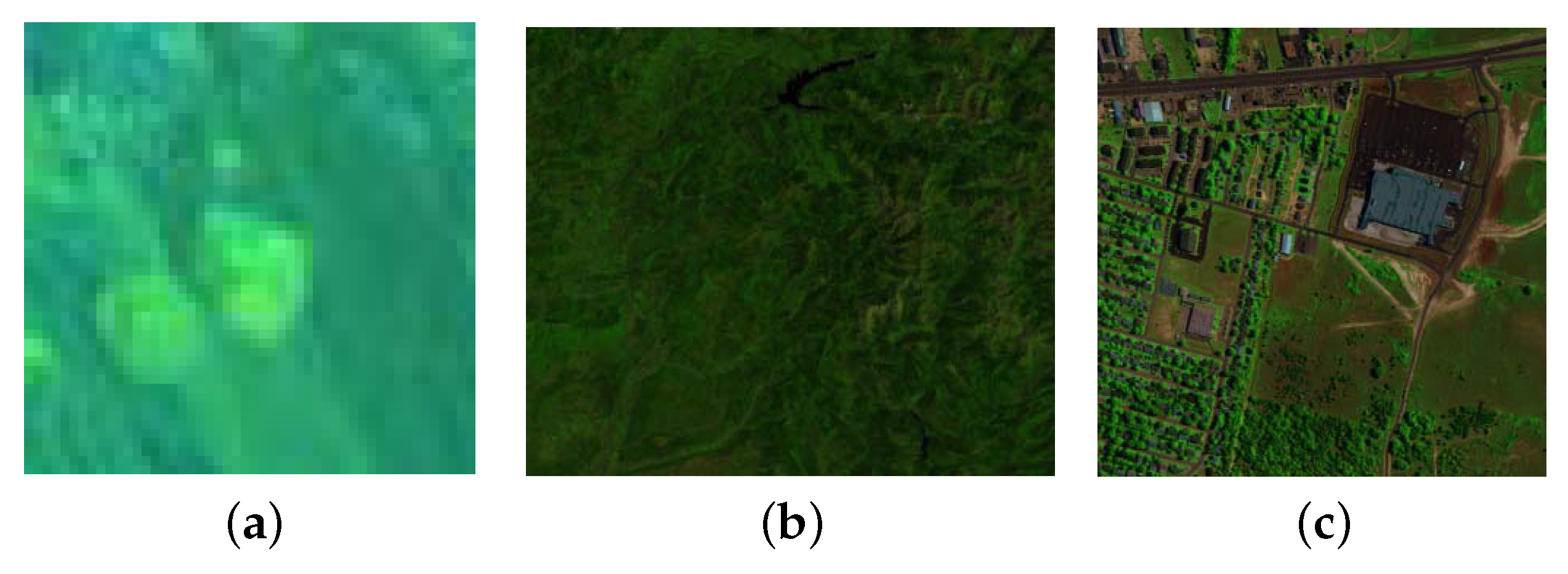
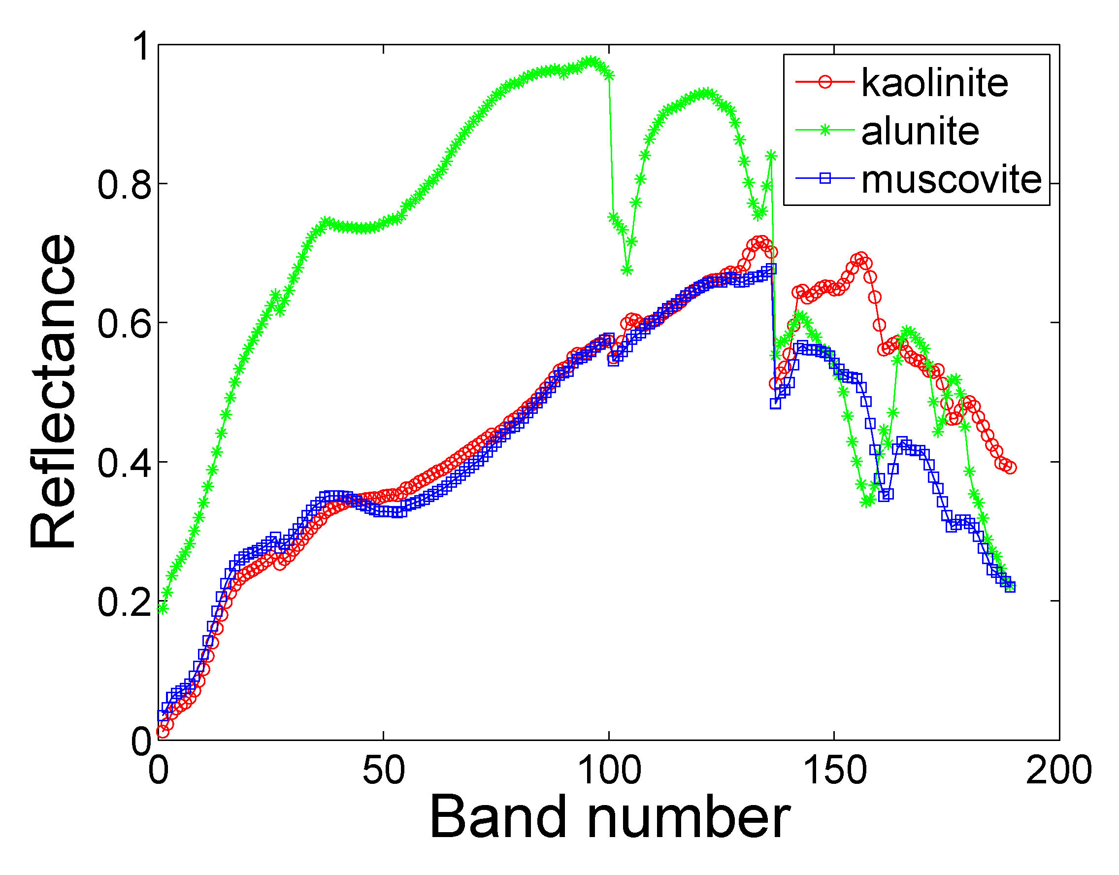
The first real HSI was acquired by the Airborne Visible Infrared Imaging Spectrometer (AVIRIS) over the Cuprite mining site, in the state of Nevada, in 1997. This HSI has 224 spectral bands ranging from 0.4 m to 2.5 m, and the spectral resolution is about 10 nm. The region of interest, containing 50 × 50 pixels, is used to assess the unmixing performance of the proposed NU-BGBM and the other four compared methods. These bands seriously contaminated by water absorption and noise are removed, remaining D = 189 spectral bands. The false color image of the selected Cuprite HSI can be seen in Figure 3a. HySime [47] can be adopted to estimate the number of endmembers in the selected Cuprite HSI. Besides, according to [28], the selected Cuprite HSI mainly has three materials, i.e., alunite, kolinite and muscovite.
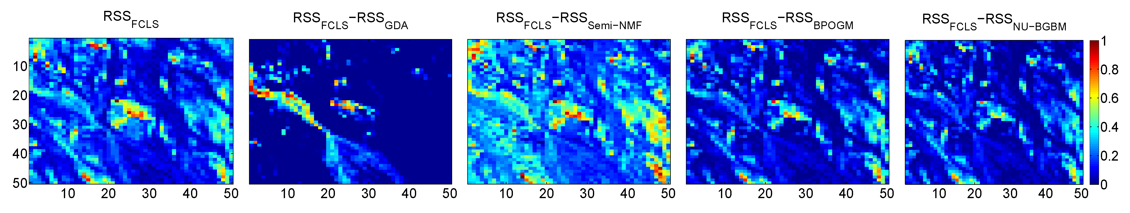
For the unmixing of real HSI, GBM and BGBM based HSI unmixing usually uses the two-stage methods. First, endmembers are extracted from the real HSI by endmember extraction methods, and the bilinear endmembers can be naturally obtained from the extracted endmembers. Then, the abundances and bilinear abundances can be estimated by different abundance estimation methods. In this experiment, we adopt the vertex component analysis (VCA) [50] to extract endmembers from the selected Cuprite HSI first, then we estimate the abundances by the proposed NU-BGBM and the other compared methods. The extracted endmembers of the selected Cuprite HSI can be seen in Figure 4. Since the truth abundances are unknown for the real HSI, and we cannot compute the RMSE, so we use the abundance maps to analyze the unmixing performance of different methods qualitatively, and also adopt the reconstruction error (RE) and spectral mean angle distance (SMAD) [30,31] to evaluate the unmixing performance of different methods quantitatively. Figure 5 shows the abundance maps estimated by the proposed NU-BGBM and the other four compared methods for the selected real Cuprite HSI. It can be observed from Figure 5 that the abundance maps, estimated by the proposed NU-BGBM and the other four compared methods for the selected real Cuprite HSI, are fairly in accordance with each other. Table 2 gives the REs and SMADs of the proposed NU-BGBM and the other four compared methods for the first real HSI. It can be clearly seen from Table 2 that the proposed NU-BGBM can obtain better RE and SMAD than the other four compared methods, which demonstrate that the proposed NU-BGBM is efficient for the unmixing of the selected real Cuprite HSI by taking the mixed noise into account. Besides, the unmixing method based on the BGBM can obtain better RE and SMAD than these unmixing methods based on the LMM and GBM, which indicate that the BGBM is more suited for the selected real Cuprite HSI than the LMM and GBM. Moreover, to demonstrate the necessity of taking the nonlinear mixing effect into consideration, the root-sum-square (RSS) [30,31] method is adopted to calculate the residual errors of HSI unmixing for each pixel. Figure 6 displays the RSS maps of FCLS for the selected real Cuprite HSI, and the difference RSS maps between FCLS and GDA, semi-NMF, BPOGM, and NU-BGBM respectively. From Figure 6, it can be observed that taking the nonlinear mixing effect into consideration can better approximate to the selected real Cuprite HSI, which demonstrate that the selected real Cuprite HSI can be better characterized by nonlinear mixtures of endmembers.
The second real HSI was acquired by the Meris spectrometer over the gulf of Lion, in the south east of France. This HSI has 13 spectral bands ranging from 400 nm to 800 nm, and the spatial resolution is 300 m. The region of interest, containing 280 × 330 pixels, is used to assess the unmixing performance of the proposed NU-BGBM and the other four compared methods. The false color image of the gulf of Lion HSI can be seen in Figure 3b. HySime [47] can be also adopted to estimate the number of endmembers for the gulf of Lion HSI. Besides, according to [24], the selected Cuprite HSI mainly has three materials, i.e., water, agricultural areas, and forests and semi natural areas. Moreover, the Corine Land Cover classification map of gulf of Lion HSI is shown in the first row of Figure 7, which can be used as potential visual ground truth to to interpret and evaluate the unmixing performance of different methods.
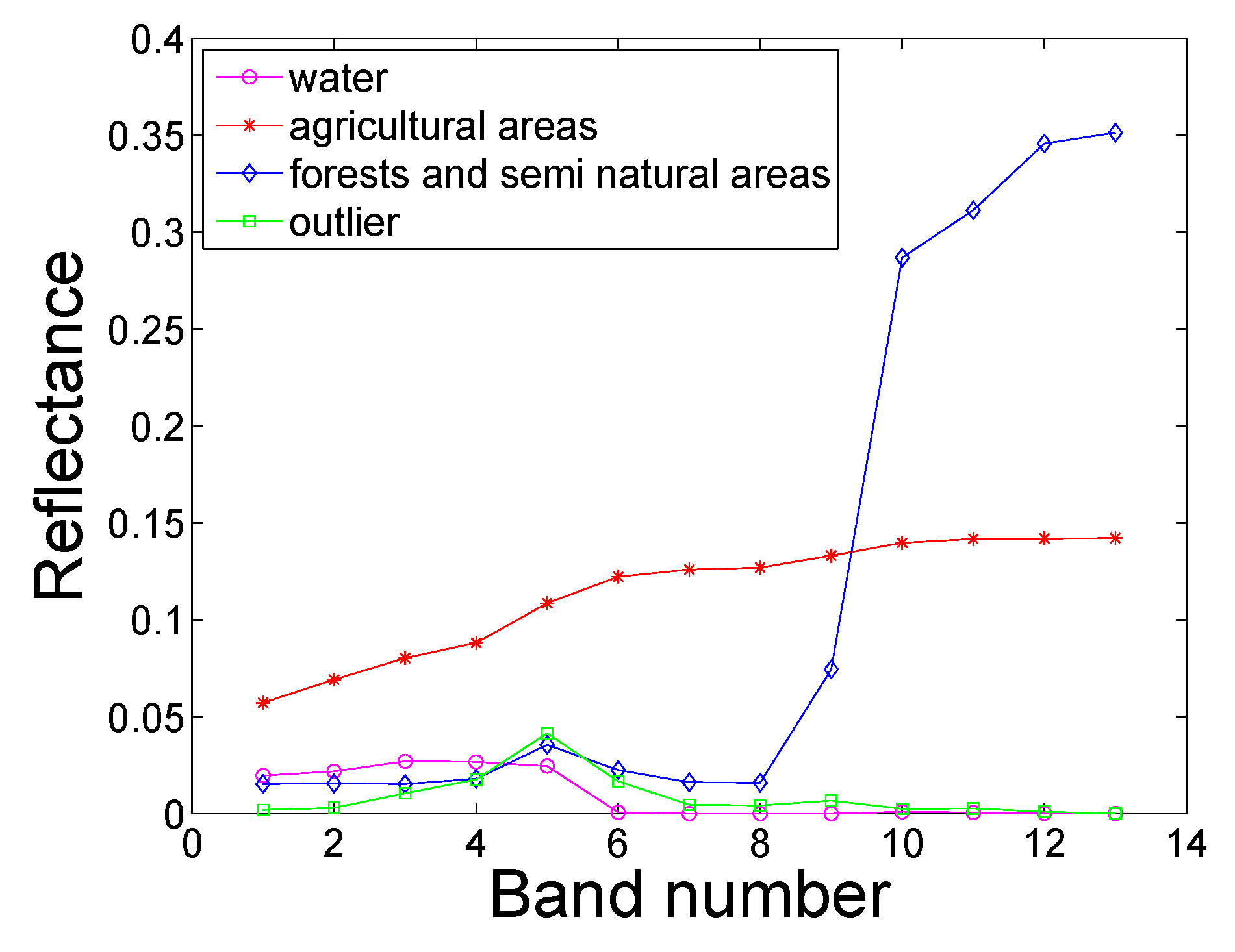
In this experiment, we also adopt the VCA [50] to extract endmembers from the gulf of Lion HSI first. However, when the number of extracted endmembers is three, one extracted endmember is not meaningful, which is due to that the corresponding abundance map is not spatially coherent. When the number of extracted endmembers is four, the three abundance maps of the meaningful endmembers are all spatially coherent, and the meaningless endmember is the outlier, which is shown in Figure 8. Figure 7 shows the abundance maps obtained by the proposed NU-BGBM and the compared methods for the gulf of Lion HSI. It can be seen from Figure 7 that the abundances of forests and semi natural areas obtained by different methods are fairly consistent with each other, and the abundances of water and agricultural areas of the proposed NU-BGBM approximate to the estimated visual ground truth better than these of the other four compared methods, which demonstrate the efficiency of the proposed method. Table 3 gives the REs and SMADs of the proposed NU-BGBM and the other four compared methods for gulf of Lion HSI. It can be observed from Table 3 that the proposed NU-BGBM can obtain better RE and SMAD than the other four compared methods, which demonstrate that the efficiency and advantages of the proposed NU-BGBM by taking the mixed noise into account. Besides, the unmixing method based on the BGBM all get smaller RE and SMAD than these unmixing methods based on the LMM and GBM, which demonstrate that the BGBM can better characterize the gulf of Lion HSI than the LMM and BGBM. Moreover, Figure 9 displays the RSS maps of FCLS for the gulf of Lion HSI, and the difference RSS maps between FCLS and GDA, semi-NMF, BPOGM, and NU-BGBM respectively. From Figure 9, it can be also clearly seen that unmixing the real HSI based on the GBM and BGBM can better approximate to the gulf of Lion HSI, which indicates that the gulf of Lion HSI is composed of nonlinear mixtures of endmembers.
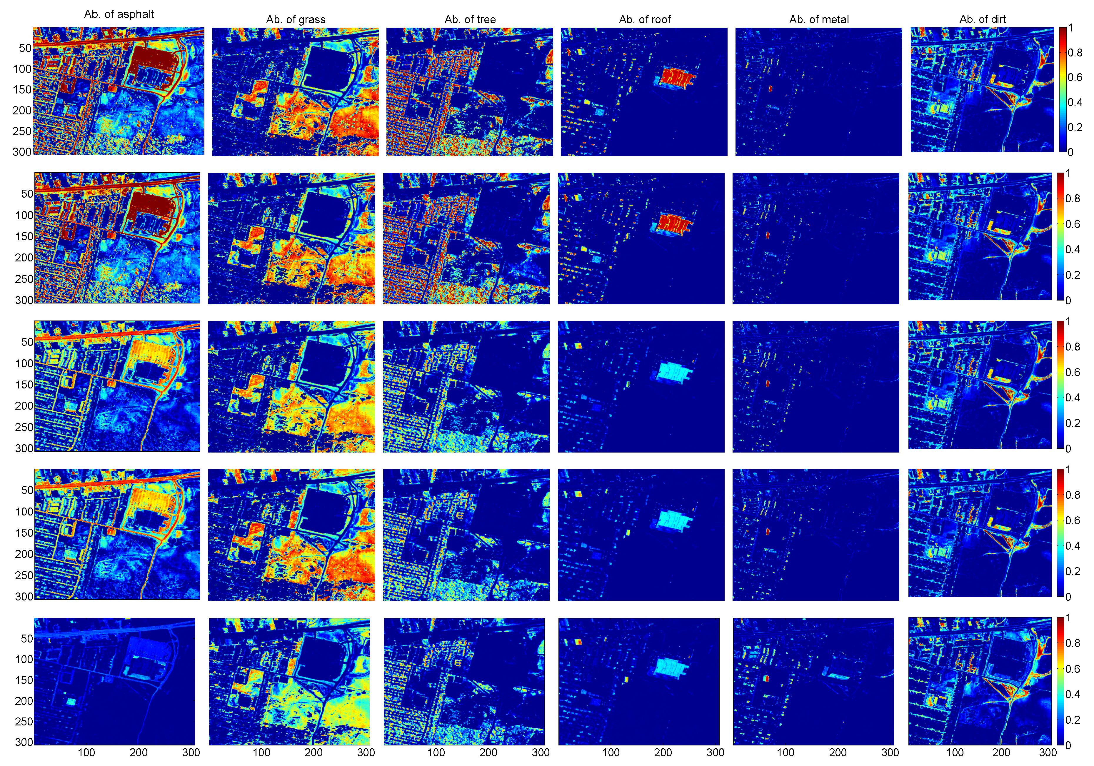
The third real HSI is the Urban data (available at: http://www.escience.cn/people/feiyunZHU/Dataset_GT.html) acquired by the Hyperspectral Digital Imagery Collection Experiment (HYDICE) over the Copperas Cove near Fort Hood. This HSI has 210 spectral bands ranging from 400 nm to 2500 nm, and the spectral resolution is 10 nm. There are 307 × 307 pixels, and the spatial resolution is 2 m. We have removed bands 1–4, 76, 87, 101–111, 136–153 and 198–210 due to water vapor and atmospheric effects, remaining D = 162 spectral bands. The false color image of the Urban data can be seen in Figure 3c. This HSI mainly has six materials, i.e., asphalt, grass, tree, roof, metal and dirt, which can be observed in Figure 10.
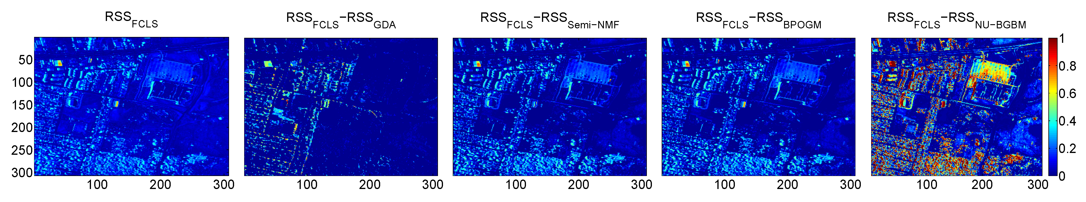
Figure 11 shows the abundance maps obtained by the proposed NU-BGBM and the compared methods for the Urban HSI. It can be observed from Figure 11 that the abundances of metal and dirt obtained by different methods are fairly consistent with each other, the abundances of tree and roof obtained by semi-NMF, BPOGM, and NU-BGBM are different from these of FCLS and GDA, the abundances of asphalt and grass obtained by NU-BGBM are different from these of FCLS, GDA, semi-NMF and BPOGM. Besides, Figure 12 displays the RSS maps of FCLS for the Urban HSI, and the difference RSS maps between FCLS and GDA, semi-NMF, BPOGM, and NU-BGBM respectively. It can be observed from Figure 12 that it helps to approximate to the Urban HSI by taking the nonlinear mixing effect into consideration. Moreover, Table 4 shows the REs and SMADs of the proposed NU-BGBM and the other four compared methods for the Urban HSI. It can be observed from Table 4 that the proposed NU-BGBM can obtain the best RE and SMAD, which demonstrate that the advantages of taking the mixed noise and different intensities of AWGN in different bands into account.
4. Conclusions
In this paper, we propose a novel nonlinear unmixing method based on the bandwise generalized bilinear model under the maximum a posteriori framework, which can take the complex mixed noise and different intensities of AWGN in different bands into consideration. Besides, we develop the ADMM to solve the proposed NU-BGBM. In the synthetic data experiments, the proposed NU-BGBM can handle the mixed noise and different intensities of AWGN much better than the other compared methods, thus our method is more robust and applicable than the other compared methods in the presence of complex mixed noise. In the real data experiments, the proposed unmixing method based on the BGBM all can get smaller RE and SMAD than these unmixing methods based on the LMM and GBM, which demonstrate that the BGBM can better characterize the selected real Cuprite HSI, gulf of Lion HSI and Urban HSI than the LMM and GBM. The proposed NU-BGBM can obtain better unmixing performance than the other four compared methods on both synthetic datasets and real HSIs, which demonstrate the effectiveness and advantages of the proposed model BGBM and the corresponding unmixing method NU-BGBM.
Although the proposed NU-BGBM can obtain desirable performance for hyperspectral unmixing, there is still room for improvement. Since the spectral signatures of neighboring pixels usually have high correlation, so we can take it into consideration to further improve the unmixing performance in out future work.
Author Contributions
All authors have made great contributions to the work. C.L., Y.L. and J.C. designed the research and analyzed the results. C.L., R.S., H.P. and Q.C. performed the experiments and wrote the manuscript. X.C. gave insightful suggestions to the work and revised the manuscript.
Funding
This research was funded by National Key R&D Program of China under grant 2017YFB1002802, the National Natural Science Foundation of China under Grants 61701160, 81571760 and 61501164, the Provincial Natural Science Foundation of Anhui under Grant 1808085QF186, and the Fundamental Research Funds for the Central Universities under Grants JZ2017HGTB0193 and JZ2018HGTB0228.
Conflicts of Interest
The authors declare no conflict of interest.
References
- Bioucas-Dias, J.M.; Plaza, A.; Dobigeon, N.; Parente, M.; Du, Q.; Gader, P.; Chanussot, J. Hyperspectral unmixing overview: Geometrical, statistical, and sparse regression-based approaches. IEEE J. Select. Top. Appl. Earth Obs. Remote Sens. 2012, 5, 354–379. [Google Scholar] [CrossRef]
- Zhang, X.; Li, C.; Zhang, J.; Chen, Q.; Feng, J.; Jiao, L.; Zhou, H. Hyperspectral unmixing via low-rank representation with space consistency constraint and spectral library pruning. Remote Sens. 2018, 10, 339. [Google Scholar] [CrossRef]
- Li, C.; Ma, Y.; Mei, X.; Fan, F.; Huang, J.; Ma, J. Sparse unmixing of hyperspectral data with noise level estimation. Remote Sens. 2017, 9, 1166. [Google Scholar] [CrossRef]
- Zhang, Z.; Liao, S.; Zhang, H.; Wang, S.; Wang, Y. Bilateral Filter Regularized L2 Sparse Nonnegative Matrix Factorization for Hyperspectral Unmixing. Remote Sens. 2018, 10, 816. [Google Scholar] [CrossRef]
- Yang, B.; Wang, B.; Wu, Z. Unsupervised Nonlinear Hyperspectral Unmixing Based on Bilinear Mixture Models via Geometric Projection and Constrained Nonnegative Matrix Factorization. Remote Sens. 2018, 10, 801. [Google Scholar] [CrossRef]
- Li, C.; Ma, Y.; Mei, X.; Liu, C.; Ma, J. Hyperspectral unmixing with robust collaborative sparse regression. Remote Sens. 2016, 8, 588. [Google Scholar] [CrossRef]
- Manolakis, D.; Siracusa, C.; Shaw, G. Hyperspectral subpixel target detection using the linear mixing model. IEEE Trans. Geosci. Remote Sens. 2001, 39, 1392–1409. [Google Scholar] [CrossRef]
- Xu, X.; Zhong, Y.; Zhang, L.; Zhang, H. Sub-pixel mapping based on a MAP model with multiple shifted hyperspectral imagery. IEEE J. Select. Top. Appl. Earth Obs. Remote Sens. 2013, 6, 580–593. [Google Scholar] [CrossRef]
- Jiang, J.; Ma, J.; Chen, C.; Wang, Z.; Wang, L. SuperPCA: A Superpixelwise Principal Component Analysis Approach for Unsupervised Feature Extraction of Hyperspectral Imagery. IEEE Trans. Geosci. Remote Sens. 2018, 56, 4581–4593. [Google Scholar] [CrossRef]
- Ma, Y.; Li, C.; Li, H.; Mei, X.; Ma, J. Hyperspectral Image Classification with Discriminative Kernel Collaborative Representation and Tikhonov Regularization. IEEE Geosci. Remote Sens. Lett. 2018, 15, 587–591. [Google Scholar] [CrossRef]
- Liu, T.; Liu, H.; Chen, Z.; Lesgold, A.M. Fast blind instrument function estimation method for industrial infrared spectrometers. IEEE Trans. Ind. Inform. 2018. [Google Scholar] [CrossRef]
- Liu, H.; Li, Y.; Zhang, Z.; Liu, S.; Liu, T. Blind Poissonian reconstruction algorithm via curvelet regularization for an FTIR spectrometer. Opt. Express 2018, 26, 22837–22856. [Google Scholar] [CrossRef] [PubMed]
- Ma, J.; Zhou, H.; Zhao, J.; Gao, Y.; Jiang, J.; Tian, J. Robust feature matching for remote sensing image registration via locally linear transforming. IEEE Trans. Geosci. Remote Sens. 2015, 53, 6469–6481. [Google Scholar] [CrossRef]
- Ma, J.; Jiang, J.; Zhou, H.; Zhao, J.; Guo, X. Guided locality preserving feature matching for remote sensing image registration. IEEE Trans. Geosci. Remote Sens. 2018, 56, 4435–4447. [Google Scholar] [CrossRef]
- Yan, J.; Li, C.; Li, Y.; Cao, G. Adaptive discrete hypergraph matching. IEEE Trans. Cybern. 2018, 48, 765–779. [Google Scholar] [CrossRef] [PubMed]
- Ghamisi, P.; Yokoya, N.; Li, J.; Liao, W.; Liu, S.; Plaza, J.; Rasti, B.; Plaza, A. Advances in hyperspectral image and signal processing: A comprehensive overview of the state of the art. IEEE Geosci. Remote Sens. Mag. 2017, 5, 37–78. [Google Scholar] [CrossRef]
- Ma, Y.; Li, C.; Mei, X.; Liu, C.; Ma, J. Robust Sparse Hyperspectral Unmixing with ℓ2,1 Norm. IEEE Trans. Geosci. Remote Sens. 2017, 55, 1227–1239. [Google Scholar] [CrossRef]
- Heylen, R.; Parente, M.; Gader, P. A review of nonlinear hyperspectral unmixing methods. IEEE J. Sel. Top. Appl. Earth Observ. Remote Sens. 2014, 7, 1844–1868. [Google Scholar] [CrossRef]
- Feng, R.; Zhong, Y.; Wang, L.; Lin, W. Rolling Guidance Based Scale-Aware Spatial Sparse Unmixing for Hyperspectral Remote Sensing Imagery. Remote Sens. 2017, 9, 1218. [Google Scholar] [CrossRef]
- Halimi, A.; Bioucas-Dias, J.M.; Dobigeon, N.; Buller, G.S.; McLaughlin, S. Fast hyperspectral unmixing in presence of nonlinearity or mismodeling effects. IEEE Trans. Comput. Imaging 2017, 3, 146–159. [Google Scholar] [CrossRef]
- Dobigeon, N.; Tourneret, J.Y.; Richard, C.; Bermudez, J.; Mclaughlin, S.; Hero, A.O. Nonlinear unmixing of hyperspectral images: Models and algorithms. IEEE. Signal Process. Mag. 2014, 31, 82–94. [Google Scholar] [CrossRef]
- Altmann, Y.; Halimi, A.; Dobigeon, N.; Tourneret, J.Y. Supervised nonlinear spectral unmixing using a postnonlinear mixing model for hyperspectral imagery. IEEE Trans. Image Process. 2012, 21, 3017–3025. [Google Scholar] [CrossRef] [PubMed] [Green Version]
- Licciardi, G.A.; Del Frate, F. Pixel unmixing in hyperspectral data by means of neural networks. IEEE Trans. Geosci. Remote Sens. 2011, 49, 4163–4172. [Google Scholar] [CrossRef]
- Ammanouil, R.; Ferrari, A.; Richard, C.; Mathieu, S. Nonlinear unmixing of hyperspectral data with vector-valued kernel functions. IEEE Trans. Image Process. 2017, 26, 340–354. [Google Scholar] [CrossRef] [PubMed]
- Hapke, B. Bidirectional reflectance spectroscopy: 1. Theory. J. Geophys. Res. Solid Earth (1978–2012) 1981, 86, 3039–3054. [Google Scholar] [CrossRef]
- Nascimento, J.M.; Bioucas-Dias, J.M. Nonlinear mixture model for hyperspectral unmixing. In Proceedings of the SPIE Image and Signal Processing Remote Sensing XV, Berlin, Germany, 31 August–3 September 2009; Bruzzone, L., Notarnicola, C., Posa, F., Eds.; SPIE: Berlin, Germany, 2009; Volume 7477, p. 74770I. [Google Scholar]
- Fan, W.; Hu, B.; Miller, J.; Li, M. Comparative study between a new nonlinear model and common linear model for analysing laboratory simulated-forest hyperspectral data. Int. J. Remote Sens. 2009, 30, 2951–2962. [Google Scholar] [CrossRef]
- Halimi, A.; Altmann, Y.; Dobigeon, N.; Tourneret, J.Y. Nonlinear unmixing of hyperspectral images using a generalized bilinear model. IEEE Trans. Geosci. Remote Sens. 2011, 49, 4153–4162. [Google Scholar] [CrossRef] [Green Version]
- Halimi, A.; Altmann, Y.; Dobigeon, N.; Tourneret, J.Y. Unmixing hyperspectral images using the generalized bilinear model. In Proceedings of the 2011 IEEE International Geoscience and Remote Sensing Symposium (IGARSS), Vancouver, BC, Canada, 24–29 July 2011; pp. 1886–1889. [Google Scholar]
- Yokoya, N.; Chanussot, J.; Iwasaki, A. Nonlinear unmixing of hyperspectral data using semi-nonnegative matrix factorization. IEEE Trans. Geosci. Remote Sens. 2014, 52, 1430–1437. [Google Scholar] [CrossRef]
- Li, C.; Ma, Y.; Huang, J.; Mei, X.; Liu, C.; Ma, J. GBM-Based Unmixing of Hyperspectral Data Using Bound Projected Optimal Gradient Method. IEEE Geosci. Remote Sens. Lett. 2016, 13, 952–956. [Google Scholar] [CrossRef]
- Yang, B.; Wang, B.; Wu, Z. Nonlinear hyperspectral unmixing based on geometric characteristics of bilinear mixture models. IEEE Trans. Geosci. Remote Sens. 2018, 56, 694–714. [Google Scholar] [CrossRef]
- Mei, X.; Ma, Y.; Li, C.; Fan, F.; Huang, J.; Ma, J. Robust GBM hyperspectral image unmixing with superpixel segmentation based low rank and sparse representation. Neurocomputing 2018, 275, 2783–2797. [Google Scholar] [CrossRef]
- Heylen, R.; Scheunders, P. A multilinear mixing model for nonlinear spectral unmixing. IEEE Trans. Geosci. Remote Sens. 2016, 54, 240–251. [Google Scholar] [CrossRef]
- Wei, Q.; Chen, M.; Tourneret, J.Y.; Godsill, S. Unsupervised nonlinear spectral unmixing based on a multilinear mixing model. IEEE Trans. Geosci. Remote Sens. 2017, 55, 4534–4544. [Google Scholar] [CrossRef]
- Yang, B.; Wang, B. Band-Wise Nonlinear Unmixing for Hyperspectral Imagery Using an Extended Multilinear Mixing Model. IEEE Trans. Geosci. Remote Sens. 2018, 99, 1–16. [Google Scholar] [CrossRef]
- Zhang, H.; He, W.; Zhang, L.; Shen, H.; Yuan, Q. Hyperspectral image restoration using low-rank matrix recovery. IEEE Trans. Geosci. Remote Sens. 2014, 52, 4729–4743. [Google Scholar] [CrossRef]
- Li, C.; Ma, Y.; Huang, J.; Mei, X.; Ma, J. Hyperspectral image denoising using the robust low-rank tensor recovery. J. Opt. Soc. Am. A Opt. Image Sci. Vis. 2015, 32, 1604–1612. [Google Scholar] [CrossRef] [PubMed]
- Fan, F.; Ma, Y.; Li, C.; Mei, X.; Huang, J.; Ma, J. Hyperspectral image denoising with superpixel segmentation and low-rank representation. Inf. Sci. 2017, 397, 48–68. [Google Scholar] [CrossRef]
- Fan, H.; Li, C.; Guo, Y.; Kuang, G.; Ma, J. Spatial-Spectral Total Variation Regularized Low-Rank Tensor Decomposition for Hyperspectral Image Denoising. IEEE Trans. Geosci. Remote Sens. 2018, 56, 6196–6213. [Google Scholar] [CrossRef]
- Aggarwal, H.K.; Majumdar, A. Hyperspectral unmixing in the presence of mixed noise using joint-sparsity and total variation. IEEE J. Select. Top. Appl. Earth Obs. Remote Sens. 2016, 9, 4257–4266. [Google Scholar] [CrossRef]
- Boyd, S.; Parikh, N.; Chu, E.; Peleato, B.; Eckstein, J. Distributed optimization and statistical learning via the alternating direction method of multipliers. Found. Trends Mach. Learn. 2011, 3, 1–122. [Google Scholar] [CrossRef]
- Iordache, M.D.; Bioucas-Dias, J.M.; Plaza, A. Sparse unmixing of hyperspectral data. IEEE Trans. Geosci. Remote Sens. 2011, 49, 2014–2039. [Google Scholar] [CrossRef]
- Qu, Q.; Nasrabadi, N.M.; Tran, T.D. Abundance estimation for bilinear mixture models via joint sparse and low-rank representation. IEEE Trans. Geosci. Remote Sens. 2014, 52, 4404–4423. [Google Scholar]
- Zhu, F.; Halimi, A.; Honeine, P.; Chen, B.; Zheng, N. Correntropy Maximization via ADMM: Application to Robust Hyperspectral Unmixing. IEEE Trans. Geosci. Remote Sens. 2017, 55, 4944–4955. [Google Scholar] [CrossRef] [Green Version]
- Donoho, D.L. De-noising by soft-thresholding. IEEE Trans. Inf. Theory 1995, 41, 613–627. [Google Scholar] [CrossRef] [Green Version]
- Bioucas-Dias, J.M.; Nascimento, J.M. Hyperspectral subspace identification. IEEE Trans. Geosci. Remote Sens. 2008, 46, 2435–2445. [Google Scholar] [CrossRef]
- Heinz, D.C.; Chang, C.I. Fully constrained least squares linear spectral mixture analysis method for material quantification in hyperspectral imagery. IEEE Trans. Geosci. Remote Sens. 2001, 39, 529–545. [Google Scholar] [CrossRef]
- Miao, L.; Qi, H. Endmember extraction from highly mixed data using minimum volume constrained nonnegative matrix factorization. IEEE Trans. Geosci. Remote Sens. 2007, 45, 765–777. [Google Scholar] [CrossRef]
- Nascimento, J.M.; Dias, J.M.B. Vertex component analysis: A fast algorithm to unmix hyperspectral data. IEEE Trans. Geosci. Remote Sens. 2005, 43, 898–910. [Google Scholar] [CrossRef]
Figure 1.
Six selected spectra in the USGS.
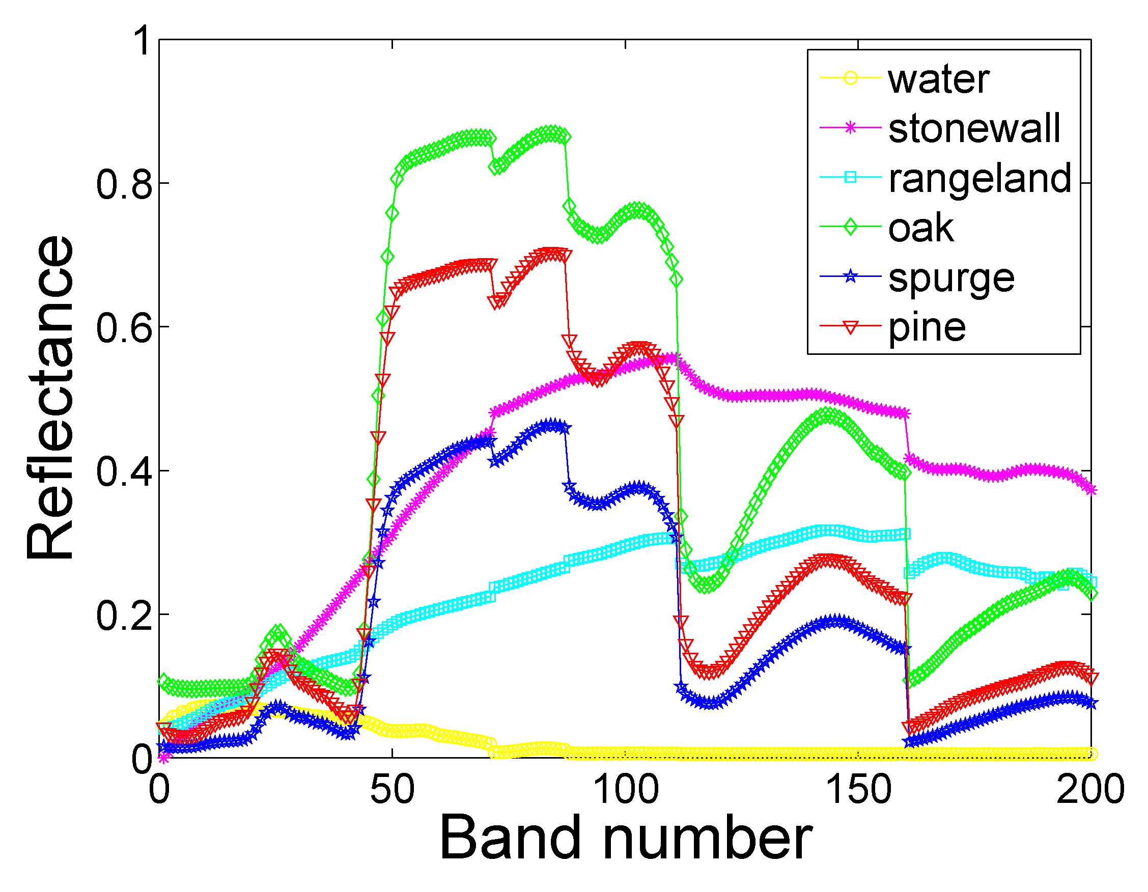
Figure 2.
Abundance maps estimated by the compared methods and the proposed method in the presence of three types of noise. From top to bottom: ground truth, FCLS, GDA, semi-NMF, BPOGM and NU-BGBM.
Figure 2.
Abundance maps estimated by the compared methods and the proposed method in the presence of three types of noise. From top to bottom: ground truth, FCLS, GDA, semi-NMF, BPOGM and NU-BGBM.
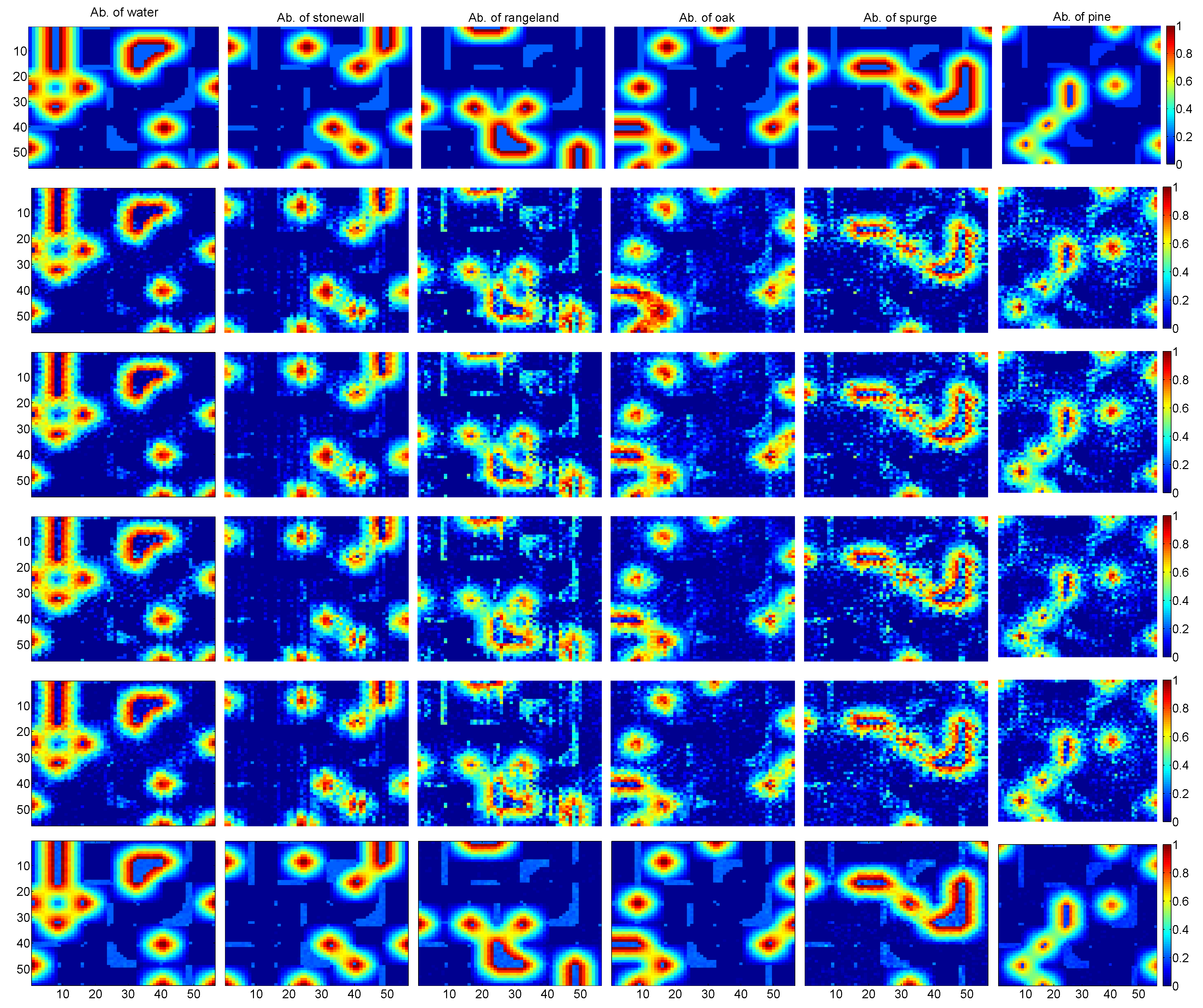
Figure 3.
False-color image of (a) Cuprite, (b) gulf of Lion and (c) Urban.

Figure 4.
Extracted endmembers of Cuprite.

Figure 5.
Abundance maps estimated by the proposed NU-BGBM and the compared methods for the selected real Cuprite HSI. From top to bottom: FCLS, GDA, semi-NMF, BPOGM, and NU-BGBM.
Figure 5.
Abundance maps estimated by the proposed NU-BGBM and the compared methods for the selected real Cuprite HSI. From top to bottom: FCLS, GDA, semi-NMF, BPOGM, and NU-BGBM.
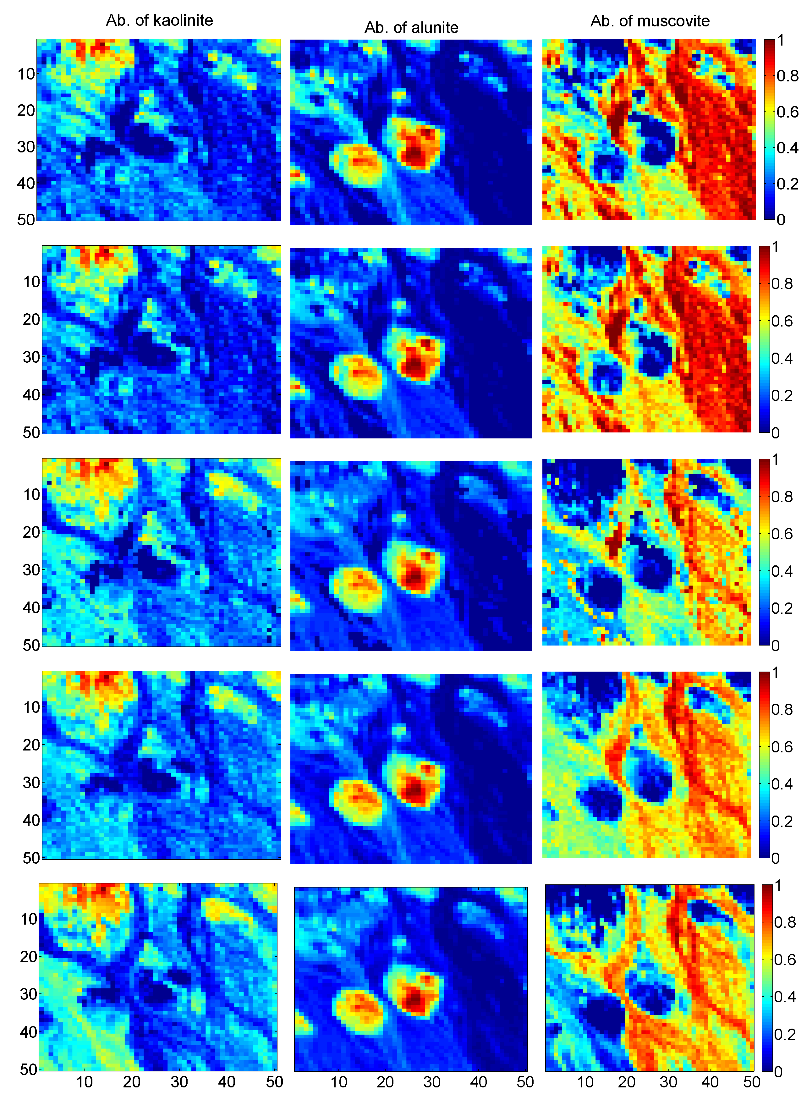
Figure 6.
RSS maps of FCLS for the selected real Cuprite HSI, and the difference RSS maps between FCLS and GDA, semi-NMF, BPOGM, and NU-BGBM respectively.
Figure 6.
RSS maps of FCLS for the selected real Cuprite HSI, and the difference RSS maps between FCLS and GDA, semi-NMF, BPOGM, and NU-BGBM respectively.

Figure 7.
Abundance maps estimated by the proposed NU-BGBM and the compared methods for the gulf of Lion real HSI. From top to bottom: estimated visual ground truth, FCLS, GDA, semi-NMF, BPOGM, and NU-BGBM.
Figure 7.
Abundance maps estimated by the proposed NU-BGBM and the compared methods for the gulf of Lion real HSI. From top to bottom: estimated visual ground truth, FCLS, GDA, semi-NMF, BPOGM, and NU-BGBM.
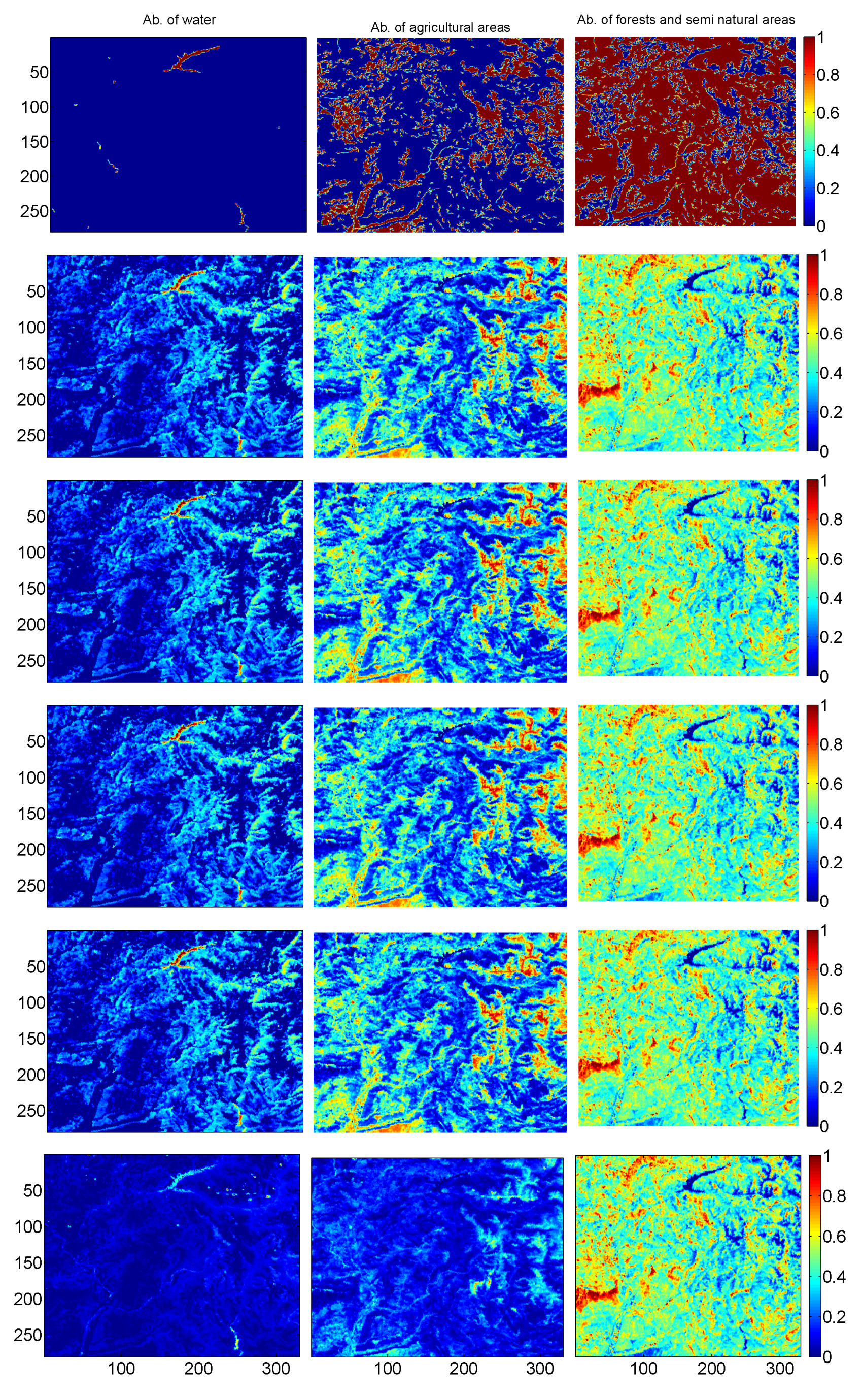
Figure 8.
Extracted endmembers of gulf of Lion.

Figure 9.
RSS maps of FCLS for the gulf of Lion real HSI, and the difference RSS maps between FCLS and GDA, semi-NMF, BPOGM, and NU-BGBM respectively.
Figure 9.
RSS maps of FCLS for the gulf of Lion real HSI, and the difference RSS maps between FCLS and GDA, semi-NMF, BPOGM, and NU-BGBM respectively.
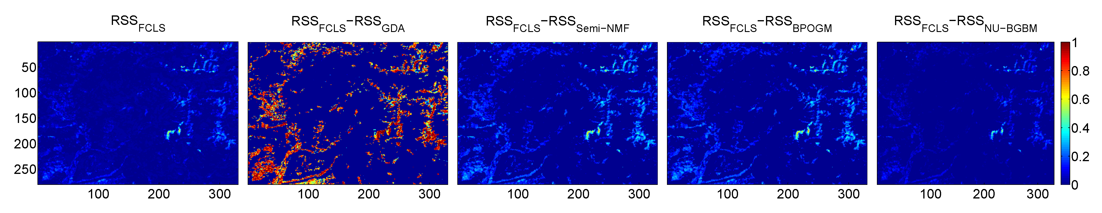
Figure 10.
Endmembers of Urban.
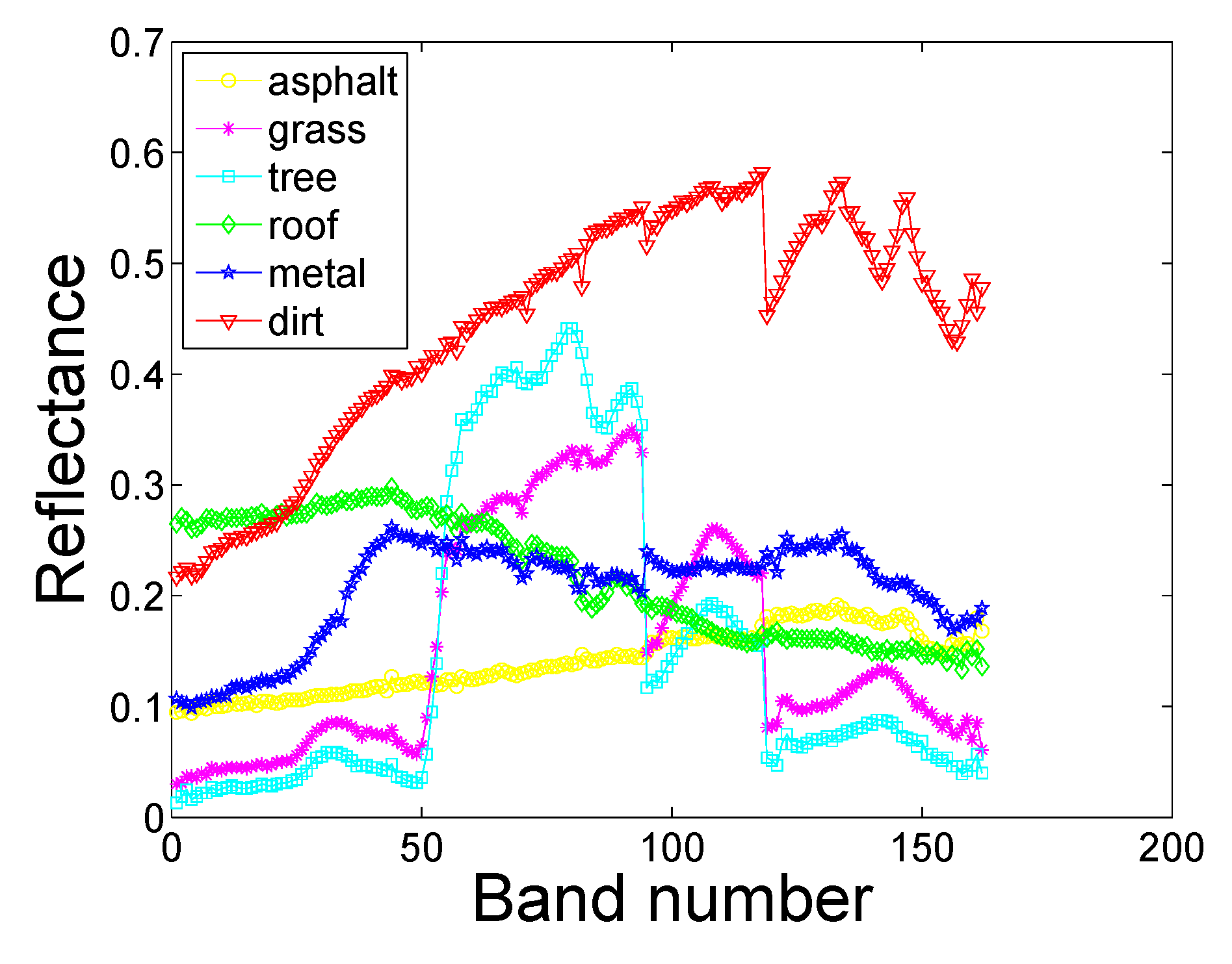
Figure 11.
Abundance maps estimated by the proposed NU-BGBM and the compared methods for the Urban real HSI. From top to bottom: estimated visual ground truth, FCLS, GDA, semi-NMF, BPOGM, and NU-BGBM.
Figure 11.
Abundance maps estimated by the proposed NU-BGBM and the compared methods for the Urban real HSI. From top to bottom: estimated visual ground truth, FCLS, GDA, semi-NMF, BPOGM, and NU-BGBM.

Figure 12.
RSS maps of FCLS for the Urban real HSI, and the difference RSS maps between FCLS and GDA, semi-NMF, BPOGM, and NU-BGBM respectively.
Figure 12.
RSS maps of FCLS for the Urban real HSI, and the difference RSS maps between FCLS and GDA, semi-NMF, BPOGM, and NU-BGBM respectively.

Table 1.
Comparison of RMSEs () for different methods in the presence of different types of noise.
| Type of Noise | FCLS | GDA | Semi-NMF | BPOGM | NU-BGBM |
|---|---|---|---|---|---|
| Gaussian noise | 7.103 | 6.053 | 5.520 | 5.157 | 0.990 |
| Impulse noise | 7.123 | 6.395 | 6.161 | 5.403 | 0.167 |
| Dead lines | 6.812 | 5.773 | 5.796 | 5.436 | 0.171 |
| Gaussian noise & Impulse noise | 8.411 | 7.781 | 7.651 | 7.065 | 1.004 |
| Gaussian noise & Dead lines | 8.084 | 7.185 | 7.197 | 6.996 | 1.003 |
| Impulse noise & Dead lines | 7.941 | 7.254 | 7.469 | 6.962 | 0.296 |
| Gaussian noise & Impulse noise & Dead lines | 9.010 | 8.395 | 8.609 | 8.216 | 1.021 |
Table 2.
Comparison of REs () and SMADs () of different methods using extracted endmembers for the selected Cuprite real HSI.
Table 2.
Comparison of REs () and SMADs () of different methods using extracted endmembers for the selected Cuprite real HSI.
| FCLS | GDA | Semi-NMF | BPOGM | NU-BGBM | |
|---|---|---|---|---|---|
| RE | 2.106 | 1.980 | 1.481 | 1.117 | 1.046 |
| SMAD | 3.131 | 2.920 | 2.738 | 2.077 | 1.891 |
Table 3.
Comparison of REs () and SMADs () of different methods using extracted endmembers for the gulf of lion real HSI.
Table 3.
Comparison of REs () and SMADs () of different methods using extracted endmembers for the gulf of lion real HSI.
| FCLS | GDA | Semi-NMF | BPOGM | NU-BGBM | |
|---|---|---|---|---|---|
| RE | 1.138 | 1.044 | 0.899 | 0.898 | 0.353 |
| SMAD | 3.932 | 3.660 | 3.585 | 3.581 | 2.643 |
Table 4.
Comparison of REs () and SMADs () of different methods using extracted endmembers for the Urban real HSI.
Table 4.
Comparison of REs () and SMADs () of different methods using extracted endmembers for the Urban real HSI.
| FCLS | GDA | Semi-NMF | BPOGM | NU-BGBM | |
|---|---|---|---|---|---|
| RE | 4.120 | 4.057 | 1.837 | 1.721 | 1.443 |
| SMAD | 12.713 | 12.646 | 9.541 | 9.000 | 7.353 |
© 2018 by the authors. Licensee MDPI, Basel, Switzerland. This article is an open access article distributed under the terms and conditions of the Creative Commons Attribution (CC BY) license (http://creativecommons.org/licenses/by/4.0/).
Share and Cite
MDPI and ACS Style
Li, C.; Liu, Y.; Cheng, J.; Song, R.; Peng, H.; Chen, Q.; Chen, X. Hyperspectral Unmixing with Bandwise Generalized Bilinear Model. Remote Sens. 2018, 10, 1600. https://doi.org/10.3390/rs10101600
AMA Style
Li C, Liu Y, Cheng J, Song R, Peng H, Chen Q, Chen X. Hyperspectral Unmixing with Bandwise Generalized Bilinear Model. Remote Sensing. 2018; 10(10):1600. https://doi.org/10.3390/rs10101600
Chicago/Turabian StyleLi, Chang, Yu Liu, Juan Cheng, Rencheng Song, Hu Peng, Qiang Chen, and Xun Chen. 2018. "Hyperspectral Unmixing with Bandwise Generalized Bilinear Model" Remote Sensing 10, no. 10: 1600. https://doi.org/10.3390/rs10101600
Note that from the first issue of 2016, this journal uses article numbers instead of page numbers. See further details here.