Modeling the Directional Clumping Index of Crop and Forest

Abstract

The Clumping Index (Ω) was introduced to quantify the spatial distribution pattern of vegetation elements. It is crucial to improve the estimation accuracy of vital vegetation parameters, such as Leaf Area Index (LAI) and Gross Primary Production (GPP). Meanwhile, the parameterization of Ω is challenging partly due to the varying observations of canopy gaps from different view angles. Many previous studies have shown the increase of Ω with view zenith angle through samples of gap size distribution from in situ measurements. In contrast, remote sensing retrieval algorithms only assign a constant value for each biome type to roughly correct the clumping effect as a compromise between the accuracy and efficiency. In this paper, analytical models are proposed that estimate the directional clumping index (Ω(θ)) of crop and forest at canopy level. The angular variation trend and magnitude of crop Ω(θ) was analyzed within row structure where vegetation elements are randomly spaced along rows. The forest model predicts Ω(θ) with tree density, distribution pattern, crown shape, trunk size, and leaf area and angle distribution function. The models take into account the main directional characteristics of clumping index using easy-to-measure parameters. Test cases showed that Ω(θ) magnitude variation for black spruce forest was 102.3% of the hemispherical average clumping index ($\tilde{\mathsf{\Omega }}$), whereas the Larch forest had 48.7% variation, and row crop variation reached 32.4%. This study provided tools to assess Ω(θ) of discontinuous canopies.

1. Introduction

Canopy clumping affects the gap fraction and redistributes radiation interception within the canopy [1,2,3,4]. The assumption of random distributions causes underestimation of leaf area index (LAI) as compared to considering clumping, since the clumping phenomenon of natural forest increases the gap fraction [5,6,7]. Therefore, the effective LAI that was indirectly obtained from gap fraction measurements needs to be interpreted together with the clumping condition to approach the actual LAI, i.e., the one-sided leaf area per unit horizontal ground surface area [8,9,10,11].

Clumping index (Ω) is a commonly used vegetation dispersion parameter that quantifies the level of foliage distribution non-randomness in real case [12], with Ω = 1 for completely randomly distributed foliage, Ω > 1 for regular spatially distributed foliage, and 0 < Ω < 1 for clumped foliage [13,14].

The difficulties in assigning Ω are due to its multiple scale and directional variation. First, the clumping effect exist at different scales, such as at shoot level, among canopies level, and at the ecosystem level [7,15,16,17,18,19,20]. Second, canopy level Ω varies with zenith angle so that the directional change of clumping index has attracted more and more attention [16,19,21,22,23].

Due to this complexity, the study and application of Ω faces accuracy-efficiency-robustness trade-off [19]. In field campaigns, Ω is derived from gap size statistics or gap fraction, as measured by many ground based optical instruments, such as the Tracing Radiation and Architecture of Canopies (TRAC) system [18] or fish-eye photographs [24]. In situ measured Ω can accurately depict the site-specific Ω variation, but lack efficiency. Nevertheless, it is risky to extrapolate the values or relationships beyond the site.

In operational retrieval of MODIS LAI product, the algorithm assigns a single clumping factor to each biome type [25]. This is the most simplified method but it guarantees the robustness. Chen et al. [4] developed a satellite level regression model for hemispherical average clumping index from an angular index that is called the normalized difference between hotspot and dark spot (NDHD), which made it possible to retrieve global time series average clumping index [9,26,27]. The NDHD method balances the need for computational efficiency while including the pixel specific information. However, the directional variation of clumping index has not been included.

The angular variation of directional clumping index (Ω(θ)) contains abundant vegetation structure information [28]. Discontinuous crop and forest are two representative examples. The directional variation pattern of the clumping effect reflects various vegetation canopy morphologies [29,30].

Furthermore, the directionality of clumping index is necessary to be taken into account in vegetation monitoring for two reasons. One reason is the observed clumping varies along with the view direction, which results in the uncertainty in using single clumping index value. Another reason is the accuracy of Ω estimation has an apparent influence on LAI and Gross Primary Production (GPP). Ω estimation error directly and linearly affects LAI retrievals. Normally, LAI measurements from optical instruments and sensors are referred to as effective LAI (LAI_e), the product of $\mathsf{\Omega }$ and actual LAI (LAI) (half the total leaf area) ($LA{I}_e=\mathsf{\Omega }·LAI$). Garrigues et al. [31] tested LAI retrieval sensitivity while using digital hemispherical photography over 10 crop types. The clumping index induced difference in LAI estimation at 30-m scale was as high as 31% (relative root-mean-square error or relative RMSE). Weiss [14] suggested that the accurate estimation of clumping index for each zenith angle will increase LAI estimation accuracy. Piayda et al. [32] applied angularly dependent leaf clumping index in determining LAI, which led to a 30% higher estimation when compared to the indirect measurements using LAI-2000, but matched precisely with the direct measurements using litter traps. Chen et al. [33] tested the effects of ignoring foliage clumping characteristics in global GPP mapping, and found that neglecting clumping index will increase the uncertainty in GPP estimation, particularly in tropical regions. Using accurate LAI, but ignoring clumping index, causes an overestimation of global GPP by 12%; applying the effective LAI without considering the clumping effect would underestimate global GPP by 9%. Comparing the effect of clumping index on LAI/GPP estimation and the directional variation magnitude of Ω [2,21], it is necessary to apprehend that if angular variation is not provided as well as the average, large errors can occur in the inverted leaf angle distribution and LAI for canopies with direction dependent clumping [34].

Many studies have discussed the directional variation of Ω using the gap size distribution measurements from in situ instruments, such as TRAC or digital hemispherical photography. The efficiency in data measurement is the bottleneck in wide application of the gap size distribution model. Kuusk [22] developed a simulation model that had extended the understanding of directional clumping effect, but it was difficult to be applied for practical calculations, as many input parameters cannot be measured. Kucharik [21] modeled the directional clumping index using an empirical equation to extend its availability for more species, although the accuracy of coefficients is restricted in the regression hull. This paper aims to propose analytical models to estimate directional clumping index of crop and forest at canopy level.

According to the Beer’s law [35], the clumping index can be estimated as a function of gap fraction of vegetation canopy. Crop canopy illustrates an apparent clumping index angular dependence due to its gap fraction variation in discrete periodic row structures [22,36,37]. Fan et al. [37] proposed an analytical model for the crop clumping index using the directional average gap fraction, where each hedgerow was regarded as the integration of four parts with different average LAI. This assumption led to an accurate expression of crop clumping index, although the integration component is incorrect in concept. Peng et al. [38] rectified the method and applied the directional clumping index in retrieving crop albedo. The average gap fraction of forest was estimated according to the interaction between light regime and the canopy, such as the widely used Geometric-Optical (GO) model that was proposed by Li et al. [39], Nilson [7], and Xu [40]. In the GO model, forest gap fraction is the complement of the projected area fraction on the ground. Nilson [7] proposed the gap probability was determined by the number of trunks occurring in the shadowed region of a single tree. It is assumed each tree crown was ellipsoid, which fits most practical cases. The measurements and simulations [21] suggest that the largest gaps between crowns are a major cause of the canopy clumping effect.

This paper proposed analytical models for crop and forest directional clumping index based on gap fraction estimation. To extend the applicability of the model, we emphasized the angular variation of Ω due to the first-level structure, i.e., the row structure of crop, and the abundance of crown shapes coupled with complex tree spatial distribution of forest.

Section 1 introduced the importance of clumping index and the necessity of directional clumping index according to the previous studies. Section 2 introduces the derived analytical model of angular clumping index variation for crop and forest. Section 3 demonstrates validation of the model, while using in situ results to validate the reliability of the proposed methods, and we evaluated the variation range of $\mathsf{\Omega }(\theta )$. Section 4 analyzes the influence of various parameters on directional clumping index using the proposed methods. Section 5 summarizes the main conclusion and proposes the limitations in the model and analysis. The symbols used in this paper are listed in

Table 1. List of symbols used in the clumping index (Ω) models.

Symbol	Description	Unit
$\theta$	Zenith angle, $\mu =\cos \theta$	degree
$\phi$	Azimuth angle	degree
$p$	Gap fraction	dimensionless
$\mathsf{\Omega }$	Clumping index (Ω)	dimensionless
LAI	Leaf area index	dimensionless
u	Leaf volume density	m−1
$G_{\theta }$	Mean projection of unit foliage area along the direction of zenith angle $\theta$	dimensionless
$A/A_1/A_2/H$	Row period width, row width, gap width, and crop height, respectively. $A=A_1+A_1$ for any $\phi$	m
$a_1/a_2$	Row width and gap width, respectively, in the direction perpendicular to the row	m
R	Radius of the tree crown	m
H	Height (or depth) of the tree crown	m
$d_t$	Trunk diameter at breast height, DBH	m
$h_t$	Trunk height	m
$C_{CR}$	Crown closure, counting overlapped crown projection multiple times	dimensionless
$C_{CA}$	Crown closure, counts overlapped crown projection once	dimensionless
$P$	Probability	dimensionless
N	Average number of trees in unit area	dimensionless
M	Average number of trees in a quadrat defined by the Poisson distribution	dimensionless
m1	Average group number of trees in a sample area defined by the Neyman distribution	dimensionless
m2	Average number of trees in each group	dimensionless
$\rho$	Leaf reflectance	dimensionless
$T$	Leaf transmittance	dimensionless
$r_g^h$	Bi-directional reflectance of soil	dimensionless
$r_g^d$	Directional-hemispherical reflectance of soil	dimensionless

.

2. Modeling and Evaluation

Crop Ω generally varies with azimuth angle, whereas forest Ω is generally symmetric in the azimuth dimension. Different algebraic models are firstly proposed for their respective directional clumping index estimation.

Simulation is a practical choice to validate algebraic expression. The Monte Carlo (MC) method was employed for crops [38]. The morphological statistics was proposed for forests, which quantifies the gap fraction through automatic counting that is based on virtual forest scenarios. Simulated results can capture the general variation trends of directional gap fractions and provide reference results.

2.1. Analytical Method for Crop and Forest

2.1.1. Crop Model

We regard the crop as clumps of vegetation elements at the canopy level [37]. The vegetation elements are randomly distributed within hedgerows [41]. Following the Beer’s law, the average gap fraction of the vegetation canopy is a function of view zenith angle and its structural parameters, including clumping index, LAI, and leaf angle distribution [42],

$$\overline{p(\theta ,\phi )}=\exp (-\mathsf{\Omega }(\theta ) \frac{G_{\theta }}{\mu } LA{I}_a)$$

(1)

where $\overline{p(\theta ,\phi )}$ is the gap fraction; $\mathsf{\Omega }(\theta )$ refers to the directional clumping index; $G_{\theta }$ is a parameter to describe canopy structure; μ is the cosine of zenith angle θ; and, $LA{I}_a$ denotes the spatially-averaged leaf area index.

The average gap fraction of hedgerow crop canopy can be estimated using Yan et al.’s algorithm [41].

$$\overline{p(\theta ,\phi )}=\frac{1}{A}\left[\begin{array}{l}\left(A_1-H \tan \theta -2 \frac{\sin \theta }{G_{\theta } u}\right) e^{-\frac{G_{\theta } u H}{\cos \theta }}\\ +\left(A_2-H \tan \theta +2 \frac{\sin \theta }{G_{\theta } u}\right)\end{array}\right]$$

(2)

where A is a row unit consisting of canopy width ($A_1=a_1/\sin \phi$) and row spacing ($A_2=a_2/\sin \phi$) at a relative azimuth angle of $\phi$ with the row direction; $a_1$ and $a_2$ represents the canopy width and row spacing that vertical to the row direction. H is the height of the crop. Then, $\mathsf{\Omega }(\theta )$ can be calculated from the average gap fraction, $\overline{p(\theta ,\phi )}$, i.e.,

$$\mathsf{\Omega }(\theta )=-\frac{\mu \ln \left(\overline{p(\theta ,\phi )}\right)}{G_{\theta } LA{I}_a}$$

(3)

where the equivalent LAI ($LA{I}_a$), includes the influence of foliage and non-foliage elements.

Kucharik et al. [16,21] proposed that the canopy clumping index is a function of path length through the canopy. More specifically, it is a function of the effective path length in proportion to the encountered vegetation elements, as it is related to the energy attenuation in the canopy. For crop canopy, this effective path length does not count the row gap. Therefore, the maximum effective path length shows ups and downs while penetrating more rows and row gaps at increasing zenith angles, which is illustrated as the line A–E in Figure 1.

Accordingly, the variation of $\mathsf{\Omega }(\theta )$ with zenith angle can be pinpointed while using the local feature angles, ${\theta }_{\mathrm{c}i}$, corresponding to the peaks of the $\mathsf{\Omega }(\theta )$ curve with zenith angle (Figure 2). The feature angles are determined by the row structure,

$$\begin{array}{l}{\theta }_{\mathrm{c}i}={\tan }^{-1}\left(\frac{iA}{H}\right)\\ {\theta }_{\mathrm{d}i}={\tan }^{-1}\left(\frac{iA+A_1}{H}\right)\end{array}$$

(4)

where i = 1, 2, 3, … i denotes the number of rows that photons penetrated through in the crop canopy; and $A=A_1+A_2=a_1/\sin \phi +a_2/\sin \phi$. The subscript c and d corresponds to the local peak and valley value.

Ω(θ) increases along with zenith angle before reaching the first feature angle (Figure 2). In practice, if the fluctuation (normally < 0.05) can be tolerated for Ω(θ), we can regard Ω(θ) as approximately stable after the first turning point ${\theta }_c$. Therefore, ${\theta }_c$ can be used to predict the main Ω(θ) trend, which is regarded as the range angle of Ω(θ),

$${\theta }_{\mathrm{c}}={\tan }^{-1}\left(\frac{A}{H}\right)$$

(5)

2.1.2. Forest Model

The derivation of forest Ω(θ) uses the average gap fraction (3), which is referred to Nilson’s model [7]. We modelled the tree crown as vertical ellipsoid for three reasons. First, the vertical ellipsoid is axially symmetrical, which accords with our assumption that the variation of clumping index along with azimuth angle is not considered. Second, the crowns of different species can be discriminated though the ratio between crown depth and crown width, which is related to the variation of the clumping index along with zenith angle. Third, the ellipsoid can be easily parameterized using crown depth and crown width in the model.

For randomly distributed forest, the gap fraction at canopy level can be expressed as

$$p_{\theta }=e^{-n\pi R^2 \sqrt{1+{(\frac{h}{2R})}^2 {\tan }^2\theta } (1-p_1(\theta ))}$$

(6)

where $p_i(\theta )$ is the intra-crown directional gap fraction of the tree, $h/2R$ is a crown shape factor that discriminates different trees types or species, and $n\pi R^2$ is the crown closure where the overlapped regions of crown projections have been multiply counted, i.e., $C_{CR} =n\pi R^2$. Combining (3) and (4),

$$\mathsf{\Omega }\left(\theta \right)=\frac{C_{CR}\sin \theta \sqrt{{\tan }^{-2}\theta +{(\frac{h}{2R})}^2 }\left(1-p_1(\theta )\right)}{G LA{I}_{\mathrm{a}}}$$

(7)

However, (6) and (7) do not consider the trunk, which can affect optical measurements for some high trees with tall or wide trunks [43]. The average gap fraction at canopy level, incorporating trunk effects, can be expressed as

$$p_{\theta }=e^{-n\left(\pi R^2\sqrt{1+{(\frac{h}{2R})}^2 {\tan }^2\theta }+d_t h_t \tan \theta \right) (1-p_1(\theta ))}$$

(8)

and the directional Ω(θ) can be expressed as

$$\mathsf{\Omega }\left(\theta \right)=\frac{C_{CR}\sin \theta \left(\sqrt{{\tan }^{-2}\theta +{(\frac{h}{2R})}^2}+\frac{d_t h_t}{\pi R^2}\right)\left(1-p_1(\theta )\right)}{G LA{I}_{\mathrm{a}}}$$

(9)

Alternatively, if we count the overlapped regions of crown projections only once in the canopy closure calculation, then $C_{CA}=1-e^{-n \pi R^2}$, since it is equivalent to the canopy gap fraction at the nadir direction. Then, the canopy average gap fraction and Ω(θ) can be expressed as, respectively,

$$p_{\theta }={\left(1-C_{CA}\right)}^{\sqrt{1+{(\frac{h}{2R})}^2 {\tan }^2\theta } (1-p_1(\theta ))}$$

(10)

and

$$\mathsf{\Omega }\left(\theta \right)=-\frac{\ln \left(1-C_{CA}\right) \sin \theta \sqrt{{\tan }^{-2}\theta +{(\frac{h}{2R})}^2 }\left(1-p_1(\theta )\right)}{G LA{I}_a}$$

(11)

if considering the tree trunk,

$$p_{\theta }={\left(1-C_{CA}\right)}^{\left(\sqrt{1+{(\frac{h}{2R})}^2 {\tan }^2\theta }+\frac{d_t{h}_t}{\pi R^2} \tan \theta \right) (1-p_1(\theta ))}$$

(12)

and

$$\mathsf{\Omega }\left(\theta \right)=-\frac{\ln \left(1-C_{CA}\right)\sin \theta \left(\sqrt{{\tan }^{-2}\theta +{(\frac{h}{2R})}^2}+\frac{d_t{h}_t}{\pi R^2}\right) \left(1-p_1(\theta )\right)}{G LA{I}_a}$$

(13)

Equations (7) and (9) are Ω(θ) expressions for multiple counted canopy closure, and Equations (11) and (13) are Ω(θ) expressions for once counted canopy closure.

2.2. Simulation Method of Directional Clumping Index

To evaluate the performance of the analytical model, we used the Monte Carlo simulation methods to obtain cross validation information when considering the ground measurements are limited. Compared to the analytical methods, the Monte Carlo simulations are based on the repeated random sampling and statistical analysis. They provide numerical solutions to the unknown parameters with the same simplifications and assumptions as the analytical methods so that the results can be inter-compared. Here, comparing with current clumping index models is not applicable because of the definition difference. The models aim to obtain the average clumping index $\tilde{\mathsf{\Omega }}$ rather than directional clumping index Ω(θ).

For crop, we used a Monte Carlo (MC) method to simulate the Ω(θ), as in Section 2.2.1. For forest, we used a virtual forest scenario to simulate the forest gap fraction and Ω(θ) to provide validations for the algebraic model. The detailed setting of the forest scenario is described in Section 2.2.2. The procedure of obtaining canopy-level directional gap fraction is introduced in Section 2.2.3. This simulation mainly reflects the inter-crown gap fraction variation, as this dominantly causes the gap size distribution function to deviate from random at canopy level [19,21].

2.2.1. Crop Directional Clumping Index Simulation

The MC method simulated the radiative transfer process of photons in the canopy by generating the incident photons, determining the scenarios regarding photons colliding with leaves or soil, randomly assigning the scattering direction, calculating the free paths of the photons, and counting the photons satisfying specific conditions. The detailed procedures and parameter setting was introduced in [38].

A set of parameters from maize canopy was set as the hypothesis example ($a_1=0.2$, $a_2=0.3$, $H=1$, $r_g^h=0.22$, $\rho =0.0999$, $T=0.1303$, Table 1).

We calculated $\mathsf{\Omega }\left(\theta ,\phi \right)$ while using the MC method for the same scenario. In the MC method, the radiative photon transfer process in the canopy is simulated for predefined canopy structural parameters. Each photon was traced and collisions were recorded. The statistics from many photon behaviors approximately reflect actual canopy characteristics and provide validation. Therefore, the gap fraction is the fraction of photons penetrating the canopy, and $\mathsf{\Omega }\left(\theta ,\phi \right)$ can be calculated from Equation (3).

2.2.2. Forest Scenario Settings

Our goal was to directly count the gap fraction by traversing, so we must first construct a forest scenario. The main problems involve how to depict each tree and how to define the distribution pattern for multiple trees. The scenes can be extended to be infinite through juxtaposing identical scenes.

The basic tree crown shape is modelled as a generalized ellipsoid as in the analytical forest model (Section 2.1.2). Then the crown shape could be defined by the major and minor axis lengths. The trunk was treated as a cylinder defined by height and radius at breast height. We defined similar trees in each simulation for efficiency, but this could be easily extended to various tree shapes by introducing random offsets. Then, we define the tree positions according to the different distribution patterns. If the trees are distributed randomly, the distribution follows Poisson’s law [8,44,45].

However, trees are likely to cluster in different sized groups rather than truly distribute randomly. Chen and Leblanc [8] assumed the distribution of the groups and the trees in each group both followed Poisson’s law. This dual Poisson or Neyman distribution fits the actual situation better than the simple Poisson’s law [45,46,47]. The Neyman distribution PDF can be expressed as

$$P_N(x;m_1;m_2)=e^{-m_1} \frac{m_2^x}{x!} {\displaystyle \sum _{j=1}^{\infty }\frac{{[m_1 e^{-m_2}]}^j}{j!}} j^j$$

(14)

where $m_2=1$ implies that the tree distribution is close to, but not the same as, the random case.

Canopy closure is directly linked to the gap fraction. Thus, the simulation was conducted using increasing m (Poisson distribution) and m₁ (Neyman distribution), corresponding to increasing stand density (trees/m²).

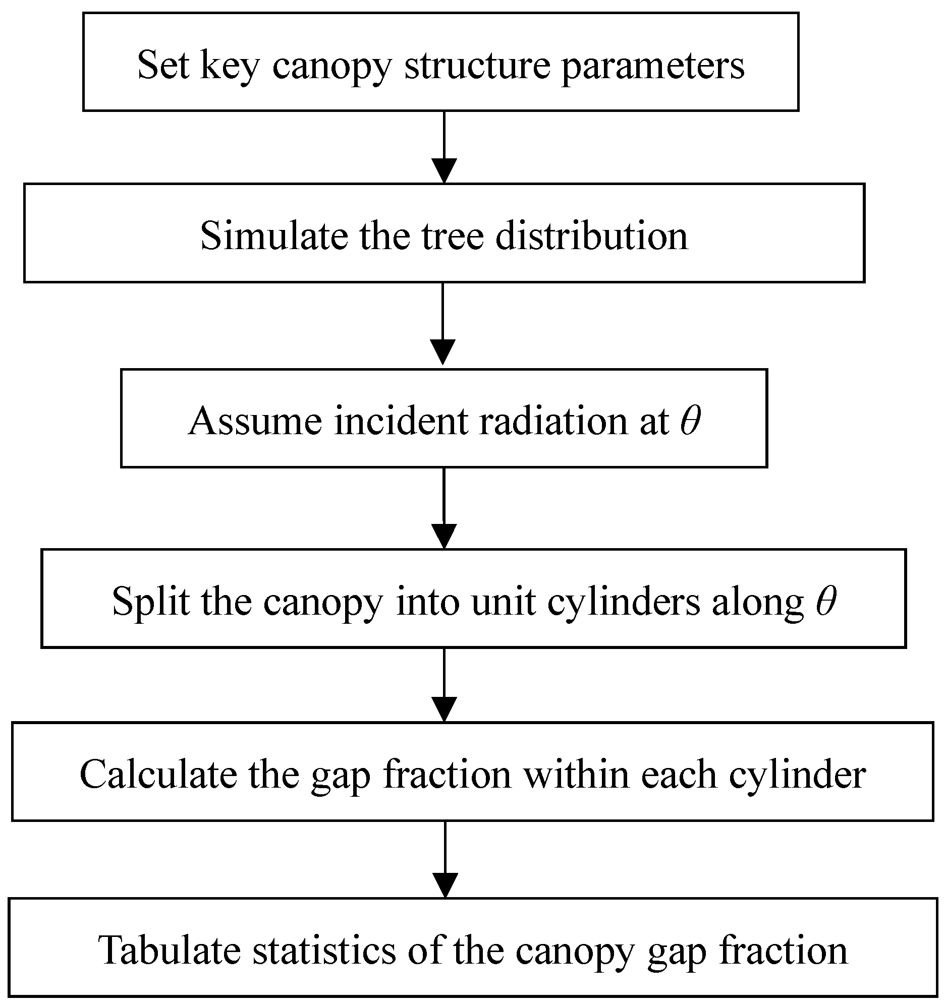
2.2.3. Forest Directional Clumping Index Simulation

The whole forest canopy was segmented into small inclined cylinders along the view direction, while considering the leaf distribution heterogeneity (Figure 3). Average LAI can be calculated for each cylinder according to the tree distribution pattern, i.e., the predefined leaf volume density and cylinder height (related to view zenith angle, θ). Assuming leaves distribute homogeneously within each cylinder, Ω(θ) is 1 for each cylinder at any zenith angle. The cylinder gap fraction $\overline{p_i}$ can be calculated according to Beer’s law as a function of u,

$$\overline{p_i}=\exp \left(-\frac{G_{\theta }}{\cos \theta } u H\right)$$

(15)

where the canopy height is converted to cylinder height through $\cos \theta$, and $G_{\theta }=0.5$. The average gap fraction, $\overline{p(\theta )}$, of the whole canopy can be calculated as the average over all cylinders, and Ω can be obtained from (3).

Key parameters for the simulation include the average LAI of each tree, tree height, crown depth, crown radius, tree density, and parameters defining the tree distribution pattern and research area size.

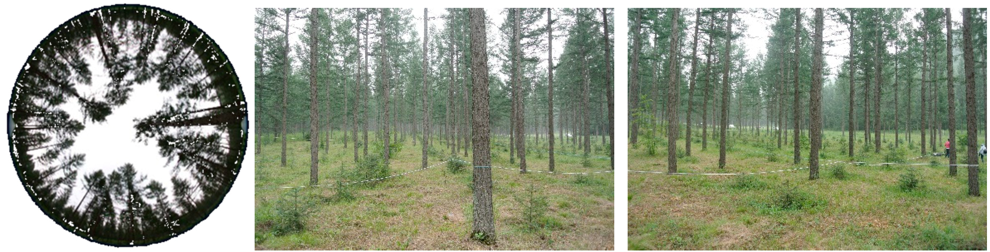
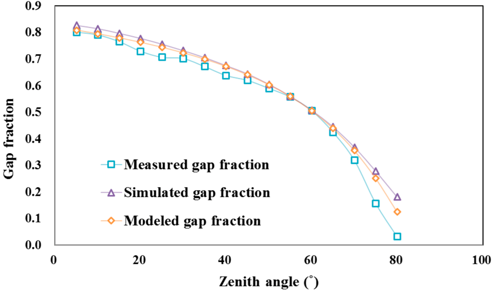
2.3 Forest Ground Measurements

In this paper, two groups of forest Ω(θ) ground measurements were used to validate the analytical model. The ground measurements were collected from published field campaigns and new in situ experiments. Simulation parameters for forest characteristics were set according to practical forest features. The first group of data was obtained from an old Black Spruce (Picea mariana) forest, near Candle Lake, Saskatchewan [8,18] while using TRAC with a measurement error of about 5%.

A second group of measurements was collected at the Saihanba experimental site within Hebei Province in China (117.32°E, 42.40°N). The domain was covered by steppe and forest steppe, with Larch (Larix gmelinii (Rupr.) Rupr.), one of the main tree types.

We measured the Larch gap fraction using hemispherical photographs obtained from a Canon EOS 50D camera with a fish-eye lens, providing orthographic projection and a 180° field of view (Figure 4). The camera setting is introduced in [48]. 53 images were taken within the 45 m × 45 m square. The upward looking hemispherical photograph was further processed using Hemiview 2.1 software (http://www.delta-t.co.uk/product/hemiview/, 5 June 2017) to calculate canopy multiple angle gap fraction. Each hemispherical image was divided into 18 concentric rings between 0° and 90° zenith angle, with a zenith resolution of 5°. The directional gap fraction is calculated for each zenithal ring. The measurement error mainly depends on the threshold setting to discriminate vegetation from sky conditions, which is about 1–3%. Simulation parameters are listed in

Table 2. Forest structure parameters used in the current paper.

Column ID	1	2	3	4	5	6
Height of trunk (m)	0.5	5	0.5	0.5	0, 0.25, …, 1.75	0.5
Crown depth (m)	6.5	1.5	2.28	2.28	2.28	2.07, 2.76, 3.62, 4.38, 5.09, 5.75, 6.37, 6.96
Crown radius (m)	0.45	0.75	0.76	0.76	0.76	0.80, 0.69, 0.60, 0.55, 0.51, 0.48, 0.45, 0.43
H/2R ([-])	7.22	1	1.5	1.5	1.5	1.3, 2, 3, 4, 5, 6, 7, 8
Radius at breast height (m)	0.16	0.15	0.16	0.16	0.16	0.16
${\mathrm{G}}_{\theta }$ ([-])	0.5	0.5	0.5	0.5	0.5	0.5
Average LAI ([-])	4.5	2	0.28, 0.84, 1.40, 1.97, 2.53, 3.09, 3.65, 4.22	2.25	2.25	2.25
Area of research field (ha)	1	5	4	4	4	4
Distribution	Neyman m2 = 4	Poisson	Neyman m2 = 4	Poisson, Neyman m2 = 1, 3, 5, 7, 10, 15, 20	Neyman m2 = 4	Neyman m2 = 4
Tree Number (per ha)	4000	1011	250, 750, …, 3750	2000	2000	2000

, column 2, as collected from the field measurements.

3. Results and Evaluation

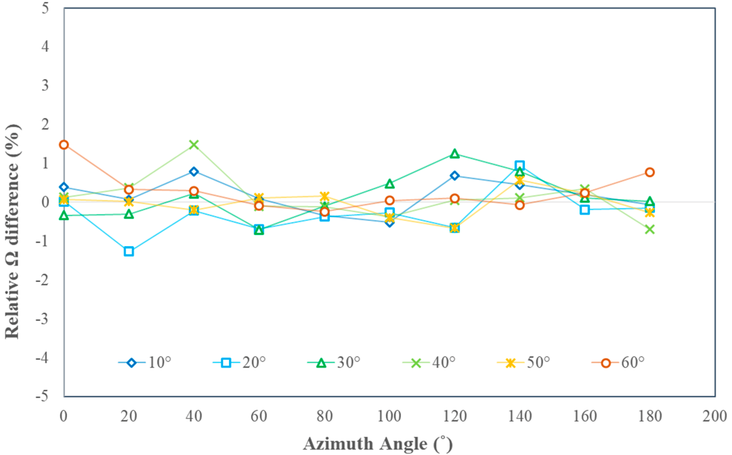
3.1. Crop Directional Clumping Index Validation

The variation of $\mathsf{\Omega }\left(\theta ,\phi \right)$ with View Azimuth Angle ($\phi$) under different $\theta$ is illustrated in Figure 5. The differences between the modeled and simulated results (Figure 6) were randomly distributed with an average of 0, and maximum relative discrepancy <1.5%. The MC simulated and algebraic $\mathsf{\Omega }\left(\theta ,\phi \right)$ are strongly consistent, which provides confidence to analyze crop $\mathsf{\Omega }\left(\theta ,\phi \right)$ variation while using the algebraic model.

The different shapes of $\mathsf{\Omega }\left(\theta ,\phi \right)$ − φ curves reflect the effect of the range angle ${\theta }_c$ of $\mathsf{\Omega }\left(\theta ,\phi \right)$ pattern. When $\phi$ increases from 30° to 90° (perpendicular to the row direction), row period width A decreases, thus ${\theta }_c$ grows; when $\phi$ increases from 90° to 150°, A increases, then ${\theta }_c$ drops. When the $\phi$ is 0° or 180°, i.e., along with the row direction, the gap fraction of row plant is obviously larger than other directions as the row gap always occupies a fraction of the field of view. The $\mathsf{\Omega }\left(\theta ,\phi \right)$ decreases with the growing view zenith angle, which means the crop departures more away from the random status. On the contrary, when the azimuth angle is larger, the $\mathsf{\Omega }\left(\theta ,\phi \right)$ starts growing with view zenith angle and reaches a stable value around one after the view zenith angle higher than the range angle. When the azimuth angle reaches 90°, the ratio of equivalent row width to row height gets its minimum value so that the range angle is smaller than other azimuth directions. These variation trends verify the patterns of crop $\mathsf{\Omega }\left(\theta ,\phi \right)$ in Section 2.1.1 and they show the crop $\mathsf{\Omega }\left(\theta ,\phi \right)$ dispersion at different view angles from constant status.

3.2. Forest Directional Clumping Index Validation

Figure 7 shows the comparison result in the old Black Spruce forest. Since the simulated and measured Ω(θ) were both calculated from the gap fraction, we directly compared the gap fraction for validation. There is high consistency between the measured and simulated gap fraction, validating the proposed simulation method. At zenith angles of >50°, the simulated gap fraction tends to be slightly lower than the measured value due to multiple photon scattering impacting on optical measurements [8,18].

We calculated the gap fraction using Equation (12), with the intra-crown gap pre-processed through simulation as a Look Up Table. The other parameters, including tree density, crown depth, and radius, were set as for previous simulation scenarios. The algebraic method includes the ideal assumption that the trees were Neyman distributed. However, the simulated Poisson distribution may demonstrate higher clustering than ideal situations [49], due to restrictions of the pseudo random number generator in the simulation. One subset of our simulated tree distribution image is demonstrated in Figure 8. Therefore, the calculated gap fraction from the simulation is a little lower than the expected value.

Figure 9 shows the comparison result using the measurements of Larch stand. It shows high consistency between the simulated and measured gap fractions, with small fluctuations at small angles due to random errors and sampling restrictions. When zenith angle of >70°, discrepancies mainly arise due to the hemispherical image being influenced by topography at large angles. Overlapping between trees in the simulation and approximation of the projection area to accumulated discrete square units determine that the average gap fraction in the simulation method is slightly larger than the model in nadir direction, although the number of trees is equal. This difference weakens with increased zenith angle and disappears between 40°–60°, then increases to 0.02 at 80°.

Ω(θ) was indirectly validated through the measured, simulated, and modeled gap fraction, and demonstrated that the model is able to predict the main variation characteristics of Ω(θ).

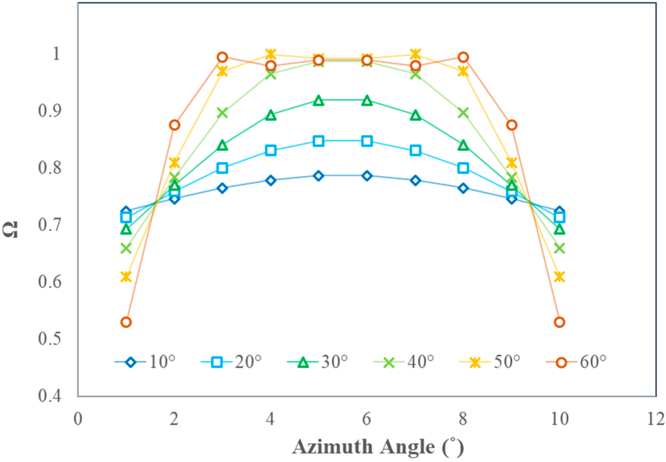
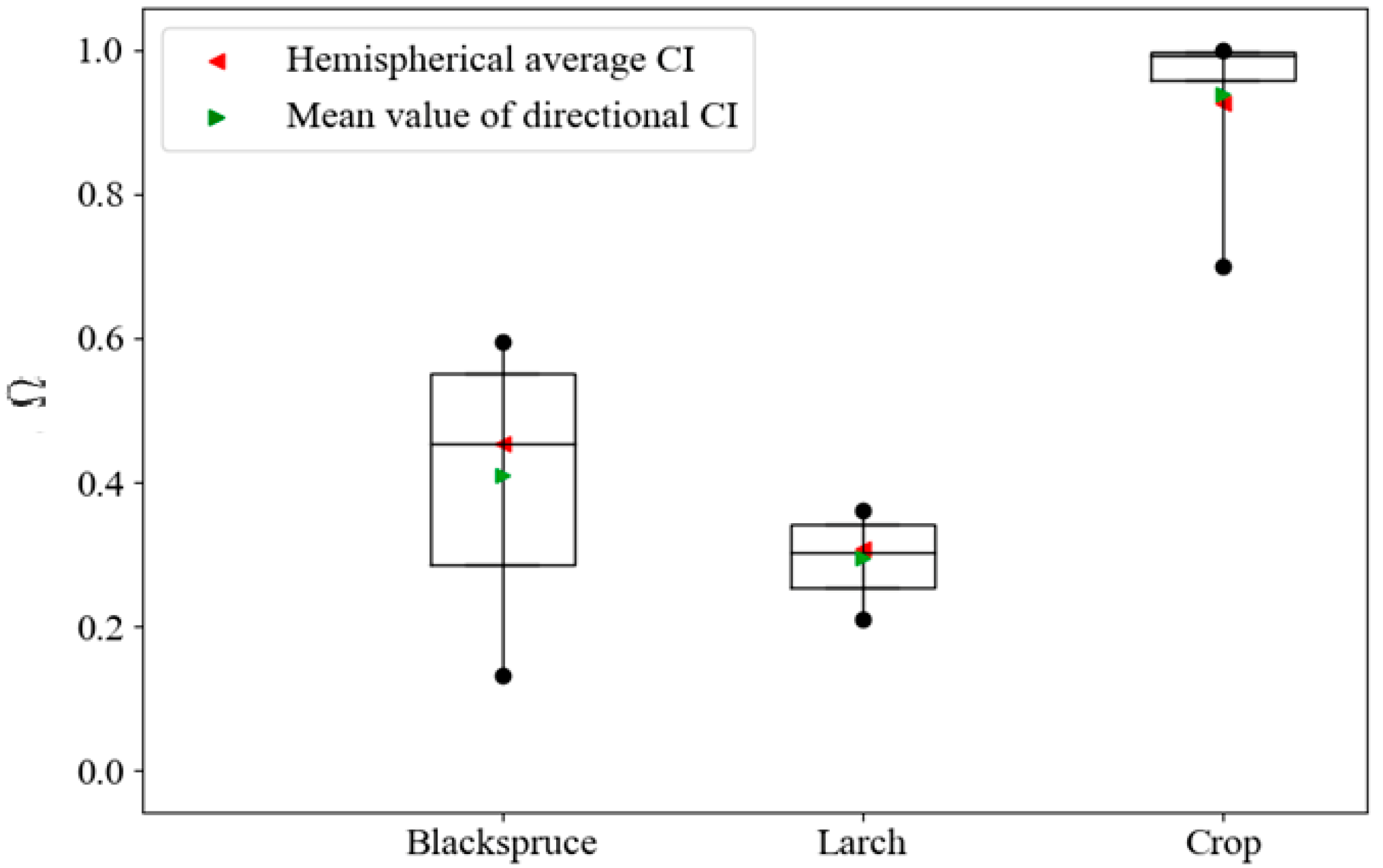
3.3. Assessing the Variation Magnitude of Ω(θ)

Using the proposed models, we assessed the relative variation magnitude of Ω(θ) to indirectly reflect its potential influence on LAI/GPP estimation.

We selected three scenarios, one representing a typical crop example, and the other two matching forest measurements. We first calculated the hemispherical average clumping index ($\tilde{\mathsf{\Omega }}$) for each group by angular integration, where $\tilde{\mathsf{\Omega }}$ represents the commonly used single value of clumping index. The uncertainty due to using $\tilde{\mathsf{\Omega }}$ rather than angle specific Ω(θ) can be assessed from the position of $\tilde{\mathsf{\Omega }}$ in the range of $\mathsf{\Omega }\left(\theta \right)$ (Figure 10). For crop canopies, the discrepancy between $\mathsf{\Omega }\left(\theta \right)$ and $\tilde{\mathsf{\Omega }}$ is more obvious before the zenith angle reaches the range angle. Since the range angle of $\mathsf{\Omega }\left(\theta \right)~\theta$ curve is smaller than 20°, the marker of $\tilde{\mathsf{\Omega }}$ is out of the box. For forest canopies, the angular variation of the black spruce forest is more intense than the larch forest, due to the different Ω(θ) variation range determined by their tree species and growth status. However, all of the variation amplitude relative to $\tilde{\mathsf{\Omega }}$ are large and they should not be neglected.

To further quantify the potential uncertainty caused by ignoring variation of $\mathsf{\Omega }\left(\theta \right)$ with zenith angle, we estimated the relative angular variation magnitude of $\mathsf{\Omega }\left(\theta \right)$ using the index

$$A_V=\frac{{\mathsf{\Omega }}_{max}-{\mathsf{\Omega }}_{min}}{\tilde{\mathsf{\Omega }}}$$

(16)

where A_V values for the example clumping index datasets are listed in

Table 3. Angular clumping index variation statistics.

Canopy Type	Parameters	$\tilde{\mathsf{\Omega }}$	Relative Variation Magnitude Av (%)
Crop	Refer to Figure 2, LAI = 3	0.926	32.4
Black spruce forest	Refer to Table 2, Column 1	0.453	102.3
Larch forest	Refer to Table 2, Column 2	0.308	48.7

. $\mathsf{\Omega }\left(\theta \right)$ variation amplitude for crops can reach 32.4% of its average value. Black spruce has tall and slender crowns, i.e., larger crown shape factor (Section 4.2.4), which leads to larger $\mathsf{\Omega }\left(\theta \right)$ variation range, with Av reaching 102.3%. Larch forest canopy A_V is somewhat lower, mainly due to its relatively smaller $\mathsf{\Omega }\left(\theta \right)$ variation range related to its crown shape factor. This demonstrates that potential uncertainty can arise by ignoring $\mathsf{\Omega }\left(\theta \right)$ variation in practice. Comparing the relative variation magnitude with the allowable error range will help to determine whether or not $\mathsf{\Omega }\left(\theta \right)$ should be treated as constant in practical situations.

Another main application for $\mathsf{\Omega }\left(\theta \right)$ is to estimate the quantity of the terrestrial carbon sink and its dynamic variability. One representative parameter is GPP [33,50]. The proposed method can be used in GPP estimation to explore whether it would improve the accuracy, which would be a fruitful future research direction.

4. Sensitivity Analysis

According to the analytical models, the factors influencing crop Ω(θ) include LAI, leaf foliage distribution, and hedgerow structure, whereas tree density, tree distribution, crown shape, and trunk size influence the forest clumping index. The contribution of these factors are analyzed in this section to assess their relative importance.

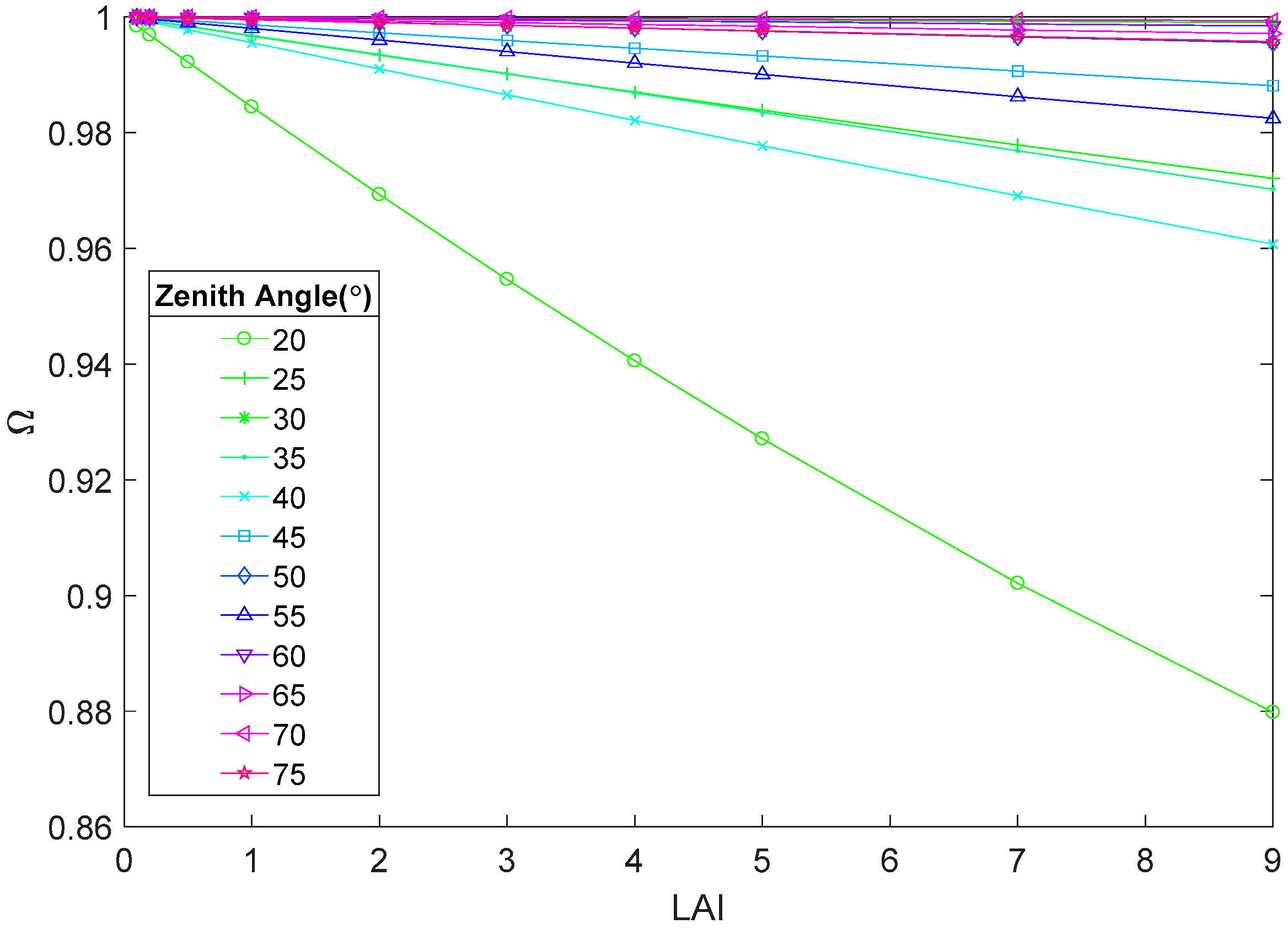
4.1. Factors Influencing Crop Clumping Index Variation

4.1.1. Leaf Area Index

Figure 11 shows that Ω(θ) decreases with increasing LAI in all directions, since heterogeneity is more apparent for larger intra-ridge LAI. Before the zenith angle reaches the range angle, Ω(θ) varies greatly with crop canopy LAI. The view zenith angle of satellite observations is mainly smaller than the range angle, e.g., MODIS view zenith angle is between 0° and 65°. Therefore, Ω(θ) is essential to LAI estimation while using satellite data.

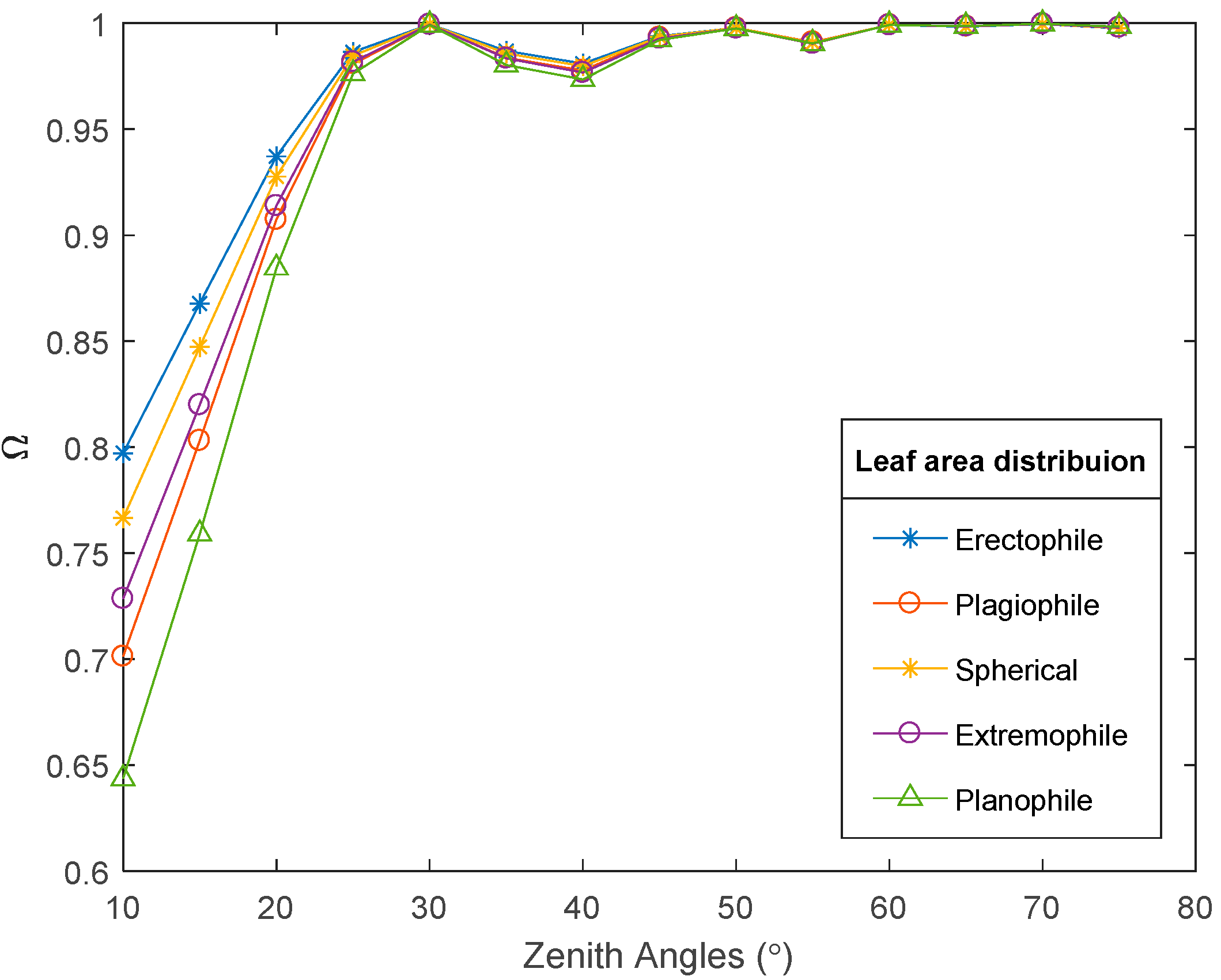
4.1.2. Leaf Angle Distribution

Leaf angle distribution ($G_{\theta }$) is a key parameter influencing Ω(θ) estimation. We estimated crop Ω(θ) for different $G_{\theta }$ functions (Erectophile, Plagiophile, Spherical, Extremophile, and Planophile) (Figure 12) [51]. Figure 13 shows that the effect of different leaf angle distribution is more evident closer to nadir direction. For zenith angle beyond the θ_c, this effect lessens as the crop canopy approaches continuous. Leaf angle distribution and Ω(θ) influence accurate LAI estimation from satellite observations with smaller zenith angles than the range angle.

4.1.3. Row Structure

Row structure is characterized by canopy height, H, and row period width, A. As discussed above, Ω(θ) increases with zenith angle until the range angle, which is controlled by the row structure. Figure 14 shows calculated Ω(θ) for various row structures that are discriminated by A/H, where H = 1, and $a_1/a_2$ = 2:3. Thus, when A/H increases with growing A, the range angle grows, which is consistent with (5).

Generally, the LAI and A/H both have apparent influence on Ω(θ), while $G_{\theta }$ has less influence than the other two factors. However, LAI and A/H are inter-correlative, as we assume that the leaf volume density keeps constant [41], and their influence will partly compensate each other. The influence of all three factors are less obvious at large zenith angles, because Ω(θ) reaches a relatively stable value close to 1 after the zenith angle exceeds the range angle, when the discontinuous crop canopy can be approximately regarded as continuous vegetation canopy.

4.2. Factors Influencing Forest Clumping Index Variation

Crown coverage and crown depth dominates the directional gap fraction and Ω(θ) [21]. In natural cases, crown coverage not only relies on tree density, but also the distribution patterns. Morphological characteristics of tree species also influence the gap fraction. Therefore, we investigated the influence of tree density, tree distribution, crown shape, and trunk size on the clumping index. When we design the simulation experiment and select the parameter values, the following factors were considered. (1) Comparability. The results among different parameters’ results are generally comparable. Some basic setting of the scenarios keeps the same as the ground measured parameters in the black spruce forest; and, (2) Representativeness. For example, we choose an average crown shape of deciduous forest that the crown depth is three times of the crown radius [52]. To avoid the violation to the comparability, the total tree volume was kept constant, so the crown depth was set to 2.28 m and the crown radius was 0.76 m.

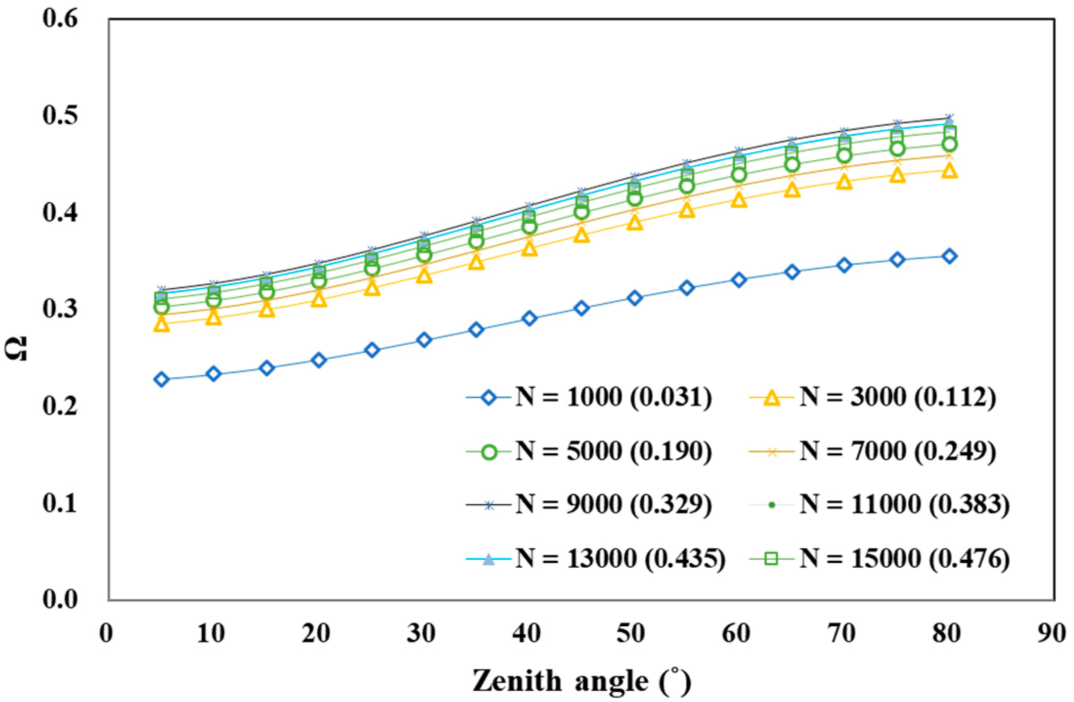
4.2.1. Tree Density

Tree density was varied with individual tree parameters held constant (Table 2, Column 3), and Ω(θ) estimated for each case, as shown in Figure 15. Forest canopy Ω(θ) increases with growing view zenith angle, but since the distribution of vegetation elements is more heterogeneous in forest than crop canopies, Ω(θ) at large zenith angle cannot reach 1, although it also achieves relative stability.

For forests with a given crown coverage (in this simulation, approximately > 0.1), inter-crown gaps disappear rapidly with growing zenith angle, as soil in the field of view is gradually replaced by neighboring trees at the oblique angle. Therefore, Ω(θ) increases for 0–50°. In contrast, for sparse forest, e.g., crown coverage = 0.031 in Figure 15, inter-crown gap dominants the field of view and it cannot be totally counteracted through increasing zenith angle. Thus, Ω(θ) increase for sparse forest is not as apparent as for denser forest and the clumping index generally increases with tree density. An obvious difference can be observed between the N = 1000 line and other lines due to the mutual shadowing and overlapping among crowns. Furthermore, Ω(θ) values for a given zenith angle do not change monotonically with tree density, but they show fluctuations due to changes in the tree arrangement for simulation scenarios, since tree positions were randomly determined. This phenomenon also can be seen in Figure 16, Figure 17 and Figure 18. However, the main trend of Ω(θ) variation remains similar across these factors.

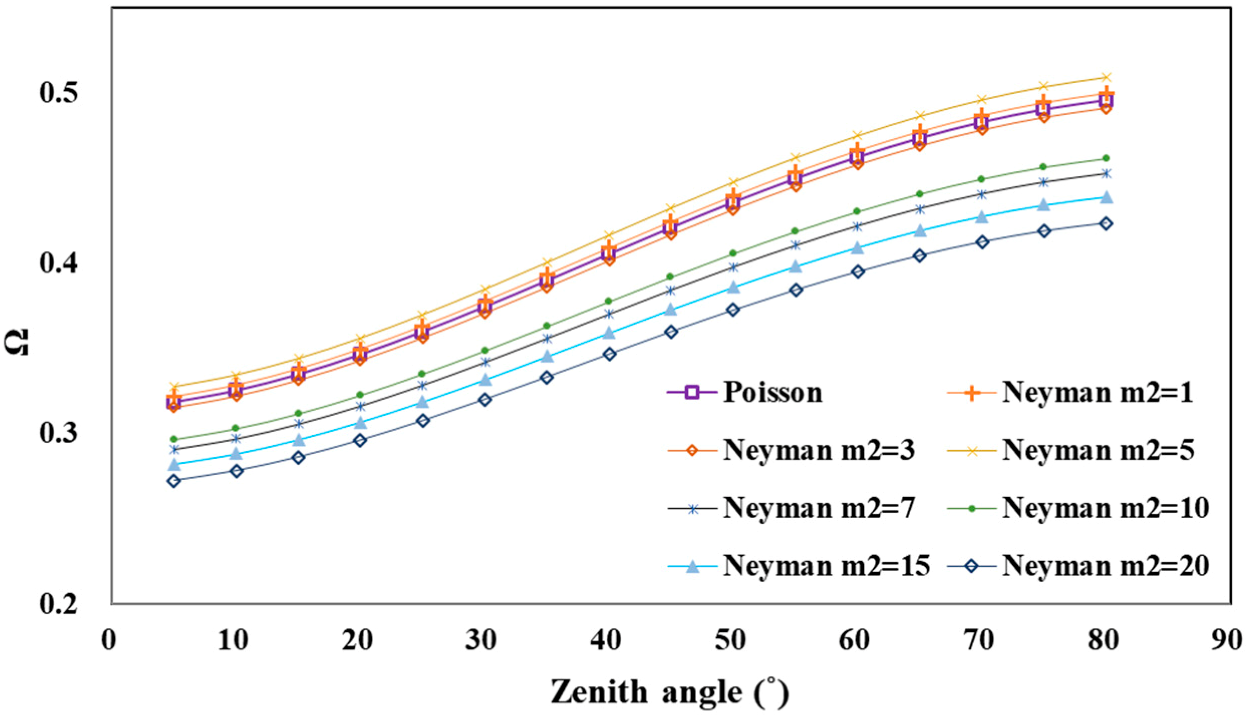
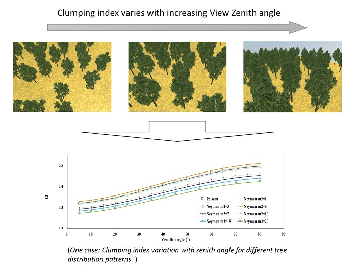
4.2.2. Tree Distribution Pattern

Non-random tree distribution causes clumping and more apparent shadowing among crowns, which also affects canopy Ω(θ) at large zenith angles. Two tree distribution functions were compared: Poisson and Neyman distributions, since these represent random and non-random distributions, respectively [46].

Neyman distribution included m₂ = 1, 2, 5, 10, 20, as shown in Figure 16. When m₂ = 1, the gap fraction distribution is similar to, but not the same as, the Poisson distribution. As m₂ increases, the clumping effect between trees and intra-crown gap fraction increase. However, this combined effect on Ω(θ) is not large. When m₂ ≤ 5, Ω(θ) difference between sample lines <0.02. This demonstrates that the slight non-random distributions in natural forests has little influence on canopy level Ω(θ). But, if the non-random distribution is dominant, its influence on Ω(θ) cannot be ignored. For example, the Ω(θ) difference between the sample line with m₂ = 5 and that with m₂ = 20 can reach 0.08 at large zenith angles.

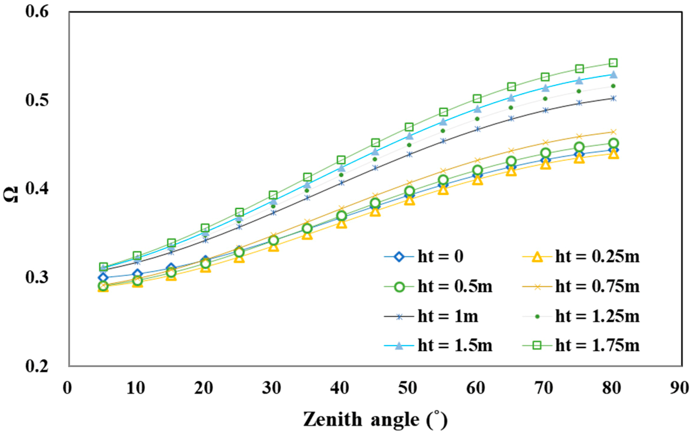
4.2.3. Trunk Height

The proposed algebraic models for forest clumping index estimation parameterized tree trunk influence. The influence of tree trunk on gap fraction would be great for high trunk tree species, such as the black spruce forest that is considered above.

Figure 17 shows that the influence of trunk is more important at higher zenith angles, because the fraction of visible trunk grows with zenith angle from only the cross section at nadir direction. Higher trunk fraction in the field of view leads to lower gap fraction, causing increased Ω(θ) for constant average LAI. The variation magnitude depends on the forest scenario, which is larger than 0.1 in this example and it should not be neglected.

Note that increased trunk size would increase the equivalent average LAI, since the trunk is one of the vegetation elements, but the average LAI was set as constant in the simulation (Figure 17) to realize monofactor sensitivity analysis and highlight trunk height influence on directional Ω(θ).

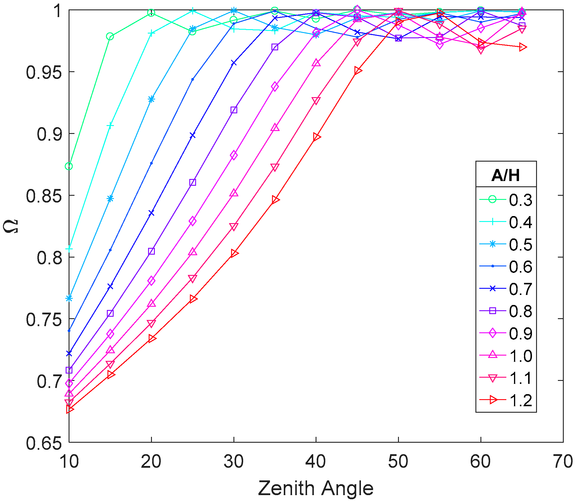
4.2.4. Crown Shape

The tree crown was simplified as an ellipsoid in the proposed model. One convenience of this approach is that different species can be discriminated through the crown shape factor $h/2R$ combined with horizontal radius, R.

To highlight crown shape influence on canopy Ω(θ), we kept the crown column constant while changing the crown shape factor (Figure 18). Table 2 shows that crown depth, radius, and their ratio change synchronously.

As the ratio between crown depth and radius increases, there is more obvious increasing Ω(θ) trend with zenith angle. When $h/2R=2$, i.e., the crown is spherical, there is only slight Ω(θ) increase with increasing zenith angle (~0.2 in this example). However, when $h/2R=8$, implying that a deep canopy, Ω(θ) increased with growing zenith angle, and approaches 1.

At near nadir direction, lower crown depth and radius ratios correspond to larger horizontal projection for each crown when the column is fixed. This larger projection corresponds to lower gap fraction and results in larger Ω(θ). However, curves with higher crown depth and radius ratios demonstrate Ω(θ) increase with growing zenith angle, because neighboring crowns connect together earlier as the zenith angle increases.

Thus, the forest is more similar to a continuous canopy at larger zenith angles. This continuous effect is more apparent for larger crown depth and radius ratios, and it occurs earlier in the solar zenith dimension.

5. Conclusions

This study investigated the directional clumping effects from typical discontinuous vegetation canopies, including crop and forest. The results verified that the angular variation of the clumping index not only exists, but also reaches notable magnitude for practical cases.

We proposed analytical models to predict the $\mathsf{\Omega }\left(\theta \right)$ of crop and forest using structural parameters. The models were validated using simulations for near real cases, and also compared with several sets of ground measurements collected from field experiments and literature. The comparisons provide confidence that the calculated and simulated gap fractions fit ground measurements well.

The analytical model derived from the definition shows that crop $\mathsf{\Omega }\left(\theta \right)$ is mainly determined by the row structures, LAI and leaf angle distribution. The effect of these parameters on $\mathsf{\Omega }\left(\theta \right)$ will decrease at large view zenith angles. In contrast, forest $\mathsf{\Omega }\left(\theta \right)$ is dominated by tree density, tree distribution pattern, crown shape, and trunk size. Their influence on the variation magnitude of $\mathsf{\Omega }\left(\theta \right)$ are all not negligible.

Is it necessary to introduce $\mathsf{\Omega }\left(\theta \right)$? In most practical applications of vegetation remote sensing, average clumping index $\tilde{\mathsf{\Omega }}$ has played the leading role and provided the bridge from effective LAI to actual LAI. Since $\mathsf{\Omega }$ has integrated the overall hemispherical influence, it could be conveniently rendered as a unified global map. However, the large $\mathsf{\Omega }\left(\theta \right)$ variation in the angular dimension and the influence of clumping index on LAI and GPP prompt us to study $\mathsf{\Omega }\left(\theta \right)$ systematically. We intend to investigate the proposed approach to further assess the difference between LAI and GPP products that are derived using $\tilde{\mathsf{\Omega }}$ or $\mathsf{\Omega }\left(\theta \right)$, and validate the results using abundant ground measurements. This expansion will be useful to judge whether $\mathsf{\Omega }\left(\theta \right)$ should be introduced for standard LAI and GPP production. Another potential option is to apply $\mathsf{\Omega }\left(\theta \right)$, as the reference to select an optimal average $\tilde{\mathsf{\Omega }}$.

The current research still suffers from many problems and limitations.

(1)

The crop model was developed for row structure with homogenous plant elements within the hedgerow. It is not suited for other structures or intercropping of multiple crops. The forest model has not considered the complementary tree species. The tree distribution pattern, LAI, and gap fraction will be quite different in a scenario with the mixture of complementary trees [53].

(2)

The influence of the crown shape model needs further investigation. Currently, we have assumed the tree crown as vertical ellipsoid. For most species, the crowns can quite well be represented by ellipsoids; however, some exceptions, such as the boreal needle forest, can be fit better by cones McPherson [54] stated that the mean difference between the crown volume measures from the assumptions of crown shape as paraboloids, vertical ellipsoids, and horizontal ellipsoids are 10%. In tropical forest, the multi-stem trees are very common. The current crown shape model might be not valid for them. The further effect of crown shape model on the clumping index needs to be discussed for different species.

(3)

Further comprehensive sensitivity analysis is expected. The analysis in this paper is restricted to be a mono parameter analysis and the variation range of all the parameters is independent. This is only the first step to observe the influence of each single parameter under specific conditions. In the natural environment, there is a size-density allometry of plants under self-thinning as the resources for growing are limited. The crown projection area scales to stem diameter [53]. Besides, LAI and LAD many vary simultaneously. Therefore, a multiple simultaneous analysis is needed to avoid the risk to misconstrue simple size effects as changes in the crown morphology.

Further research is required to refine this analysis. The analytical directional clumping index models would be applied in the unified model of bidirectional reflectance distribution function for the vegetation canopy [40]. With the Unified BRDF model, the leaf area index can be analytically estimated. Then, further validation using ground measurements and inter-comparison with other products will demonstrate whether or how much the introduction of directional clumping index would improve the LAI accuracy.

References

- Chen, J.M.; Liu, J.; Leblanc, S.G.; Lacaze, R.; Roujean, J. Multi-angular optical remote sensing for assessing vegetation structure and carbon absorption. Remote Sens. Environ. 2003, 84, 516–525. [Google Scholar] [CrossRef] [Green Version]
- Duthoit, S.; Demarez, V.; Gastellu-Etchegorry, J.; Martin, E.; Roujean, J. Assessing the effects of the clumping phenomenon on BRDF of a maize crop based on 3D numerical scenes using DART model. Agric. For. Meteorol. 2008, 148, 1341–1352. [Google Scholar] [CrossRef]
- Qin, Z.; Li, Z.; Cheng, F.; Chen, J.; Liang, B. Influence of canopy structural characteristics on cooling and humidifying effects of Populus tomentosa community on calm sunny summer days. Landsc. Urban Plan. 2014, 127, 75–82. [Google Scholar] [CrossRef]
- Chen, J.M.; Menges, C.H.; Leblanc, S.G. Global mapping of foliage clumping index using multi-angular satellite data. Remote Sens. Environ. 2005, 97, 447–457. [Google Scholar] [CrossRef]
- Jonckheere, I.; Fleck, S.; Nackaerts, K.; Muys, B.; Coppin, P.; Weiss, M.; Baret, F. Review of methods for in situ leaf area index determination: Part I. Theories, sensors and hemispherical photography. Agric. For. Meteorol. 2004, 121, 19–35. [Google Scholar] [CrossRef]
- Fassnacht, K.S.; Gower, S.T.; Norman, J.M.; McMurtric, R.E. A comparison of optical and direct methods for estimating foliage surface area index in forests. Agric. For. Meteorol. 1994, 71, 183–207. [Google Scholar] [CrossRef]
- Nilson, T. Inversion of gap frequency data in forest stands. Agric. For. Meteorol. 1999, 98–99, 437–448. [Google Scholar] [CrossRef]
- Chen, J.M.; Leblanc, S.G. A four-scale bidirectional reflectance model based on canopy architecture. IEEE Trans. Geosci. Remote Sens. 1997, 35, 1316–1337. [Google Scholar] [CrossRef] [Green Version]
- Pisek, J.; Chen, J.M.; Lacaze, R.; Sonnentag, O.; Alikas, K. Expanding global mapping of the foliage clumping index with multi-angular POLDER three measurements: Evaluation and topographic compensation. ISPRS J. Photogramm. Remote Sens. 2010, 65, 341–346. [Google Scholar] [CrossRef]
- Miller, J.B. A formula for average foliage density. Aust. J. Bot. 1967, 15, 141–144. [Google Scholar] [CrossRef]
- Watson, D.J. Comparative physiological studies on the growth of field crops: I. Variation in net assimilation rate and leaf area between species and varieties, and within and between years. Ann. Bot. 1947, 11, 41–76. [Google Scholar] [CrossRef]
- Chen, J.M.; Black, T.A. Defining leaf area index for non-flat leaves. Plant Cell Environ. 1992, 15, 421–429. [Google Scholar] [CrossRef]
- Zheng, G.; Moskal, L.M. Retrieving leaf area index (LAI) using remote sensing: Theories, methods and sensors. Sensors 2009, 9, 2719–2745. [Google Scholar] [CrossRef] [PubMed]
- Weiss, M.; Baret, F.; Smith, G.J.; Jonckheere, I.; Coppin, P. Review of methods for in situ leaf area index (LAI) determination: Part II. Estimation of LAI, errors and sampling. Agric. For. Meteorol. 2004, 121, 37–53. [Google Scholar] [CrossRef]
- Bréda, N.J. Ground-based measurements of leaf area index: A review of methods, instruments and current controversies. J. Exp. Bot. 2003, 54, 2403–2417. [Google Scholar] [CrossRef] [PubMed]
- Kucharik, C.J.; Norman, J.M.; Murdock, L.M.; Gower, S.T. Characterizing canopy nonrandomness with a multiband vegetation imager (MVI). J. Geophys. Res. Atmos. (1984–2012) 1997, 102, 29455–29473. [Google Scholar] [CrossRef] [Green Version]
- Norman, J.M.; Jarvis, P.G. Photosynthesis in Sitka spruce (Picea sitchensis (Bong.) Carr.). III. Measurements of canopy structure and interception of radiation. J. Appl. Ecol. 1974, 11, 375–398. [Google Scholar] [CrossRef]
- Chen, J.M. Optically-based methods for measuring seasonal variation of leaf area index in boreal conifer stands. Agric. For. Meteorol. 1996, 80, 135–163. [Google Scholar] [CrossRef]
- Ryu, Y.; Nilson, T.; Kobayashi, H.; Sonnentag, O.; Law, B.E.; Baldocchi, D.D. On the correct estimation of effective leaf area index: Does it reveal information on clumping effects? Agric. For. Meteorol. 2010, 150, 463–472. [Google Scholar] [CrossRef]
- Sinoquet, H.; Sonohat, G.; Phattaralerphong, J.; Godin, C. Foliage randomness and light interception in 3-D digitized trees: An analysis from multiscale discretization of the canopy. Plant Cell Environ. 2005, 28, 1158–1170. [Google Scholar] [CrossRef]
- Kucharik, C.J.; Norman, J.M.; Gower, S.T. Characterization of radiation regimes in nonrandom forest canopies: Theory, measurements, and a simplified modeling approach. Tree Physiol. 1999, 19, 695–706. [Google Scholar] [CrossRef] [PubMed]
- Kuusk, A. A fast, invertible canopy reflectance model. Remote Sens. Environ. 1995, 51, 342–350. [Google Scholar] [CrossRef]
- Leblanc, S.G.; Chen, J.M. A practical scheme for correcting multiple scattering effects on optical LAI measurements. Agric. For. Meteorol. 2001, 110, 125–139. [Google Scholar] [CrossRef] [Green Version]
- Gonsamo, A.; Pellikka, P. The computation of foliage clumping index using hemispherical photography. Agric. For. Meteorol. 2009, 149, 1781–1787. [Google Scholar] [CrossRef]
- Wang, Y.; Woodcock, C.E.; Buermann, W.; Stenberg, P.; Voipio, P.; Smolander, H.; Häme, T.; Tian, Y.; Hu, J.; Knyazikhin, Y.; et al. Evaluation of the MODIS LAI algorithm at a coniferous forest site in Finland. Remote Sens. Environ. 2004, 91, 114–127. [Google Scholar] [CrossRef]
- He, L.; Chen, J.M.; Pisek, J.; Schaaf, C.B.; Strahler, A.H. Global clumping index map derived from the MODIS BRDF product. Remote Sens. Environ. 2012, 119, 118–130. [Google Scholar] [CrossRef]
- Pisek, J.; Ryu, Y.; Sprintsin, M.; He, L.; Oliphant, A.J.; Korhonen, L.; Kuusk, J.; Kuusk, A.; Bergstrom, R.; Verrelst, J.; et al. Retrieving vegetation clumping index from Multi-angle Imaging SpectroRadiometer (MISR) data at 275m resolution. Remote Sens. Environ. 2013, 138, 126–133. [Google Scholar] [CrossRef]
- Graefe, J.; Sandmann, M. Shortwave radiation transfer through a plant canopy covered by single and double layers of plastic. Agric. For. Meteorol. 2015, 201, 196–208. [Google Scholar] [CrossRef]
- Rautiainen, M.; Stenberg, P. On the angular dependency of canopy gap fractions in pine, spruce and birch stands. Agric. For. Meteorol. 2015, 206, 1–3. [Google Scholar] [CrossRef]
- Stenberg, P.; Manninen, T. The effect of clumping on canopy scattering and its directional properties: A model simulation using spectral invariants. Int. J. Remote Sens. 2015, 36, 5178–5191. [Google Scholar] [CrossRef]
- Garrigues, S.; Shabanov, N.V.; Swanson, K.; Morisette, J.T.; Baret, F.; Myneni, R.B. Intercomparison and sensitivity analysis of Leaf Area Index retrievals from LAI-2000, AccuPAR, and digital hemispherical photography over croplands. Agric. For. Meteorol. 2008, 148, 1193–1209. [Google Scholar] [CrossRef] [Green Version]
- Piayda, A.; Dubbert, M.; Werner, C.; Correia, A.V.; Pereira, J.S.; Cuntz, M. Influence of woody tissue and leaf clumping on vertically resolved leaf area index and angular gap probability estimates. For. Ecol. Manag. 2015, 340, 103–113. [Google Scholar] [CrossRef]
- Chen, J.M.; Mo, G.; Pisek, J.; Liu, J.; Deng, F.; Ishizawa, M.; Chan, D. Effects of foliage clumping on the estimation of global terrestrial gross primary productivity. Glob. Biogeochem. Cycles 2012, 26. [Google Scholar] [CrossRef] [Green Version]
- Leblanc, S.G.; Fernandes, R.; Chen, J.M. Recent advancements in optical field leaf area index, foliage heterogeneity, and foliage angular distribution measurements. In Proceedings of the 2002 IEEE International Geoscience and Remote Sensing Symposium (IGARSS’02), Toronto, ON, Canada, 24–28 June 2002; pp. 2902–2904. [Google Scholar]
- Saitoh, T.M.; Nagai, S.; Noda, H.M.; Muraoka, H.; Nasahara, K.N. Examination of the extinction coefficient in the Beer-Lambert law for an accurate estimation of the forest canopy leaf area index. For. Sci. Technol. 2012, 8, 67–76. [Google Scholar] [CrossRef]
- Andrieu, B.; Sinoquet, H. Evaluation of structure description requirements for predicting gap fraction of vegetation canopies. Agric. For. Meteorol. 1993, 65, 207–227. [Google Scholar] [CrossRef]
- Fan, W.; Yan, B.; Xu, X. Crop area and leaf area index simultaneous retrieval based on spatial scaling transformation. Sci. China Earth Sci. 2010, 53, 1709–1716. [Google Scholar] [CrossRef]
- Peng, J.; Fan, W.; Xu, X.; Wang, L.; Liu, Q.; Li, J.; Zhao, P. Estimating Crop Albedo in the Application of a Physical Model Based on the Law of Energy Conservation and Spectral Invariants. Remote Sens. 2015, 7, 15536–15560. [Google Scholar] [CrossRef] [Green Version]
- Li, X.; Strahler, A.H. Geometric-optical bidirectional reflectance modeling of a conifer forest canopy. IEEE Trans. Geosci. Remote 1986, 6, 906–919. [Google Scholar] [CrossRef]
- Xu, X.; Fan, W.; Li, J.; Zhao, P.; Chen, G. A unified model of bidirectional reflectance distribution function for the vegetation canopy. Sci. China Earth Sci. 2017, 60, 463–477. [Google Scholar] [CrossRef]
- Yan, B.; Xu, X.; Fan, W. A unified canopy bidirectional reflectance (BRDF) model for row ceops. Sci. China Earth Sci. 2012, 55, 824–836. [Google Scholar] [CrossRef]
- Nilson, T. A theoretical analysis of the frequency of gaps in plant stands. Agric. Meteorol. 1971, 8, 25–38. [Google Scholar] [CrossRef]
- Chen, J.M.; Cihlar, J. Retrieving leaf area index of boreal conifer forests using Landsat TM images. Remote Sens. Environ. 1996, 55, 153–162. [Google Scholar] [CrossRef]
- Nguyen, H.H.; Uria Diez, J.; Wiegand, K. Spatial distribution and association patterns in a tropical evergreen broad-leaved forest of north-central Vietnam. J. Veg. Sci. 2015, 27, 318–327. [Google Scholar] [CrossRef]
- Nilson, T.; Peterson, U. A forest canopy reflectance model and a test case. Remote Sens. Environ. 1991, 37, 131–142. [Google Scholar] [CrossRef]
- Franklin, J.; Michaelsen, J.; Strahler, A.H. Spatial analysis of density dependent pattern in coniferous forest stands. Vegetatio 1985, 64, 29–36. [Google Scholar] [CrossRef]
- Neyman, J. On a new class of “contagious” distributions, applicable in entomology and bacteriology. Ann. Math. Stat. 1939, 10, 35–57. [Google Scholar] [CrossRef]
- Li, J.; Fan, W.; Liu, Y.; Zhu, G.; Peng, J.; Xu, X. Estimating Savanna Clumping Index Using Hemispherical Photographs Integrated with High Resolution Remote Sensing Images. Remote Sens. 2016, 9, 52. [Google Scholar] [CrossRef]
- Chen, J.M.; Cihlar, J. Plant canopy gap-size analysis theory for improving optical measurements of leaf-area index. Appl. Opt. 1995, 34, 6211–6222. [Google Scholar] [CrossRef] [PubMed]
- Kotchenova, S.Y.; Song, X.; Shabanov, N.V.; Potter, C.S.; Knyazikhin, Y.; Myneni, R.B. Lidar remote sensing for modeling gross primary production of deciduous forests. Remote Sens. Environ. 2004, 92, 158–172. [Google Scholar] [CrossRef]
- Ross, J.K. The Radiation Regime and the Architecture of Plant Stands; Junk W. In Pubs: The Hague, The Netherlands, 1981. [Google Scholar]
- Popescu, S.C.; Zhao, K. A voxel-based lidar method for estimating crown base height for deciduous and pine trees. Remote Sens. Environ. 2008, 112, 767–781. [Google Scholar] [CrossRef]
- Pretzsch, H. Canopy space filling and tree crown morphology in mixed-species stands compared with monocultures. For. Ecol. Manag. 2014, 327, 251–264. [Google Scholar] [CrossRef]
- McPherson, E.G.; Rowntree, R.A. Geometric solids for simulation of tree crowns. Landsc. Urban Plan. 1988, 15, 79–83. [Google Scholar] [CrossRef]