Flood Hazard Assessment Supported by Reduced Cost Aerial Precision Photogrammetry

Abstract

Increasing flood hazards worldwide due to the intensification of hydrological events and the development of adaptation-mitigation strategies are key challenges that society must address. To minimize flood damages, one of the crucial factors is the identification of flood prone areas through fluvial hydraulic modelling in which a detailed knowledge of the terrain plays an important role for reliable results. Recent studies have demonstrated the suitability of the Reduced Cost Aerial Precision Photogrammetry (RC-APP) technique for fluvial applications by accurate-detailed-reliable Digital Terrain Models (DTMs, up to: ≈100 point/m²; vertical-uncertainty: ±0.06 m). This work aims to provide an optimal relationship between point densities and vertical-uncertainties to generate more reliable fluvial hazard maps by fluvial-DTMs. This is performed through hydraulic models supported by geometric models that are obtained from a joint strategy based on Structure from Motion and Cloth Simulation Filtering algorithms. Furthermore, to evaluate vertical-DTM, uncertainty is proposed as an alternative approach based on the method of robust estimators. This offers an error dispersion value analogous to the concept of standard deviation of a Gaussian distribution without requiring normality tests. This paper reinforces the suitability of new geomatic solutions as a reliable-competitive source of accurate DTMs at the service of a flood hazard assessment.

1. Introduction

Floods are probably the most hazardous natural event worldwide as well as the main cause of numerous human being losses and severe economic damages [1,2,3]. From the years 2000 to 2012, the European Union experienced an average annual damage due to floods of €4.2 billion, which could be increased up to €23.5 billion by 2050 [4]. In particular, 2013 flood events in central Europe had an estimated cost of €12 billion [5] and, in Spain, floods are the natural hazard that causes the greatest social and economic losses [6] with estimated annual costs of €0.87 billion predicted to occur from 2004 to 2033 [7]. Moreover, the intensification of hydrological phenomena (rainfall, flood and drought, mainly) is a tangible reality even by non-experts with more frequent magnitudes and more unpredictable extreme events [8,9,10,11,12,13,14]. Recent studies have already shown a direct relationship among the intensification of hydrological events and climate change [15,16,17,18]. This, combined with population growth in flood prone areas, is increasing the flood damages [19,20,21,22,23].

Under such circumstances, reducing the flood hazard must be an absolute necessity. This global challenge is leading society to take protective measures [21,24,25,26], which is mainly based on the analysis of the three components inherent to a natural hazard: (i) occurrence probability, (ii) level exposure, and (iii) vulnerability hazards [2,5,27]. Traditionally, the scientific community had focused its efforts on risk occurrence probability. However, recently, the focus is shifting to risk consequences [2], its mitigation [28], and damage reductions [24], which is also as a consequence to the growing variability of the hydrological variables [12,13].

To assess a flood hazard, it is widely accepted to analyze the conceptual scheme into three steps, which are exposed in de Moel et al. [29]. The three steps are: (i) to estimate discharge flows for particular return periods from frequency analyses on discharge records, adjusted to extreme value distributions or specific rainfall-runoff models, (ii) to translate discharge flows into water levels by rating (stage-discharge) curves or 1D or 2D hydrodynamic models, and (iii) calculate the inundated area supported by Digital Terrain Models (DTMs). Nevertheless, this seemingly simple scheme hides a complex and non-trivial three-dimensional hydrodynamic process [11,30] full of uncertainties [30,31].

Flood modeling involves multiple key aspects including: (i) hydrological model or flood wave characteristics [29], (ii) fluvial geomorphology issues [32,33,34], (iii) the influence of infrastructures such as bridges, dams, or buildings [22,35,36], (iv) structure of hydraulic model, its equations, methods to solve them, and simplifications applied to the model [11,23,37], (v) flow propagation methods [3,38], (vi) human-induced changes in land use [21], (vii) the roughness coefficient [11,31], (viii) vulnerability/damage curves of the potential effects of the flow [22,39,40], and (viii) topographic data of flood prone areas [3,33,41,42,43].

This multidisciplinary nature makes flood hazard assessment an active research line in the scientific community. For example, Huang and Qin [31] determine that the Manning’s roughness coefficient (Manning’s n) notably affect flood inundation predictions. For their part, Milanesi et al. [22] argue that the flood assessment must be based on an appropriate combination of flow depth and velocity by using duly designed vulnerability curves. Macchione et al. [3] shows as key factors the mathematical model and numerical schemes applied to flow propagation in addition to the terrain model and the existing constructions. In Arrighi et al. [39], the flood depth, velocity, flood duration, and the uncertainty in depth–damage curves are shown as relevant issues versus uncertainties in hydrological-hydraulic models and land uses. Falcao et al. [44] and Md Ali et al. [45] investigate the influence of elevation modeling on hydrodynamic modeling results and both determined that DTMs are one the most fundamental inputs for reliable flood modeling. All these studies and their conclusions reinforce, a fortiori, the multidisciplinary and integrated nature of a flood hazard assessment.

According to Schanze et al. [46], for reducing natural flood hazards, only two different actions may be applied through: (i) “structural” measures based on works of hydraulic engineering, which modify hydrological-hydraulic characteristics of floods, and (ii) all other interventions called “non-structural”. These latter are especially interesting in this research because: (i) they modify the susceptibility of the inundated area without acting on the flood flow itself [23,46,47], (ii) they are essentially focused on potential consequences [47], and (iii) they are an accessible way to reduce the flood hazard [48]. In this sense, the most important non-structural measure is floodplain planning [40] whose goal is to properly identify flood prone areas. Thus, it is possible to define constraints of land uses on the floodplain and reduce the flood hazard [24,49]. Essentially, this involves the interplay between flow, the physical environment, and society [7,50].

On the other hand, recent geomatic advances on: (a) instruments and techniques for data acquisition, (b) imagery processing algorithms, and (c) alternative aerial platforms have led the appearance of effective (time-cost) solutions in response to the growing need of suitable topographic data for flood modeling [41]. In this sense, a Reduced Cost Aerial Precision Photogrammetry methodology (RC-APP, [43]) is one of them based on Digital Photogrammetry (DP).

While topographic data sources traditionally applied to 3D ground modeling such as Global Navigation Satellite System, Airborne/Terrestrial Laser Scanning and Satellite images have been extensively discussed in many prior studies [45,51,52,53,54,55,56]. The influence of spatial resolution and vertical uncertainty on flood modeling and hazard assessment have received far less attention. This study aims to provide an optimal relationship between the point densities and vertical-uncertainties to generate more reliable fluvial hazard maps.

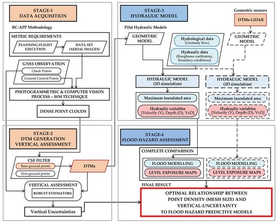
This paper forms part of the research line exposed in Zazo et al. [42,43] and Zazo [57] that is characterized by hybridizing geomatics and fluvial hydraulics with the purpose of improving the knowledge of flood behavior. In this case, an accurate-high density point cloud was obtained through RC-APP methodology. Next, point clouds with different point densities were generated. Then, to reduce the vegetation influence on DTMs, a novel point cloud filter named Cloth Simulation Filtering (CSF; [58]) was applied to classify point clouds into ground/non-ground. After that, different bare-ground DTMs were generated and their vertical-uncertainties were also assessed. Subsequently, 2D hydraulic models were performed, which were supported by previous DTMs. The results achieved (flood modeling and hazard assessment) were analyzed in-depth. Lastly, to reveal the potential that the approach based on RC-APP and CSF have on flood hazard assessment, the results were compared with those obtained through the Light Detection and Ranging data (LiDAR) technique.

In addition, this work proposes a variant of the non-parametric Robust Estimators (RE) method [42] for assessing the vertical-DTM uncertainty. This provides a dispersion value of error comparable to the concept of standard deviation from a Gaussian distribution without requiring normality tests.

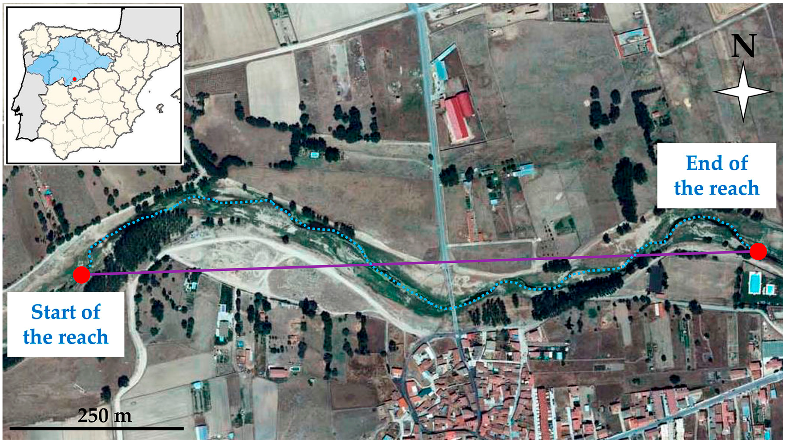
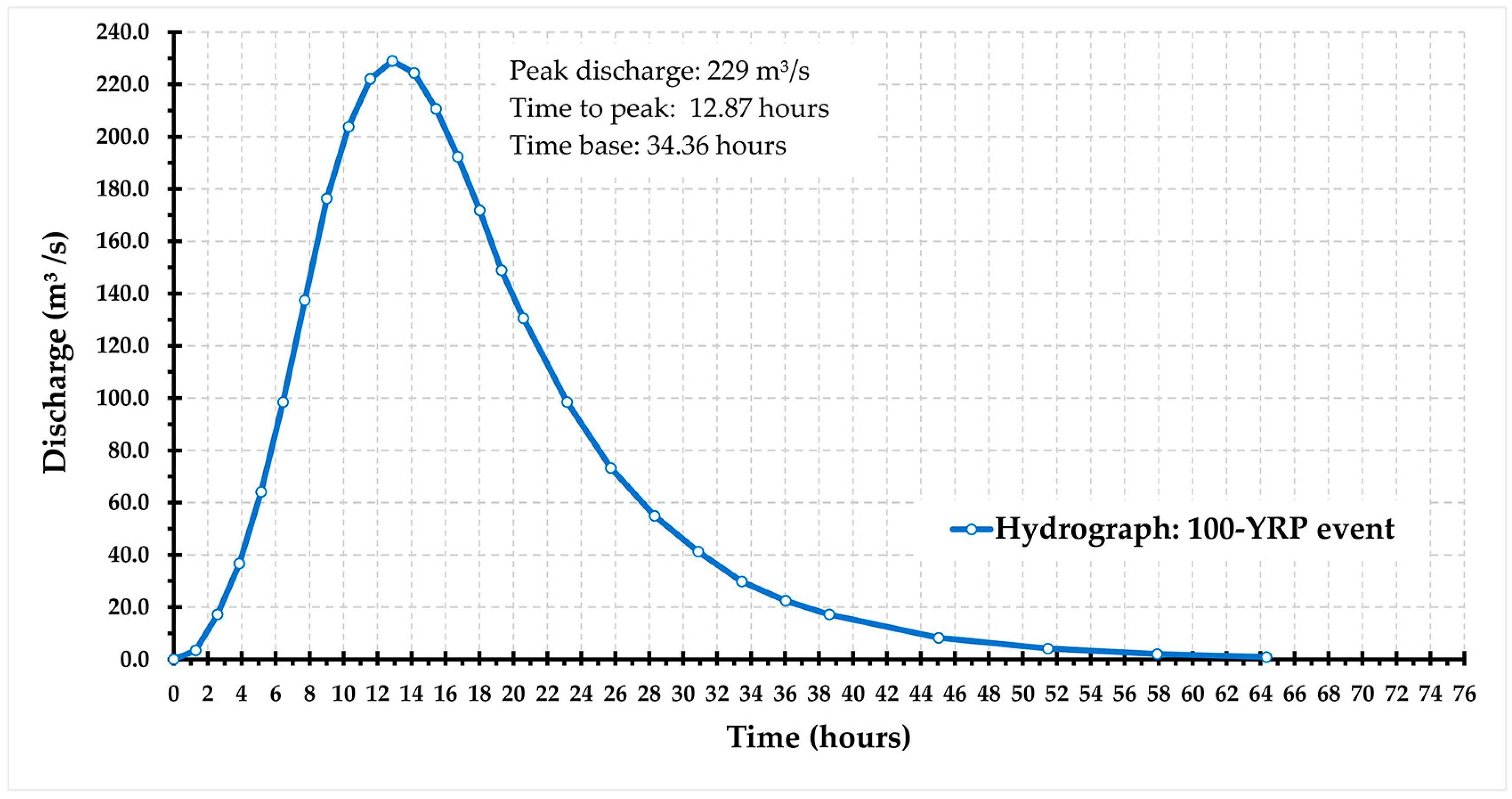
This paper is organized as follows: after this introduction, there is a description of geometrical and hydrological data. The case study and applied methodology is shown in Section 2. Section 3 presents the main experimental results drawn from the research. In Section 4, the results are discussed in detail. Lastly, Section 5 addresses the general conclusions from the study.

2. Materials and Methods

2.1. Geometric Data

Two geometric sources have been taken into account in this research. The first one source is LiDAR-data (from active sensors). Geometric source of National System of Flood Zone Mapping (SNCZI, [59]) were developed due to these data. Nowadays in Spain, two LiDAR-data are available: (a) bare-ground DTM and (b) LiDAR dense point cloud automatically classified. Both data are freely obtained from the National Center for Geographic Information according to INSPIRE Directive [60] and the National Plan for Territory Observation [61].

Table 1. LiDAR data. Geometric characteristics.

Geometric Data	Parameter	Value
Bare-ground DTM	Spatial resolution. Mesh size	5.00 m × 5.00 m
	Vertical precision.	±0.50 m
Dense Point Clouds	Spatial resolution. Point density.	0.5 point m−2
	Average distance between points.	1.41 m
	Vertical uncertainty. RMSE(Z) 1	±0.20 m

¹ RMSE (Z): Root mean square error (vertical).

summarizes the geometric characteristics of both LiDAR-data.

The second data source is an accurate-high resolution and ad hoc dense point cloud (XYZ coordinates with RGB values), which was obtained by RC-APP methodology. This is an efficient (time-cost) approach based on photogrammetry and computer vision. This method, through the hybridization of reduced costs passive sensors, on board in alternative aerial platforms type ULM (Ultra-Light Motor), provides accurate and detailed topographic data from digital aerial images to fluvial applications. RC-APP is intensively exposed and detailed in the study Zazo et al. [43].

2.2. Case Study

This study is located in the upper basin of the Adaja River, which is a sub-system integrated into the Duero river basin known as the largest river basin in the Iberian Peninsula (Figure 1). Study area comprises ≈(1.5 km × 0.8 km), focusing attention on a peri-urban area of ≈(1.3 km × 0.6 km) in the municipality of El Fresno, where it also located a bridge.

The flow regime is natural and river reach is characterized by a well-defined river bed of sand and gravel with an average width of 80 m and two wide and regular floodplains that are each of 250 m in width approximately. Likewise, there are specific areas of dense trees and riverbank vegetation. The sinuosity is low (s = 1.11, 1 < s < 1.3, [40]) with a length of thalweg of 1402 m and in a straight-line of 1268 m (Figure 1).

Regarding the sub-basin of 530 km², its time of concentration (Tc) is 11.7 hours (h) according to the legal requirement in Spain. This provides an assessment of level exposure as “severe” (1 h < Tc < 12 h, [49]) from a security point of view. Furthermore, the Adaja sub-basin shows a scarce and irregular rainfall, which leads to long dry periods that enable total inspection of the riverbed.

2.3. Hydrological Data

A 100-year return period (100-YRP) flow of 229 m³ s⁻¹ was simulated. This is an accepted and common design flow applied to the flood hazard [24,62]. This flow value was supplied by the Duero River Basin Authority through a map of instant peak flows in the natural regime [63]. According to previous work in the area Zazo et al. [42,43], this flow does not provide relevant consequences neither in the bridge zone nor in the urban area. In contrast, the floodplain is significantly affected because the carrying capacity of the main channel is considerably exceeded.

Regarding the map of instant peak flows, this is obtained through maximum discharges time series records of gauging stations related to the peak flood flow with its annual probability of occurrence (quantile or frequency law). This is done by analyzing six different YRP (2, 5, 10, and 25, 100, and 500 years). Through a process of consistency validation of the time series (reliability of records, time tendency check by Mann-Kendall test, and outliers data, mainly), the gauging of peak flows is adjusted to a generalized extreme values distribution function by the L-moments method. Previously, Spanish peninsular river basins are split into homogeneous regions through geographical criteria based on the orography of the basin, the altitude, the rainfall patterns, and the value of the highest precipitation quantiles. This split is subsequently checked by statistical homogeneity tests such as Wiltshire and Hosking-Wallis tests.

Flow assessment at sites that have no gauging station is carried out by an extrapolation of results. In the case of basins larger than 500 km², the extrapolation process is carried out by statistical multiple regression models that relate the quantiles of gauging stations or specific statistics with physiographic and climatic characteristics of the basin. For sub-basin lower than 500 km², hydro-meteorological models are applied. For a more deep explication on the generation process of this map, the reader is referred to the work CEDEX [64].

The instant map value is transformed into unsteady flow by the Soil Conservation Service (SCS) dimensionless unit hydrograph [65]. According to the exposed aim (Section 1) and the eminently geomatic context in which this work is developed, this flow hypothesis is valid. Figure 2 shows the resulting inflow hydrograph.

2.4. Methodology

This research is articulated in four stages (Figure 3). First, an accurate-high resolution dense point cloud is obtained by the RC-APP methodology. From this initial data, different point clouds were derived in which each of them had a different point density (Stage-1). Then, the vegetation influence was reduced through a novel point cloud filter based on the cloth simulation technique. After that, DTMs were generated and their vertical uncertainties were assessed by a variant of a non-parametric RE method (Stage-2). Next, 2D hydraulic simulations were performed with the same set of hydraulic parameters (except DTMs, Stage-3). Lastly, flood modeling and hazard assessment were assessed and compared in-depth against the results achieved that were supported by LiDAR-DTMs (Stage-4).

2.4.1. Stage-1. Data Acquisition. Point Cloud by Means of RC-APP Methodology

At this stage, DP-data acquisition is entirely done by RC-APP methodology. Because of dry conditions, it was not necessary to bathymetric techniques. RC-APP comprises: (a) an unconventional manned aerial platform ULM type (Ultra-Light Motor), (b) gyro-stabilized cameras platform MultiSpectral Airborne System (MUSAS^®), and (c) a simple hand-held digital camera, reflex type (non-photogrammetric camera). Thus digital aerial images (data-set) are acquired. Next, by means of a photogrammetric and computer vision process through a Structure from Motion (SfM) algorithm, supported by Agisoft PhotoScan^® software in this case, aerial images were processed and the high spatial resolution dense point cloud was obtained. Furthermore, it should be noted that a Global Navigation Satellite System (GNSS) observation was also needed: (1) to geo-reference DP-data via 12 Ground Control Points (GCP) located on artificial targets and (2) to assess DTM-vertical uncertainty through 56 Check Points situated on natural features.

ULM and MUSAS^® platforms are widely described in Ortega-Terol et al. [66]. Flight parameters and constraints were the same as that in previous research studies in the zone [42,43] because of the optimal ratio (accuracy-spatial resolution) achieved. In addition, it should be noted that meteorological conditions could constraint flight planning. In this sense, weather requirements would comprise aspects such as minimum wind speed, the absence of rain, or the presence of turbulence resulting from thermal currents among others [66]. In the case of the mini-trike, the recommended wind speed should be lower than 15 km/h. Furthermore, regarding image quality, low illumination conditions could generate blurring effects. However, the MUSAS^® gyro-stabilized platform minimizes this issue. To a complete discussion of photogrammetric and computer vision process and SfM background, it refers the reader to Fonstad et al. [67], Hartley and Zisserman [68], and Snavely [69].

Table 2. Technical specifications: sensor and flight.

	Parameter	Value
Sensor	Camera model	Canon EOS 5D Mark II
	Sensor type/size	CMOS/36 × 24 mm
	Image size	5616 × 3744 pixels
	Pixel size	6.41 × 10−3 mm
	Focal length	50 mm
	Exposure time	1/800 s
Flight	ULM platform. Speed:	11 m s−1
	Flight height	200 m (above ground level)
	Cover area	146 × 97 m/aerial image
	GSD 2	0.026 m

² GSD: Ground Sample Distance (pixel size on the ground).

summarizes the main technical specifications both the sensor used as well as the flight performed.

Table 3. Point clouds: Density points initial.

Point Cloud	Point Density/Spatial Resolution (m × m)
DP-100 3	≈100 point m−2/≈(0.10 × 0.10) m
DP-45	≈45 point m−2/≈(0.15 × 0.15) m
DP-15	≈15 point m−2/≈(0.25 × 0.25) m
DP-5	≈5 point m−2/≈(0.45 × 0.45) m
DP-0.50	≈0.5 point m−2/≈(1.41 × 1.41) m

³ DP-100: Initial point cloud from the RC-APP technique.

shows point clouds obtained from the initial RC-APP point cloud.

2.4.2. Stage-2. DTM Generation and Vertical Assessment

Having a reliable and continuous DTM is essential for flood modeling properly [41,42,58,70]. Likewise, the influence of an accurate and detailed terrain on hydraulic simulations and flood modeling is well known [51,57,71]. Some studies have demonstrated how minor errors have consequences on hydraulic model results [43,45,62]. In this sense, the terrain representation may also be adversely affected by the effects of vegetation due to ground concealment, overestimation of ground surface elevation, and sudden changes in the ground surface among others [72,73,74,75]. Accordingly, given that a DTM is derived by interpolation of the points belonging to the bare earth surface, it is crucial to accurately classify point clouds into ground/non-ground through a filtering process. For this reason, a novel, robust, and easy-to-set point cloud filter named Cloth Simulation Filtering (CSF) was applied to RC-APP point clouds (Table 3). This point filtering process raised a double challenge: on one side, to preserve the geometrical structure of the elements existing on the floodplain (stone masonry, walls, and constructions) that channel and constrain the flow, and, on the other, to apply a filter designed initially to operate with LiDAR-data whose spatial resolution is far less than the RC-APP point cloud.

CSF is based on simulating the colocation of a piece of “cloth” with certain rigidity over an inverted point cloud. The cloth is simulated through an interconnected particles grid through a cloth simulation technique [76]. The main CSF steps are: (1) the initial point cloud is inverted upside-down and, over that, a new inverted surface of the cloth with rigidness is extended, (2) the cloth-shape is adjusted through functions that explained gravity (Newton’s second law) and forces of interaction between particles on the cloth (Hooke’s law), (3) the classification in ground/non-ground points is carried out by cloth particle types (unmovable/movable), and (4) a post-processing method is applied to address abrupt terrain changes. For further discussion, it refers the reader to Reference [58].

The CSF filter is setup by nine parameters: (i) three points shift (X,Y,Z) that do not need setup generally, (ii) one steep slope fit factor (0 flat terrain, 1 steep slopes), (iii) cloth rigidness value (1, 2, or 3), (iv) a time step parameter, which handles the influence of gravity in each iteration (default 0.65), (v) maximum iteration times of simulation, (vi) a class threshold that aids the identification of ground points, and (vii) a cloth resolution or particle separation that implies particles creating. This algorithm is implemented in open source free software CloudComparer^®. However, when the point cloud has a high-spatial resolution, as seen in the RC-APP case, this software cannot process them. For that, the CSF algorithm was implemented in a numerical computing environment like MATLAB^®.

From bare-ground point clouds, the different DTMs were generated by Triangulated Irregular Networks, which were subsequently transformed to 2.5-D (raster) models by applying the linear method as an interpolation choice.

On the other hand, one of the key factors to carry out a reliable flood modeling is to know DTM-vertical uncertainty [43,44,77,78]. Here, a variant of the RE method is proposed [42], which does not require a priori knowledge of the errors distribution function and, therefore, normality tests are not necessary. According to Rodriguez-Gonzalvez et al. [79,80], the central tendency of vertical errors is determined by a median and its statistical dispersion is properly evaluated through a Normalized Median Absolute Deviation (NMAD, [81]). This new proposed evaluation is expressed below.

$$MAD=m\left(\left|x_i-m_x\right|\right)$$

(1)

$$NMAD=1.4826·MAD$$

(2)

where MAD is the Median Absolute Deviation (Equation (1)), m is the median of the absolute deviations from the data’s median, and NMAD is the Normalized Median Absolute Deviation (Equation (2)). This approach allows the statistical dispersion vertical-DTM error to be comparable with the concept of standard deviation of a normal distribution.

2.4.3. Stage-3. Hydraulic Model

Currently, there are a wide availability of numerical tools for one and two dimensional (1D/2D) and 1D/2D coupled hydrodynamic modeling based on the fully-dynamic wave modeling. These tools provide accurate predictions of the hydraulic behavior of flood flow. Some of them are free while others require a license purchase [38]. To a conceptual review of hydrodynamic modeling packages, its numerical schemes, capabilities, and applications, the reader is referred to Patel et al. [82], Weber [83], and Néelz and Pender [84] because a full review of these models is not appropriate for an eminently geomatic manuscript.

Regarding free software, one of the most widely used hydraulic models is HEC-RAS^® [28,38] and was developed by the U.S. Army Corps of Engineers (USACE). Traditionally, it was just a 1D hydraulic model. However, it was successfully applied to flood modeling research [62,70,85,86,87,88,89,90,91]. Recently, HEC-RAS^® has been updated to version 5 and has implemented a fully 2D flow routing within the unsteady flow analysis through a closed polygon that is split into computation cells of up to 8 sides. Now, HEC-RAS^® v5 can perform completely 1D and 2D unsteady flow simulations or combined 1D/2D modeling called hybrid models through the interconnection of both. The program can also solve the full version of 2D Saint-Venant equations or the 2D Diffusion Wave (DW) equations [92].

This new numerical tool is gaining attention among researchers who are highlighting current works such as References [11,38,93]. Liu et al. [11] evaluates the influence of the hydraulic models and surface roughness on flood modeling by four usually used 1D and 2D hydraulic models (HEC-RAS^® 1D and 2D through 2D Saint-Venant equations, LISFLOOD-FP^® diffusive and subgrid). In Moya Quiroga et al. [38], the applicability of HEC-RAS^® v5 to flood modeling using DW equations is studied. On the other hand, Moya Quiroga et al. [93], also using DW equations implemented in HEC-RAS^® v5, analyzes the importance of flood duration by comparing flood hazard maps based on flood depth with flood hazard maps by considering flood duration.

It is important to underline that bed friction and terrain are dominant aspects [37] especially on the floodplain. Additionally, it is remarkable that the strong geomatic component of this research focuses exclusively on the influence of the DTM spatial resolution and vertical uncertainty. For that, 2D DW equations approximations were applied in this work using software version 5.0.3. These equations are valid in the case of slowly evolving floods and overflows [93,94] (as it happens in this study, please see Section 2.2 floodplain description and Section 2.3 inflow hydrograph). In addition, the application of this numerical scheme is characterized by more efficient hydraulic simulations computationally [37,38,93].

As a method to solve the equations, the implicit finite volumes algorithm is used. This provides an increment of improved stability and robustness over usual methods such as finite differences or finite elements. Furthermore, the wetting and drying of computational cells is robust and 2D flows areas can start completely dry [92]. 2D flow computational mesh was defined by an irregular polygon, ≈(1.3 km × 0.6 km), which was mainly split into square cells. Boundary cells had an irregular shape between 3 up to 8 sides.

The numerical scheme was controlled by the relationship among the time step (Δt; seconds) and the size cell (Δx; meters). To avoid numerical instability into the hydraulic model, Δt and Δx was selected, according to the Courant-Friedrichs-Levy condition (Courant number—C).

$$C=\frac{c·\Delta t}{\Delta x}\le 1.0=\frac{\left(\sqrt{g·h}\right)·\Delta t}{\Delta x}\le 1.0$$

(3)

where c is the flood wave velocity or wave celerity (m s⁻¹), g is the gravity acceleration (m s⁻²), and h is the flow depth (m). The celerity c was estimated based on the maximum observed water depth (3.03 m) in the area to the same water flow of 100-YRP (see Zazo et al. [42]). Furthermore, for 2D flow computational meshes that star dry simulation (Section 2.3), it is recommended to use a time step based on a Courant number of 1.0 to get a more accurate and stable wetting front [92].

Since boundary conditions were used: (i) upstream: inflow SCS-hydrograph (Section 2.3) and (ii) downstream: rating curve according to Zazo et al. [42] results (please note that the same downstream boundary was used in both works). The roughness coefficient “n” was selected after a calibrated process based on the inundated area for 100-YRP flow from SNCZI and the results of preceding studies in the zone [42,43].

Table 4. Hydraulic model. Main data.

Parameter	Value
Δt	4 s 4
Δx	21.5 m
n (main channel)	0.035
n (floodplain)	0.015 (road), 0.10 (woodland), 0.05 (riverbank) 10 (building, piers-abutments), 0.035 (rest of cases)
Hydrograph	SCS dimensionless unit hydrograph (Section 2.3)
Water flow (100-YRP)	Peak discharge 229 m3 s−1, Time base: 34. 36 h
Geometric basis	DTMs (Section 2.4.2)

⁴ According to Equation (3), and Courant number equal to 1. Please note that the hydraulic cells have a higher mesh size than any of the spatial resolutions of the DTMs considered in this research (see Table 3).

summarizes the main data of the hydraulic model.

Given that the version of the software used does not support bridge modeling capabilities inside of a 2D flow area, the bridge was modeled by high Manning’s roughness coefficients that simulated the influence of piers and abutments. Exclusively, if the lower part of the bridge deck was affected, a hybrid model 1D/2D was defined. This model consists of a 1D model in the bridge area, defined by a cross section [95], that is connected to two 2D flow computational meshes (upstream and downstream, respectively).

2.4.4. Stage-4. Flood Hazard Assessment

This last stage is crucial in the proposed methodology. Once executed and calibrated as the first hydraulic simulation, which is supported by the highest spatial resolution DTM, the unique variable that was modified in the following simulations was the basic geometrical model (DTMs generated in Stage-2 and DTMs-LiDAR indicated in Section 2.1). All other parameters of the hydraulic model were kept fixed. In this way, the differences both on flood modeling and the hazard assessment will be exclusively produced by the spatial resolution of DTMs and their vertical uncertainties.

Flood hazard assessment was carried out considering the Spanish guidelines for flood prone areas of fluvial origin [49]. MAGRAMA [49] is based on the European Union Floods Directive [24] and it is in line with Martin Vide [40] regarding depth/velocity–damage curves at rural and peri-urban environments and the arguments of Milanesi et al. [22] in relation to combination of flow depths, velocities, and vulnerability curves to assess the flood hazard properly. Furthermore, the target area was focused on the floodplain because the main channel itself is a well-known high-hazard zone [49].

The process of assessment, in each hydraulic simulation, was based on three key factors from the safety standpoint: (1) response time of the basin to a flood (Tc), (2) the maximum inundated area, and (3) the maximum flood depths and velocities achieved simultaneously was associated with the maximum flood. According to MAGRAMA [49],

Table 5. Hydraulic parameters. Threshold values.

Level Exposure	Parameter
Severe 1 h < Tc < 12 h	Flood Depth (D) > 1 m or
	Velocity (V) > 1 m s−1 or
	D × V > 0.5 m−2 s−1

shows the threshold values of hydraulic parameters to hazard assessment. Other aspects such as flow erosive capacity transported solid flow and geological hazards, which were not considered due to the geomatic framework of this work.

It is worth noting the role that Tc plays. In this sense, it is well known that level exposure increases as Tc decreases as well as this factor that informs the available time to take the appropriate measures to minimize the possible damages [49]. For that, the analysis of the flood hazard was focused on threshold hydraulic parameters, according to Tc.

From each hydraulic model, a set of vector maps of the maximum values of thresholding hydraulic variable will be available in addition to the maximum flood area (Stage 2.4.3). Then, all enclosures and lines of these vector maps will be intersected with each other for generating the flood hazard map associated with each DTM. This cartographic process as well as the comparison of the results (RC-APP-data versus LiDAR-data) was supported through the open source Geographical Information System software QGIS.

3. Results

3.1. Bare-Ground DTM Generation and Vertical Assessment

By using a training process on nine CSF parameters, an optimum set of parameters was found, which allowed a suitable classification of points (ground/non-ground points) while keeping the geometric structure of the floodplain elements such as stone masonry, walls, and constructions. Consequently, the most appropriate values were: steep slope fit factor = 1, cloth rigidness = 3, time step = 0.65, iterations = 1000, class threshold = 0.70 (in all cases), and cloth resolution = the same value that point density from the DP-data (see

Table 6. Point clouds: Density points initial.

DP Initial Data 4		CSF Filter. Points Clasiffication		Final DTMs
		Bare-Ground	Non Ground
	Points ≈ Density Points			Mesh Size
DP-100	88,943,111 ≈ 111 point m−2	84,822,510 ≈ 106 point m−2	4,120,601 ≈ 5 point m−2	0.10 m × 0.10 m
DP-45	38,612,537 ≈ 48 point m−2	36,343,108 ≈ 45 point m−2	2,269,429 ≈ 3 point m−2	0.15 m × 0.15 m
DP-15	13,062,459 ≈ 16 point m−2	12,195,988 ≈ 15 point m−2	866,471 ≈ 1 point m−2	0.25 m × 0.25 m
DP-5	4,134,028 ≈ 5 point m−2	3,824,882 ≈ 5 point m−2	309,146 ≈ 0.1 point m−2	0.45 m × 0.45 m
DP-0.5	413,011 ≈ 0.5 point m−2	366,603 ≈ 0.5 point m−2	46,408 ≈ 0.1 point m−2	1.41 m × 1.41 m

⁴ Case study area: ≈800,000 m².

). From bare-ground density points, different 2.5-D DTMs were generated through a conservative adjustment process. Table 6 summarizes the results achieved (bare-ground/non ground) and the final mesh sizes obtained for the geometrical models that will be used in the hydraulic simulations. Please note that the influence of the geometrical structure of the existing constructions is addressed through both point density (mesh size DP-data) and the CSF filter to get reliable DTMs.

As mentioned in (Stage-2), from 56 check points belonging to GNSS observation, with a vertical precision (RMSE_(Z)) of (0.014 ± 0.002) m and applying the Equations (1) and (2), the vertical uncertainty of DTMs was assessed.

Table 7. Vertical uncertainties of DTMs through the RE method.

DTMs 5	Central Tendency (median)	Statistical Dispersion		Vertical Uncertainty
		MAD	NMAD
0.10 m × 0.10 m	0.00 m	0.04 m	0.06 m	(0.00 ± 0.06) m
0.15 m × 0.15 m	−0.01 m	0.04 m	0.06 m	(−0.01 ± 0.06) m
0.25 m × 0.25 m	0.00 m	0.05 m	0.07 m	(0.00 ± 0.07) m
0.45 m × 0.45 m	0.00 m	0.05 m	0.08 m	(0.00 ± 0.08) m
1.41 m × 1.41 m	−0.02 m	0.05 m	0.08 m	(−0.02 ± 0.08) m

⁵ Mesh size.

shows the obtained results through an exposed method. Subsequently, in Section 3.3, these uncertainty values from DP-DTMs will be compared with the vertical precision/uncertainty of the LiDAR-data (Table 1).

3.2. Influence of the DTM Mesh Size on Flood Modeling and a Hazard Assessment

First, Figure 4 shows the cartographic process of generating the hazard map from the individual vector maps (see Section 2.4.4).

The effect both of spatial resolution and vertical uncertainty on flood modeling and hazard assessment is highlighted in

Table 8. Influence of mesh size and vertical uncertainty.

Mesh Size	Vertical Uncertainty	Flood Modeling	Hazard Assessment
0.10 m × 0.10 m	(0.00 ± 0.06) m	370,748 m2	108,830 m2
0.15 m × 0.15 m	(−0.01 ± 0.06) m	328,953 m2	105,619 m2
0.25 m × 0.25 m	(0.00 ± 0.07) m	315,991 m2	103,859 m2
0.45 m × 0.45 m	(0.00 ± 0.08) m	308,144 m2	98,911 m2
1.41 m × 1.41 m	(−0.02 ± 0.08) m	311,701 m2	99,950 m2

and Figure 5 and Figure 6.

Figure 7 shows the influence of the DTMs mesh sizes on hydraulic simulations as a consequence of the existing bridge modeling. This figure clearly reveals an affection to the lower part of the bridge deck, which was only observed in the case of the DTM with the highest spatial resolution (0.10 × 0.10 m). This situation led to an increase on the flood depth that comparatively enlarged the flood area (see Table 8).

3.3. Comparison of Results Versus LiDAR Data

To conclude and underline the suitability of the proposed methodology, flood modeling and hazard assessment results were deeply compared with those obtained by a LiDAR technique (see Table 1 LiDAR-DTMs). The Figure 8 and

Table 9. Influence of mesh size and vertical uncertainty.

Mesh Size	Vertical Uncertainty	Flood Modeling	Hazard Assessment
0.10 m × 0.10 m 6	(0.00 ± 0.06) m	370,748 m2	108,830 m2
1.41 m × 1.41 m 6	(−0.02 ± 0.08) m	311,701 m2	99,950 m2
1.41 m × 1.41 m 7	(±0.20) m	290,465 m2	91,100 m2
5.00 m × 5.00 m 7	(±0.50) m	285,835 m2	90,389 m2

⁶ DP-DTM. ⁷ LiDAR-DTM.

show the effects of mesh size and vertical uncertainty on hydraulic simulations. Lastly, Figure 9 summarizes and shows the evolution of the results through normalized area values from Table 8 (DP-data) and Table 9 (LiDAR-data). It can be observed how, as the spatial resolution and vertical uncertainty increase [(from 0.10 m × 0.10 m to 5.00 m × 5.00 m) and (from ±0.06 m to ±0.50 m)], the maximum inundated area and its associated hazard zones decrease. Moreover, based on this figure, it is proposed that the optimal relationship among mesh size (point density) and vertical uncertainty is found in this research.

4. Discussion

The multidisciplinary nature of the flood hazard assessment has led to an active research line within the scientific community. Relevant studies have highlighted the important role that a detailed, continuous, and accurate DTM with a minimal/reduced vegetation influence plays in reliable hydrodynamic modeling results. Although the available spatial resolutions of these DTMs have achieved, so far, in the best case resolutions, to close to one meter and vertical precisions ranged from ±0.50 m and ±0.25 m. For this purpose, the exposed methodology (by RC-APP & CSF) is a novel application because no work has addressed the influence of hyper-resolution DTMs (in the range from ≈1 m to 0.10 m) and with vertical-centimeter uncertainties [from (0.00 ± 0.06) m to (−0.02 ± 0.08)] in the field of flood modeling so far.

It is worth mentioning that the CSF filter reliability as well as the suitability of the parameters set (Section 2.4.2). This is highlighted, on one hand, through the high rates of bare-ground points obtained (among 95.4% and 88.8%, see Table 5) and, on the other hand, the minimal vertical uncertainties achieved (Table 6). This is because DTMs were generated exclusively by bare-ground points. In this sense, the vertical uncertainties, evaluated through the proposed method in this work, ranges among (0.00 ± 0.06) m to DP-100 (0.10 m × 0.10 m mesh size) and (−0.02 ± 0.08) m to DP-0.5 (1.41 m × 1.41 m mesh size). Furthermore, a slight trend towards a high uncertainty in the DTMs was observed as the spatial resolution increases (Table 7). Geometrically, the vertical DP-DTM uncertainties achieved [(0.00 ± 0.06) m and (−0.02 ± 0.08) m, Table 7] ranges roughly among three and seven times better than vertical LiDAR-DTM uncertainties [(±0.20 m and ±0.50 m, Table 1).

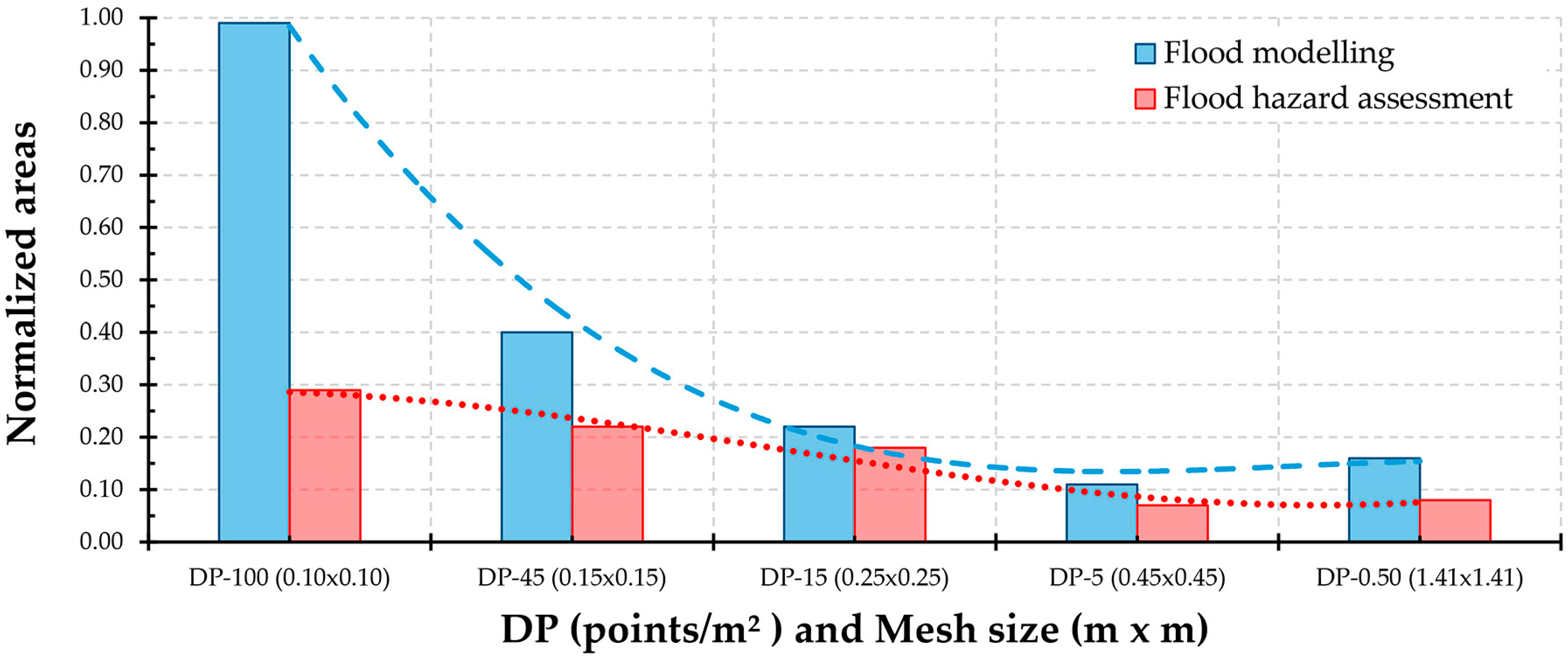
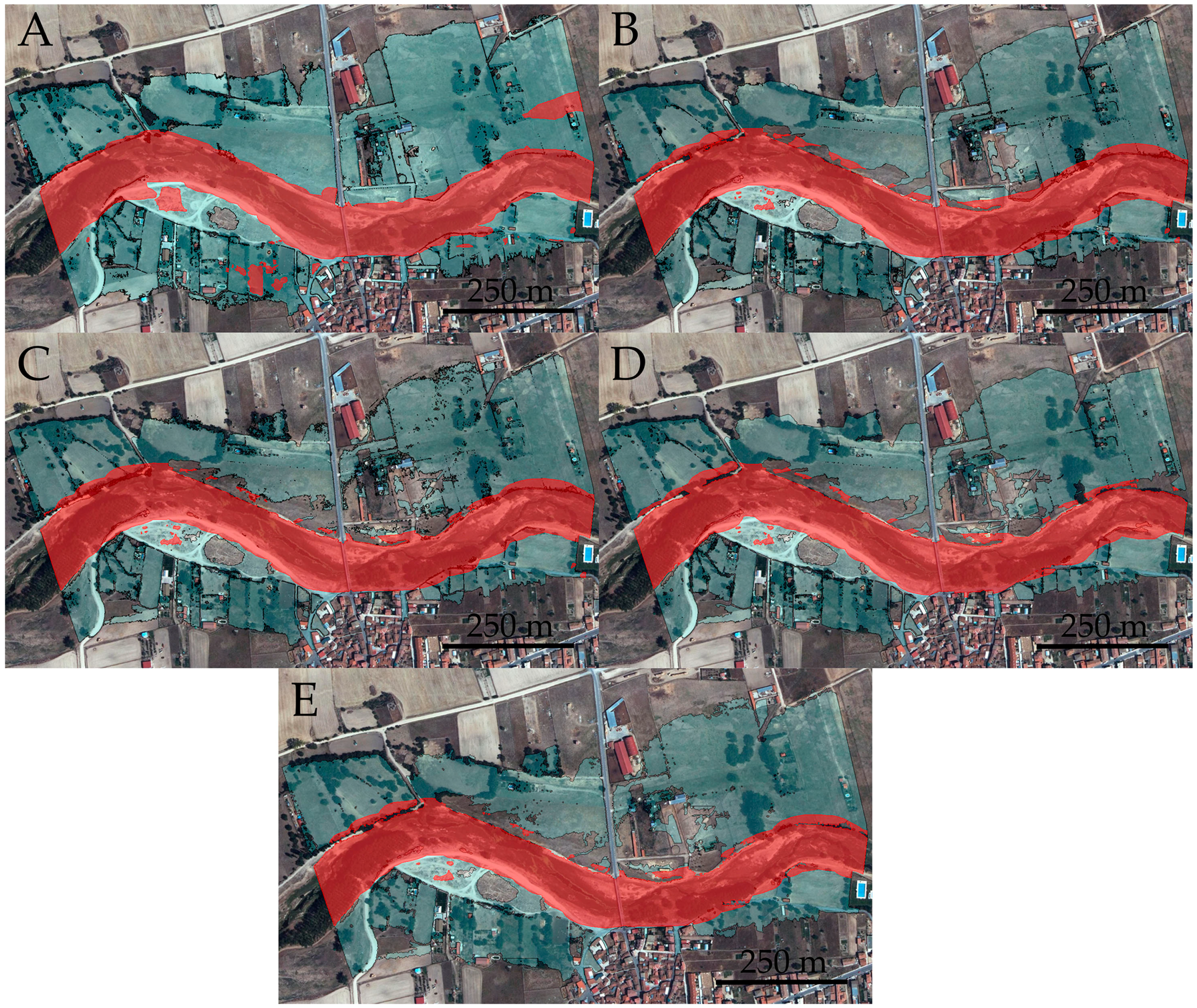
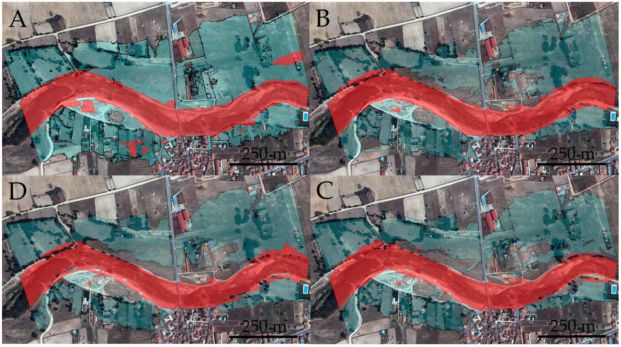
Furthermore, flood modeling shows important differences from the safety point of view (Figure 6). According to DP-100 as a reference value (0.10 m × 0.10 m, 370,748 m², Table 8), the observed differences vary between 15% and 17% for DP-15 (0.25 m × 0.25 m; 315,991 m²) and DP-5 (0.45 m × 0.45 m; 308,144 m²), respectively. It is also observed that the increase of the mesh size (from 0.10 m × 0.10 m to 1.41 m × 1.41 m) produces a decrease on the inundated area (Table 7, 370,748 m² to 308,144 m²). Please note the minimal difference among DP-5 and DP-0.50 (3557 m², 308,144–311,701 m²). However, these differences are increased significantly up to 22% and 23% when the values are compared with LiDAR-data flood modeling (Table 9, 1.41 m × 1.41 m: 290,465 m²; 5.00 m × 5.00 m: 285,835 m²). It should be noted that the minimal difference among LiDAR-data results only in 4630 m² and roughly at 1.6%. In all cases, it is evident the positive effect that a high spatial resolution DTM and low vertical uncertainty has on flood modeling. In this sense, the high density points cloud got by RC-APP & CSF, which have allowed us to obtain DTMs with a large spatial resolution between 50 and 14 times better than LiDAR-data (5.00 m × 5.00 m, 1.41 m × 1.41 m, Table 1).

Next, regarding the hazard assessment (see Table 8), it is noticeable that the higher mesh sizes (0.45 m × 0.45 m and 1.41 m × 1.41 m) do not produce relevant changes (98,911 m² versus 99,950 m², only 1039 m²). However, in the case of lower mesh sizes, there are important variations from a security perspective (108,830 m² 0.10 m × 0.10 m, to 103,619 m² 0.25 m × 0.25 m). The percentages of modification vary between 9% and 5%, respectively. These values can be significant in an area with a high exposure level to the flood hazard. Furthermore, a detailed analysis on Figure 6 shows how there are hazard areas on the floodplain that are only revealed through the maximum resolution DTM (Figure 6: 0.10 m × 0.10 m). This highlights the usefulness of this spatial resolution for drawing up reliable evacuation plans to reduce natural flood hazards. On the other hand, the comparison versus LiDAR-data shows significant differences depending on mesh size, which range between 17%, 108,830 m² and 90,389 m², and 10%, 99,950 m² and 90,389 m² (see Table 9).

Furthermore, it is found that exclusively vertical-DTM uncertainty produces on inundated area and hazard assessment. In Table 9, it is shown that for a mesh size of 1.41 m × 1.41 m, the inundated area varies ≈ 7% [311,701 m², vertical uncertainty of (−0.02 ± 0.08) m, and 290,465 m² (±0.20 m)]. Regarding hazard assessment, the values varies ≈ 9% (99,950 m² and 91,100 m²). This proves that a small difference of only 0.12 m in the vertical uncertainty significantly affects the delimitation of flood modeling and hazard assessment.

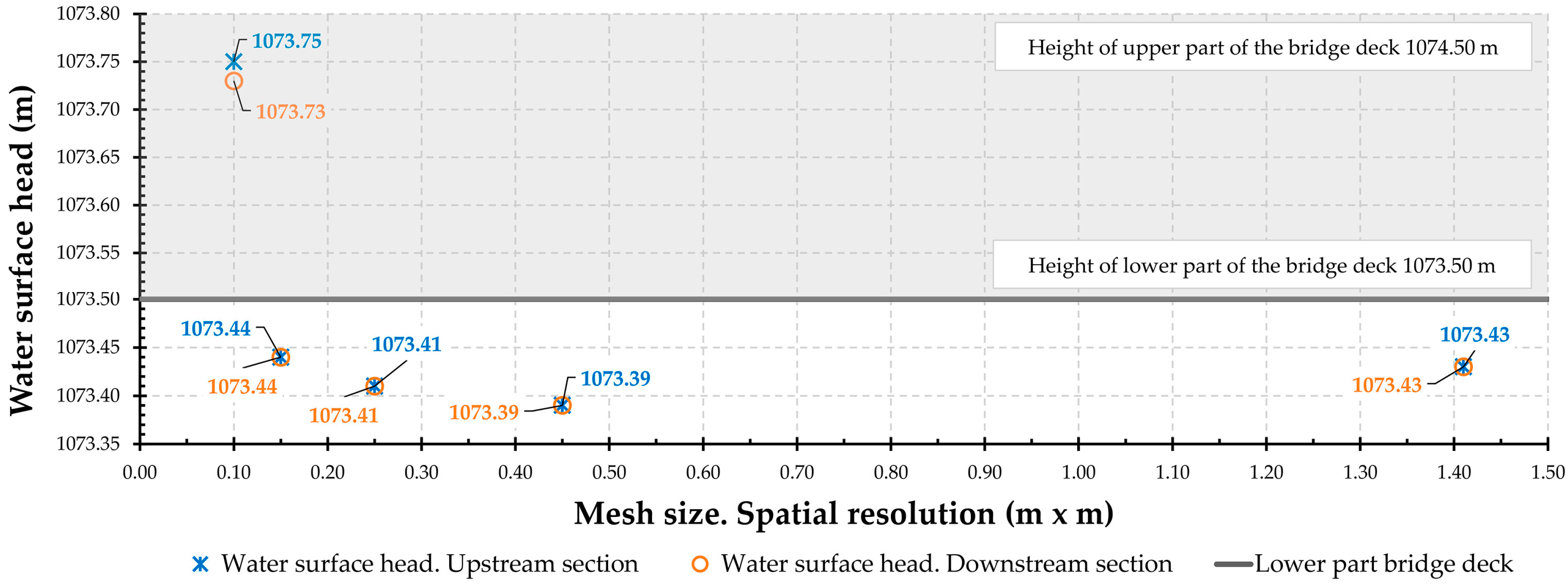
Regarding the existing bridge, Figure 7 shows the influence of the mesh size of DTMs at the bridge area. It should be noted that, only in the case of DP-100 (mesh size of 0.10 m × 0.10 m), water surface elevations higher than the lower part of the bridge deck was detected (1073.50 m). The water surface elevations were 1073.75 m upstream and 1073.73 m downstream. In all other analyzed cases, the achieved values showed a slight variation [1073.39, 1073.44 m] but none of them were higher than 1073.50 m. This clearly shows the positive effect that a high resolution DTM has on flood modeling. In this way, an average difference of 0.32 m on the water surface elevation (1073.39-44 versus 1073.75-73) was found at the bridge area. This situation led to an increase on the flood area and hazard assessment with respect to the other cases studied.

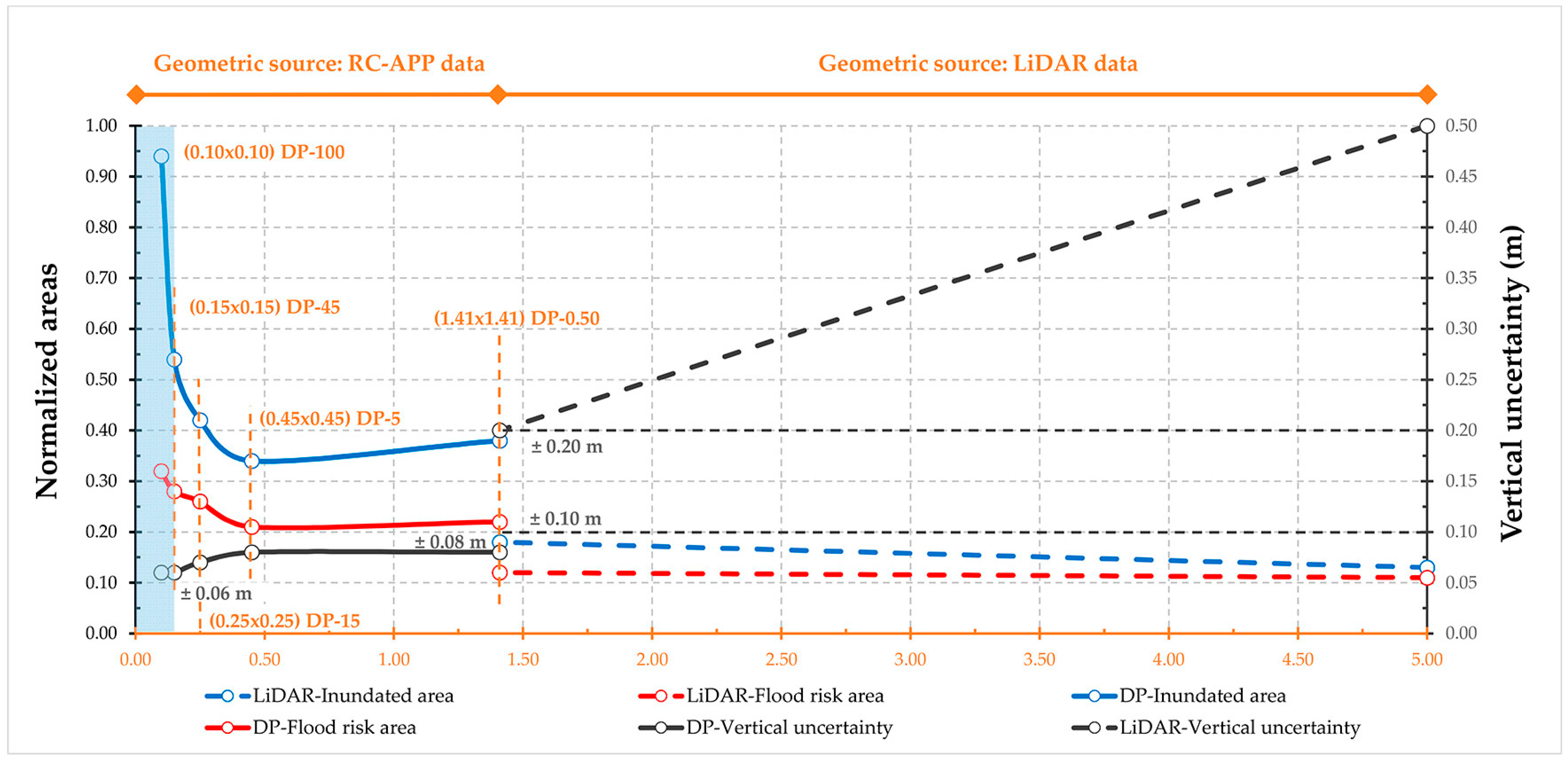
Figure 9 shows the optimal relationship found between the point density and vertical uncertainty. In accordance with it, this research proposes DTMs with a mesh size among (0.10 m × 0.10 m) to (0.15 m × 0.15 m), point densities among 100 to 45-point m⁻² to generate more reliable fluvial hazard maps. Furthermore, through the proposed methodology, it is possible to achieve minimal vertical uncertainties (0.00 ± 0.06) m and (−0.01 ± 0.06) m lower than LiDAR-data commonly applied to fluvial modeling.

Lastly, it should be highlighted that the role of the Manning roughness coefficient is crucial not only for developing accurate flood modeling but also for achieving a deep understanding of the flow regime behavior. From a hazard flood assessment, this analysis is even more important because of the influence that drastic changes in the Manning roughness coefficient may produce on the interaction flow-terrain-infrastructures. To finish, it is also important mentioning that, for upcoming research studies, it was planned to develop a comparative sensitivity analysis of the influence of the Manning roughness coefficient vs. the hydraulic cell size on hydraulic models´ reliability.

5. Conclusions

This study reinforces the suitability analysis of new geomatic solutions as a reliable and competitive source of accurate and high resolutions DTMs. This was done at the service of flood hazard assessment and flood effects mitigation. The proposed methodology has been revealed as an effective strategy of adaptation to deal with the growing variability of the hydrological events and associated systemic risks.

This research has found an optimal relationship between point density (mesh size) and vertical uncertainty. This was done to generate more reliable fluvial hazard maps as well as to improve decision-making in the fluvial framework from the safety perspective. This was developed by minimizing potential flood consequences via more detailed flood prone area maps and making more realistic evacuation plans. In addition, from a technical point of view, flood modeling supported by the proposed methodology would provide a more effective definition of solutions in the field of river engineering as the consequence of a better knowledge of flood behavior. On the other hand, this methodology may also lead to high detailed 4D models applied to morphometry fluvial.

Regarding a comparison with LiDAR-data, this has revealed that a joint approach through both techniques (LiDAR & DP by RC-APP and CSF) would allow a more objective (with less uncertainty) assessment of the inherent river hazard on a specific area. This is found to be even more applicable especially in areas with a high level of flood exposure. This could be performed by LiDAR-data to preliminarily evaluate the potential risks and the exposed methodology in-depth. This joint approach (active/passive sensors, LiDAR versus DP) would allow a better definition of the floodplain land uses, which would reduce the flood hazard.

A setup of technical specifications (sensor and flight) has also been proposed for planning flights by an Ultra-Light Motor but is also applicable to Unmanned Aerial Vehicles. Additionally, the applied methodology (RC-APP and CSF) may be an adequate source of reliable geometric data. This is found to be true not only for fluvial applications but in zones/places where LiDAR-data are not available or with poor quality topographic data. In this sense, the optimal relationship between time-cost achieved a vertical precision-spatial resolution. Furthermore, the application of the CSF algorithm over photogrammetric high resolutions point clouds has been tested and validated. Likewise, the methodology applied to vertical-DTM uncertainty has been demonstrated to be an efficient mode to evaluate vertical accuracy especially in those dataset that do not follow a Gaussian distribution. The exposed method may be applied to DTMs derived from different geometric sources and not only from DP.

For future research, we plan to apply an optimal mesh size and a proposed vertical uncertainty in the form of continuous DTMs. This would be implemented together with the new approaches on hydrological time series analysis such as causal reasoning implemented by the Bayes’ theorem to generate more reliable predictive models on flood modeling.

To conclude, we found that a better knowledge of the interaction flow-terrain through the hybridization of alternative platforms, sensors, and processing techniques (SfM and CSF algorithms) produces a better definition of flood prone areas with important social and economic benefits.

References

1. Chapi, K.; Singh, V.P.; Shirzadi, A.; Shahabi, H.; Bui, D.T.; Pham, B.T.; Khosravi, K. A Novel Hybrid Artificial Intelligence Approach for Flood Susceptibility Assessment. Environ. Model. Softw. 2017, 95, 229–245. [Google Scholar] [CrossRef]
2. Grahn, T.; Nyberg, L. Assessment of Pluvial Flood Exposure and Vulnerability of Residential Areas. Int. J. Disaster Risk Reduct. 2017, 21, 367–375. [Google Scholar] [CrossRef]
3. Macchione, F.; Costabile, P.; Costanzo, C.; De Lorenzo, G.; Razdar, B. Dam Breach Modelling: Influence on Downstream Water Levels and a Proposal of a Physically Based Module for Flood Propagation Software. J. Hydroinform. 2016, 18, 615–633. [Google Scholar] [CrossRef]
4. Jongman, B.; Hochrainer-Stigler, S.; Feyen, L.; Aerts, J.C.J.H.; Mechler, R.; Botzen, W.J.W.; Bouwer, L.M.; Pflug, G.; Rojas, R.; Ward, P.J. Increasing Stress on Disaster-Risk Finance due to Large Floods. Nat. Clim. Chang. 2014, 4, 264–268. [Google Scholar] [CrossRef]
5. Reynard, N.S.; Kay, A.L.; Anderson, M.; Donovan, B.; Duckworth, C. The Evolution of Climate Change Guidance for Fluvial Flood Risk Management in England. Prog. Phys. Geogr. 2017, 41, 222–237. [Google Scholar] [CrossRef]
6. MAGRAMA. Gestión de los Riesgos de Inundación. Available online: http://www.magrama.gob.es/es/agua/temas/gestion-de-losriesgos-de-inundacion/ (accessed on 15 April 2018).
7. Mateo-Lázaro, J. Hidrología de Crecidas en Pequeñas y Medianas Cuencas. Aplicación con Modelos Digitales del Terreno. Ph.D. Dissertation, University of Zaragoza, Zaragoza, Spain, 12 September 2010. [Google Scholar]
8. Arnell, N.W.; Gosling, S.N. The Impacts of Climate Change on River Flood Risk at the Global Scale. Clim. Chang. 2016, 134, 387–401. [Google Scholar] [CrossRef]
9. Gobeyn, S.; Van Wesemael, A.; Neal, J.; Lievens, H.; Van Eerdenbrugh, K.; De Vleeschouwer, N.; Vernieuwe, H.; Schumann, G.J.-P.; Di Baldassarre, G.; De Baets, B.; et al. Impact of the Timing of a SAR Image Acquisition on the Calibration of a Flood Inundation Model. Adv. Water Resour. 2017, 100, 126–138. [Google Scholar] [CrossRef]
10. Rosser, J.F.; Leibovici, D.G.; Jackson, M.J. Rapid Flood Inundation Mapping using Social Media, Remote Sensing and Topographic Data. Nat. Hazards 2017, 87, 103–120. [Google Scholar] [CrossRef]
11. Liu, Z.; Merwade, V.; Jafarzadegan, K. Investigating the Role of Model Structure and Surface Roughness in Generating Flood Inundation Extents using One-and Two-dimensional Hydraulic Models. J. Flood Risk Manag. 2018, e12347. [Google Scholar] [CrossRef]
12. Molina, J.-L.; Zazo, S. Causal Reasoning for the Analysis of Rivers Runoff Temporal Behavior. Water Resour. Manag. 2017, 31, 4669–4681. [Google Scholar] [CrossRef]
13. Molina, J.-L.; Zazo, S. Assessment of Temporally Conditioned Runoff Fractions in Unregulated Rivers. J. Hydrol. Eng. 2018, 23. [Google Scholar] [CrossRef]
14. Molina, J.-L.; Zazo, S.; Rodriguez-Gonzalvez, P.; Gonzalez-Aguilera, D. Innovative Analysis of Runoff Temporal Behavior through Bayesian Networks. Water 2016, 8, 484. [Google Scholar] [CrossRef]
15. Min, S.; Zhang, X.; Zwiers, F.W.; Hegerl, G.C. Human Contribution to More-Intense Precipitation Extremes. Nature 2011, 470, 378–381. [Google Scholar] [CrossRef] [PubMed]
16. Zhang, X.; Wan, H.; Zwiers, F.W.; Hegerl, G.C.; Min, S. Attributing Intensification of Precipitation Extremes to Human Influence. Geophys. Res. Lett. 2013, 40, 5252–5257. [Google Scholar] [CrossRef]
17. O’Gorman, P.A. Precipitation Extremes under Climate Change. Curr. Clim. Chang. Rep. 2015, 1, 49–59. [Google Scholar] [CrossRef] [PubMed]
18. Marotzke, J.; Jakob, C.; Bony, S.; Dirmeyer, P.A.; O’Gorman, P.A.; Hawkins, E.; Perkins-Kirkpatrick, S.; Le Quere, C.; Nowicki, S.; Paulavets, K.; et al. Climate Research must Sharpen its View. Nat. Clim. Chang. 2017, 7, 89–91. [Google Scholar] [CrossRef] [PubMed]
19. Donat, M.G.; Lowry, A.L.; Alexander, L.V.; O’Gorman, P.A.; Maher, N. More Extreme Precipitation in the World’s Dry and Wet Regions. Nat. Clim. Chang. 2016, 6, 508–513. [Google Scholar] [CrossRef]
20. Schiermeier, Q. Increased Flood Risk Linked to Global Warming. Nature 2011, 470, 316–317. [Google Scholar] [CrossRef] [PubMed]
21. Thieken, A.H.; Cammerer, H.; Dobler, C.; Lammel, J.; Schoeberl, F. Estimating Changes in Flood Risks and Benefits of Non-Structural Adaptation Strategies—A Case Study from Tyrol, Austria. Mitig. Adapt. Strateg. Glob. Chang. 2016, 21, 343–376. [Google Scholar] [CrossRef] [PubMed]
22. Milanesi, L.; Pilotti, M.; Ranzi, R. A Conceptual Model of People’s Vulnerability to Floods. Water Resour. Res. 2015, 51, 182–197. [Google Scholar] [CrossRef]
23. Albano, R.; Mancusi, L.; Sole, A.; Adamowski, J. Collaborative Strategies for Sustainable EU Flood Risk Management: FOSS and Geospatial Tools-Challenges and Opportunities for Operative Risk Analysis. ISPRS Int. J. Geo-Inf. 2015, 4, 2704–2727. [Google Scholar] [CrossRef]
24. EU Directive. EU Directive of the European Parliament and the European Council on the Assessment and Management of Flood Risks. (2007/60/EU) 2007. Off. J. Eur. Union 2007, 15, 186–193. [Google Scholar]
25. Williams, K.; Gupta, R.; Hopkins, D.; Gregg, M.; Payne, C.; Joynt, J.L.R.; Smith, I.; Bates-Brkljac, N. Retrofitting England’s Suburbs to Adapt to Climate Change. Build. Res. Inf. 2013, 41, 517–531. [Google Scholar] [CrossRef]
26. Zechner, S.; Grossmann, G.; Pohl, R.; Natale, L.; Escuder Bueno, I.; Bateman, A. Guidance. SUFRI Metodology for Investigation of Risk Awareness of the Population Concerned. 2nd ERA-Net CRUE Funding Initiative European Flood Risk. Available online: https://bit.ly/2DvTEoY (accessed on 27 September 2018).
27. Jonkman, S.N.; Lentz, A.; Vrijling, J.K. A General Approach for the Estimation of Loss of Life due to Natural and Technological Disasters. Reliab. Eng. Syst. Saf. 2010, 95, 1123–1133. [Google Scholar] [CrossRef]
28. Romali, N.S.; Yusop, Z.; Ismail, A.Z. Application of Hec-Ras and Arc Gis for Floodplain Mapping in Segamat Town, Malaysia. Int. J. Geomate 2018, 14, 125–131. [Google Scholar] [CrossRef]
29. De Moel, H.; van Alphen, J.; Aerts, J.C.J.H. Flood Maps in Europe—Methods, Availability and Use. Nat. Hazards Earth Syst. Sci. 2009, 9, 289–301. [Google Scholar] [CrossRef] [Green Version]
30. Faghih, M.; Mirzaei, M.; Adamowski, J.; Lee, J.; El-Shafie, A. Uncertainty Estimation in Flood Inundation Mapping: An Application of Non-Parametric Bootstrapping. River Res. Appl. 2017, 33, 611–619. [Google Scholar] [CrossRef]
31. Huang, Y.; Qin, X. Uncertainty Analysis for Flood Inundation Modelling with a Random Floodplain Roughness Field. Environ. Syst. Res. 2014, 3, 9. [Google Scholar] [CrossRef]
32. Eltner, A.; Kaiser, A.; Castillo, C.; Rock, G.; Neugirg, F.; Abellan, A. Image-Based Surface Reconstruction in Geomorphometry—Merits, Limits and Developments. Earth Surf. Dyn. 2016, 4, 359–389. [Google Scholar] [CrossRef]
33. Fuller, I.C.; Basher, L.R. Riverbed Digital Elevation Models as a Tool for Holistic River Management: Motueka River, Nelson, New Zealand. River Res. Appl. 2013, 29, 619–633. [Google Scholar] [CrossRef]
34. Thompson, C.J.; Fryirs, K.; Croke, J. The Disconnected Sediment Conveyor Belt: Patterns of Longitudinal and Lateral Erosion and Deposition during a Catastrophic Flood in the Lockyer Valley, South East Queensland, Australia. River Res. Appl. 2016, 32, 540–551. [Google Scholar] [CrossRef]
35. Sena Fael, C.M.; Simarro-Grande, G.; Martin-Vide, J.; Cardoso, A.H. Local Scour at Vertical-Wall Abutments Under Clear-Water Flow Conditions. Water Resour. Res. 2006, 42. [Google Scholar] [CrossRef]
36. Sena Fael, C.M.; Lanca, R.; Cardoso, A. Effect of Pier Shape and Pier Alignment on the Equilibrium Scour Depth at Single Piers. Int. J. Sediment Res. 2016, 31, 244–250. [Google Scholar] [CrossRef]
37. Cea, L.; Blade, E. A Simple and Efficient Unstructured Finite Volume Scheme for Solving the Shallow Water Equations in Overland Flow Applications. Water Resour. Res. 2015, 51, 5464–5486. [Google Scholar] [CrossRef]
38. Moya Quiroga, V.; Kure, S.; Udo, K.; Mano, A. Application of 2D Numerical Simulation for the Analysis of the February 2014 Bolivian Amazonia Flood: Application of the New HEC-RAS Version 5. RIBAGUA-Rev. Iberoam. Del Agua 2016, 3, 25–33. [Google Scholar] [CrossRef]
39. Arrighi, C.; Brugioni, M.; Castelli, F.; Franceschini, S.; Mazzanti, B. Flood Risk Assessment in Art Cities: The Exemplary Case of Florence (Italy). J. Flood Risk Manag. 2018, 11, S616–S631. [Google Scholar] [CrossRef]
40. Martín Vide, J. Ingeniería De Ríos, 2nd ed.; Ediciones UPC: Barcelona, Spain, 2009; pp. 27–30, 121–123. ISBN 978-84-8301-900-9. [Google Scholar]
41. Saksena, S.; Merwade, V. Incorporating the Effect of DEM Resolution and Accuracy for Improved Flood Inundation Mapping. J. Hydrol. 2015, 530, 180–194. [Google Scholar] [CrossRef]
42. Zazo, S.; Rodriguez-Gonzalvez, P.; Molina, J.-L.; Hernandez-Lopez, D.; Gonzalez-Aguilera, D. Flood Analysis Supported by Low-Cost Geometric Modelling. River Res. Appl. 2017, 33, 620–631. [Google Scholar] [CrossRef]
43. Zazo, S.; Molina, J.-L.; Rodriguez-Gonzalvez, P. Analysis of Flood Modeling through Innovative Geomatic Methods. J. Hydrol. 2015, 524, 522–537. [Google Scholar] [CrossRef]
44. Falcao, A.P.; Mazzolari, A.; Goncalves, A.B.; Araujo, M.A.V.C.; Trigo-Teixeira, A. Influence of Elevation Modelling on Hydrodynamic Simulations of a Tidally-Dominated Estuary. J. Hydrol. 2013, 497, 152–164. [Google Scholar] [CrossRef]
45. Md Ali, A.; Solomatine, D.P.; Di Baldassarre, G. Assessing the Impact of Different Sources of Topographic Data on 1-D Hydraulic Modelling of Floods. Hydrol. Earth Syst. Sci. 2015, 19, 631–643. [Google Scholar] [CrossRef]
46. Schanze, J.; Hutter, G.; Olfert, A.; Penning-Rowsell, E.C.; Parker, D.; Harries, T.; Nachtnebel, H.; Holzmann, H.; Neuhold, C.; Meyer, V. Systematisation, Evaluation and Context Conditions of Structural and Non-structural Measures for Flood Risk Reduction; CRUE Research Report No. I-1; CRUE Funding Initiative on Flood Risk Management Research: London, UK, 2008.
47. Escuder-Bueno, I.; Castillo-Rodriguez, J.T.; Zechner, S.; Joebstl, C.; Perales-Momparler, S.; Petaccia, G. A Quantitative Flood Risk Analysis Methodology for Urban Areas with Integration of Social Research Data. Nat. Hazards Earth Syst. Sci. 2012, 12, 2843–2863. [Google Scholar] [CrossRef] [Green Version]
48. Albano, R.; Mancusi, L.; Sole, A.; Adamowski, J. FloodRisk: A Collaborative, Free and Open-Source Software for Flood Risk Analysis. Geomat. Nat. Hazards Risk 2017, 8, 1812–1832. [Google Scholar] [CrossRef]
49. MAGRAMA. Guía Técnica de Apoyo a La Aplicación Del Reglamento Del Dominio Público Hidráulico en Las Limitaciones a Los Usos Del Suelo en Las Zonas Inundables Se Origen Fluvial; Ministerio de Agricultura, Alimentación y Medio Ambiente. Gobierno de España: Madrid, España, 2017.
50. Merz, B.; Elmer, F.; Kunz, M.; Muehr, B.; Schroeter, K.; Uhlemann-Elmer, S. The Extreme Flood in June 2013 in Germany. Houille Blanche-Revue Internationale De L Eau 2014, 5–10. [Google Scholar] [CrossRef]
51. Casas, A.; Benito, G.; Thorndycraft, V.R.; Rico, M. The Topographic Data Source of Digital Terrain Models as a Key Element in the Accuracy of Hydraulic Flood Modelling. Earth Surf. Process. Landf. 2006, 31, 444–456. [Google Scholar] [CrossRef]
52. Molina, J.-L.; Rodriguez-Gonzalvez, P.; Carmen Molina, M.; Gonzalez-Aguilera, D.; Espejo, F. Geomatic Methods at the Service of Water Resources Modelling. J. Hydrol. 2014, 509, 150–162. [Google Scholar] [CrossRef]
53. Horritt, M.S.; Bates, P.D. Effects of Spatial Resolution on a Raster Based Model of Flood Flow. J. Hydrol. 2001, 253, 239–249. [Google Scholar] [CrossRef]
54. Aguilar, F.J.; Mills, J.P. Accuracy Assessment of Lidar-Derived Digital Elevation Models. Photogramm. Rec. 2008, 23, 148–169. [Google Scholar] [CrossRef]
55. Yan, K.; Di Baldassarre, G.; Solomatine, D.P. Exploring the Potential of SRTM Topographic Data for Flood Inundation Modelling Under Uncertainty. J. Hydroinform. 2013, 15, 849–861. [Google Scholar] [CrossRef]
56. Tsubaki, R.; Fujita, I. Unstructured Grid Generation using LiDAR Data for Urban Flood Inundation Modelling. Hydrol. Process. 2010, 24, 1404–1420. [Google Scholar] [CrossRef]
57. Zazo, S. Analysis of the Hydrodynamic Fluvial Behaviour through Causal Reasoning and Artificial Vision. Ph.D. Thesis, University of Salamanca, Ávila, Spain, 12 May 2017. [Google Scholar]
58. Zhang, W.; Qi, J.; Wan, P.; Wang, H.; Xie, D.; Wang, X.; Yan, G. An Easy-to-use Airborne LiDAR Data Filtering Method Based on Cloth Simulation. Remote Sens. 2016, 8, 501. [Google Scholar] [CrossRef]
59. MAGRAMA. Guía Metodológica para el Desarrollo del Sistema Nacional de Cartografía de Zonas Inundables; Ministerio de Agricultura, Alimentación y Medio Ambiente. Gobierno de España: Madrid, España, 2011; pp. 19–33.
60. MFOM. Infraestructura de Datos Espaciales de España. Available online: http://www.idee.es/web/guest/europeo-inspire (accessed on 11 April 2018).
61. IGN. Instituto Geográfico Nacional de España. Available online: http://www.ign.es/PNOA/presentacion.html (accessed on 28 April 2018).
62. Cook, A.; Merwade, V. Effect of Topographic Data, Geometric Configuration and Modeling Approach on Flood Inundation Mapping. J. Hydrol. 2009, 377, 131–142. [Google Scholar] [CrossRef]
63. CEDEX. Mapa de Caudales Máximos Instantáneos en Régimen Natural Asociados a Distintos Periodos de Retorno CAUMAX; Centro de Estudios y Experimentación de Obras Públicas: Madrid, España, 2013. [Google Scholar]
64. CEDEX. Memoria Técnica. Mapa de Caudales Máximos; Centro de Estudios y Experimentación de Obras Públicas: Madrid, España, 2011. [Google Scholar]
65. SCS. Soil Conservation Service—National Engineering Handbook, Section 4, Hydrology; Department of Agriculture, Soil Conservation Service: Washington, DC, USA, 1972.
66. Ortega-Terol, D.; Moreno, M.A.; Hernandez-Lopez, D.; Rodriguez-Gonzalvez, P. Survey and Classification of Large Woody Debris (LWD) in Streams using Generated Low-Cost Geomatic Products. Remote Sens. 2014, 6, 11770–11790. [Google Scholar] [CrossRef]
67. Fonstad, M.A.; Dietrich, J.T.; Courville, B.C.; Jensen, J.L.; Carbonneau, P.E. Topographic Structure from Motion: A New Development in Photogrammetric Measurement. Earth Surf. Process. Landf. 2013, 38, 421–430. [Google Scholar] [CrossRef]
68. Hartley, R.; Zisserman, A. Multiple View Geometry in Computer Vision, 2nd ed.; Cambridge University Press: Cambridge, UK, 2004. [Google Scholar]
69. Snavely, N. Scene Reconstruction and Visualization from Internet Photo Collections. Ph.D. Thesis, University of Washington, Seattle, WA, USA, 2008. [Google Scholar]
70. Merwade, V.; Cook, A.; Coonrod, J. GIS Techniques for Creating River Terrain Models for Hydrodynamic Modeling and Flood Inundation Mapping. Environ. Model. Softw. 2008, 23, 1300–1311. [Google Scholar] [CrossRef]
71. Bales, J.D.; Wagner, C.R. Sources of Uncertainty in Flood Inundation Maps. J. Flood Risk Manag. 2009, 2, 139–147. [Google Scholar] [CrossRef]
72. Javernick, L.; Brasington, J.; Caruso, B. Modeling the Topography of Shallow Braided Rivers using Structure-from-Motion Photogrammetry. Geomorphology 2014, 213, 166–182. [Google Scholar] [CrossRef]
73. Lane, S.N. The Measurement of River Channel Morphology using Digital Photogrammetry. Photogramm. Rec. 2000, 16, 937–957. [Google Scholar] [CrossRef]
74. Hugenholtz, C.H.; Whitehead, K.; Brown, O.W.; Barchyn, T.E.; Moorman, B.J.; LeClair, A.; Riddell, K.; Hamilton, T. Geomorphological Mapping with a Small Unmanned Aircraft System (sUAS): Feature Detection and Accuracy Assessment of a Photogrammetrically-Derived Digital Terrain Model. Geomorphology 2013, 194, 16–24. [Google Scholar] [CrossRef]
75. Nouwakpo, S.K.; Weltz, M.A.; McGwire, K. Assessing the Performance of Structure-from-Motion Photogrammetry and Terrestrial LiDAR for Reconstructing Soil Surface Microtopography of Naturally Vegetated Plots. Earth Surf. Process. Landf. 2016, 41, 308–322. [Google Scholar] [CrossRef]
76. Weil, J. The Synthesis of Cloth Objects. ACM Siggraph Comput. Graph. 1986, 20, 49–54. [Google Scholar] [CrossRef]
77. Bodoque, J.M.; Guardiola-Albert, C.; Aroca-Jimenez, E.; Eguibar, M.A.; Martinez-Chenoll, M.L. Flood Damage Analysis: First Floor Elevation Uncertainty Resulting from LiDAR-Derived Digital Surface Models. Remote Sens. 2016, 8, 604. [Google Scholar] [CrossRef]
78. Jafarzadegan, K.; Merwade, V. A DEM-Based Approach for Large-Scale Floodplain Mapping in Ungauged Watersheds. J. Hydrol. 2017, 550, 650–662. [Google Scholar] [CrossRef]
79. Rodriguez-Gonzalvez, P.; Garcia-Gago, J.; Gomez-Lahoz, J.; Gonzalez-Aguilera, D. Confronting Passive and Active Sensors with Non-Gaussian Statistics. Sensors 2014, 14, 13759–13777. [Google Scholar] [CrossRef] [PubMed] [Green Version]
80. Rodriguez-Gonzalvez, P.; Jimenez Fernandez-Palacios, B.; Luis Munoz-Nieto, A.; Arias-Sanchez, P.; Gonzalez-Aguilera, D. Mobile LiDAR System: New Possibilities for the Documentation and Dissemination of Large Cultural Heritage Sites. Remote Sens. 2017, 9, 189. [Google Scholar] [CrossRef]
81. Nocerino, E.; Menna, F.; Remondino, F.; Toschi, I.; Rodríguez-Gonzálvez, P. Investigation of Indoor and Outdoor Performance of Two Portable Mobile Mapping Systems. Videom. Range Imaging Appl. XIV 2017, 10332, 103320I. [Google Scholar] [CrossRef]
82. Patel, D.P.; Ramirez, J.A.; Srivastava, P.K.; Bray, M.; Han, D. Assessment of Flood Inundation Mapping of Surat City by Coupled 1D/2D Hydrodynamic Modeling: A Case Application of the New HEC-RAS 5. Nat. Hazards 2017, 89, 93–130. [Google Scholar] [CrossRef]
83. Werner, M.G.F. A Comparison of Flood Extent Modelling Approaches through Constraining Uncertainties on Gauge Data. Hydrol. Earth Syst. Sci. 2004, 8, 1141–1152. [Google Scholar] [CrossRef]
84. Néelz, S.; Pender, G. Desktop Review of 2D Hydraulic Modelling Packages, Science Report SC080035, Joint UK Defra/Environment Agency Flood and Coastal Erosion. Available online: https://bit.ly/2Q7BfQR (accessed on 26 September 2018).
85. Pappenberger, F.; Beven, K.; Horritt, M.; Blazkova, S. Uncertainty in the Calibration of Effective Roughness Parameters in HEC-RAS using Inundation and Downstream Level Observations. J. Hydrol. 2005, 302, 46–69. [Google Scholar] [CrossRef]
86. Wang, J.; Zhang, Z.; Greimann, B.; Huang, V. Application and Evaluation of the HEC-RAS—Riparian Vegetation Simulation Module to the Sacramento River. Ecol. Model. 2018, 368, 158–168. [Google Scholar] [CrossRef]
87. Haghizadeh, A.; Shui, L.T.; Mirzaei, M.; Memarian, H. Incorporation of GIS Based Program into Hydraulic Model for Water Level Modeling on River Basin. J. Water Resour. Prot. 2012, 4, 25. [Google Scholar] [CrossRef]
88. Knebl, M.R.; Yang, Z.L.; Hutchison, K.; Maidment, D.R. Regional Scale Flood Modeling using NEXRAD Rainfall, GIS, and HEC-HMS/RAS: A Case Study for the San Antonio River Basin Summer 2002 Storm Event. J. Environ. Manag. 2005, 75, 325–336. [Google Scholar] [CrossRef] [PubMed]
89. Mohammadi, S.A.; Nazariha, M.; Mehrdadi, N. Flood Damage Estimate (Quantity), using HEC-FDA Model. Case Study: The Neka River. Procedia Eng. 2014, 70, 1173–1182. [Google Scholar] [CrossRef]
90. Onusluel Gul, G.; Harmancioglu, N.; Gul, A. A Combined Hydrologic and Hydraulic Modeling Approach for Testing Efficiency of Structural Flood Control Measures. Nat. Hazards 2010, 54, 245–260. [Google Scholar]
91. Merwade, V.; Olivera, F.; Arabi, M.; Edleman, S. Uncertainty in Flood Inundation Mapping: Current Issues and Future Directions. J. Hydrol. Eng. 2008, 13, 608–620. [Google Scholar] [CrossRef]
92. USACE. HEC-RAS River Analysis System Hydraulic. 2D Modeling User’s Manual; version 5.0; US Army Corps of Engineers: Davis, CA, USA, 2016; pp. 1–2.
93. Moya Quiroga, V.; Kure, S.; Udo, K.; Manoa, A. Analysis of Exposure to Vector-Borne Diseases due to Flood Duration, for a More Complete Flood Hazard Assessment: Llanos De Moxos, Bolivia. Ribagua-Revista Iberoamericana Del Agua 2018, 5, 48–62. [Google Scholar] [CrossRef]
94. Leandro, J.; Chen, A.S.; Schumann, A. A 2D Parallel Diffusive Wave Model for Floodplain Inundation with Variable Time Step (P-DWave). J. Hydrol. 2014, 517, 250–259. [Google Scholar] [CrossRef]
95. USACE. HEC-RAS River Analysis System. User’s Manual; version 5.0; US Army Corps of Engineers: Davis, CA, USA, 2016; pp. 6–30.
Figure 1. Top left view: Duero River basin and case study situation (source Duero River Basin Authority). Detailed view: Analyzed reach (Digital orthoimage from National Plan for Territory Observation [61]). Coordinate Reference System: EPSG: 25830.
Remotesensing 10 01566 g001
Figure 2. Inflow hydrograph.
Remotesensing 10 01566 g002
Figure 3. General methodology.
Remotesensing 10 01566 g003
Figure 4. Process of generating of the hazard map (DTM of spatial resolution 1.41 m × 1.41 m). Upper image: Maximum inundated area. Central image: Vector maps of the threshold hydraulic parameters according to Tc, (brown line represents flood depth (D) > 1 m, red line shows values of velocity (V) > 1 m s−1, blue line indicates values of D × V > 0.5 m−2 s−1. Please note that each line defines the lower limit of the values indicated in Table 5). Image below: Hazard map (red areas) obtained by intersection of all individual maps (central image).
Remotesensing 10 01566 g004
Figure 5. Influence of mesh size on flood modeling and hazard assessment. Blue and red lines represent tendency on flood modeling and hazard assessment, respectively. Note: the values are normalized. Normalization intervals: flood modeling [371,500, 300,000] and a flood hazard assessment [140,000, 96,000].
Remotesensing 10 01566 g005
Figure 6. Flood modeling (light blue color). Hazard assessment (red color). (A) Mesh size (0.10 m × 0.10 m). (B) Mesh size (0.15 m × 0.15 m). (C) Mesh size (0.25 m × 0.25 m). (D) Mesh size (0.45 m × 0.45 m). (E) Mesh size (1.41 m × 1.41 m). Note that the flood hazard modeling based on hydrological synthetic events may produce small disconnected areas as a result of: (i) simulation time of the inflow hydrograph and (ii) generated flood depth of hydraulic cells as a consequence of the maximum inundated area hydraulic modeling time step intervals due to the DTM point density. This effect is more evident in the case of high spatial resolution DTMs. In this case study, characterized by two wide and regular floodplains, these minimal flood depths had no impact on the flood hazard assessment.
Remotesensing 10 01566 g006
Figure 7. Influence of the mesh size of DTMs at the bridge area. Please note that upstream and downstream sections are located one (1) meter from the bridge midpoint, respectively. The water surface head is expressed in meters above the sea level.
Remotesensing 10 01566 g007
Figure 8. DP-DTMs versus LiDAR-DTMs. Influence of mesh size and vertical uncertainty. Flood modeling (light blue color) and hazard assessment (red color). (A) DP-DTM mesh size (0.10 m × 0.10 m). (B) DP-DTM mesh size (1.41 m × 1.41 m). (C) LiDAR-DTM mesh size (1.41 m × 1.41 m). (D) LiDAR-DTM mesh size (5.00 m × 5.00 m).
Remotesensing 10 01566 g008
Figure 9. Influence of mesh size and vertical uncertainty on flood modeling and hazard assessment. Blue and red continuous lines refer to DP-data and blue and red dashed lines refer to LiDAR-data. Note: Normalization intervals applied to an adequate display of results including flood modeling [272,000, 377,000] and hazard assessment [80,000, 171,000]. The light blue area represents the optimal relationship among mesh size (point density) and vertical uncertainty that is proposed through this research.
Remotesensing 10 01566 g009