A Spectral–Temporal Patch-Based Missing Area Reconstruction for Time-Series Images

Abstract

Clouds, cloud shadows (CCS), and numerous other factors will cause a missing data problem in passive remote sensing images. A well-known reconstruction method is the selection of a similar pixel (with an additional clear reference image) from the remaining clear part of an image to replace the missing pixel. Due to the merit of filling the missing value using a pixel acquired on the same image with the same sensor and the same date, this method is suitable for time-series applications when a time-series profile-based similar measure is utilized for selecting the similar pixel. Since the similar pixel is independently selected, the improper reference pixel or various accuracies obtained by different land covers causes the problem of salt-and-pepper noise in the reconstructed part of an image. To overcome these problems, this paper presents a spectral–temporal patch (STP)-based missing area reconstruction method for time-series images. First, the STP, the pixels of which have similar spectral and temporal evolution characteristics, is extracted using multi-temporal image segmentation. However, some STP have Missing Observations (STPMO) in the time series, which should be reconstructed. Next, for an STPMO, the most similar STP is selected as the reference STP; then, the mean and standard deviation of the STPMO is predicted using a linear regression method with the reference STP. Finally, the textural information, which is denoted by the spatial configuration of color or intensities of neighboring pixels, is extracted from the clear temporal-adjacent STP and “injected” into the missing area to obtain synthetic cloud-free images. We performed an STP-based missing area reconstruction experiment in Jiangzhou, Chongzuo, Guangxi with time-series images acquired by wide field view (WFV) onboard Chinese Gao Fen 1 on 12 different dates. The results indicate that the proposed method can effectively recover the missing information without salt-and-pepper noise in the reconstructed area; also, the reconstructed part of the image is consistent with the clear part without a false edge. The results confirm that the spectral information from the remaining clear part of the same image and textural information from the temporal-adjacent image can create seamless time-series images.

1. Introduction

In passive remote sensing, clouds, cloud shadows (CCS) and numerous other factors (such as the Scan Line Corrector Off (SLC-OFF) for Enhanced Thematic Mapper Plus(ETM+) onboard Landsat 7) may obscure or contaminate the land surface information recorded by a remote sensor, which causes information distortion or missing data in the corresponding area of the obtained images [1,2]. In cloudy and rainy regions, the acquisition of cloud-free images becomes particularly difficult. As a result, the lack of cloud-free images become one of the most restrictive factors for land-related applications. Therefore, filling the missing part of the partially contaminated image will increase the data availability. In time-series remote sensing applications, such as crop classification [3], forest disturbance history monitoring [4], farmland abandonment, or cultivation mapping [5], which require dense time-series images to describe the land-cover dynamics and evolution, the CCS-induced information missing problem will not only prolong the time interval between temporal-adjacent images and produce irregular time intervals, it will also induce the features derived from the time-series image characterized with different dimensions [6]. Therefore, the reconstruction of missing areas in time-series images will benefit a time-series image based application.

For high temporal resolution images, such as the Advanced Very High Resolution Radiometer (AVHRR) and MODerate resolution Imaging Spectroradiometer (MODIS), an image composite method has been utilized to fill CCS-induced information gaps. This is because the vegetative indices, such as the normalized difference vegetation index (NDVI), which is contaminated by CCS and other noisy factors, are underestimated compared with clear observations. A maximum NDVI composite within a certain period can suppress the negative effect of noise and obtain a relatively noise-free composite image [7]. This composite method has been extensively employed to create 8-day (d) or 16-d NDVI products for high temporal resolution images. However, multiple observations and one cloud-free observation within the composite period are needed to obtain a fully noise-free composite. In practice, satisfying this precondition in the cloudy and rainy regions is difficult, which causes a certain amount of noise to remain in 8-d or 16-d composites. To further remove the residual error in time-series observations, some well-defined mathematics models, such as the nonlinear Fourier model and the asymmetric Gaussian model, are utilized to describe the temporal evolution of the land cover. The missing values can be estimated using the predicted values of the model to obtain a cloud-free image [8,9].

However, the spatial resolution of high temporal resolution data, such as MODIS, is generally 250 m or coarser, which prevents the data from describing the spatial detail of the land surface accurately, and restricts their fine applications in small regions. The medium spatial resolution images, which were acquired by Landsat-like satellites, have a relatively fine spatial resolution. However, their revisiting period approaches 16 days. The selective observations and presence of CCS further prolongs the time interval between temporal-adjacent images; as a result, one cannot reconstruct the missing of CCS-induced information by the maximum-value composite technique. Also, the time interval of medium and high spatial resolution between adjacent images is relatively long and inconsistent, which hinders the ability to obtain smooth modeled time-series curves. Thus, the fitting method, such as Brooks [8] and Vuolo [9], cannot be used to reconstruct missing areas. New methods are needed for the missing area reconstruction that are aimed at low-temporal resolution data (which usually have a fine spatial resolution). According to whether reference images are employed, the missing area reconstruction methods can be classified into two main categories, namely, restoration or mosaic methods.

Image restoration methods extract the spatial structural distribution characteristics of an image from the clear part of the image, and then the structural characteristics are extended to the CCS-induced missing region, and the missing region is reconstructed. For example, the multiscale segmentation method divides the image into homogeneous regions with similar spectral characteristics, and then the missing region is filled using the remaining clear parts of the segments in the multiscale space [10]. The autocorrelation between neighboring pixels is a well-recognized feature, and the Kringing interpolation is used to fill the missing CCS region [11]. Another extensively employed method adopts the Bandelet transform to extract the geometric field that describes the variation in the grayscale value of an image, and the missing region is reconstructed according to the extracted geometric field [12]. The image restoration method can achieve satisfactory results for small, homogenous missing regions; however, its applicability for large and complicated missing regions remains unexamined.

The mosaic method assumes that images of the same region taken at different times are not simultaneously contaminated by CCS, and therefore, the cloud-free reference image can be used to fill the CCS-induced missing area and obtain a synthetic cloud-free image. Due to the radiometric difference between the images obtained on different dates, a direct image mosaic may produce patch-based color differences in the resultant image. Therefore, radiometric normalization is used prior to image mosaic to eliminate the radiometric difference. Linear regression, regression tree, and histogram matching are extensively employed models for radiometric normalization for missing area filling [13,14]. Since various land covers exhibit radiometric variation over time, the adoption of an identical radiometric normalization equation for pixels of different types is unreasonable. Considering this problem, Melgani proposed a method for establishing class-based linear and nonlinear (support vector regression) equations for different classes in an image and filling the CCS-induced missing region based on the corresponding equations [15]. Since pixel-by-pixel filling is prone to salt-and-pepper noise, Lin et al. viewed the CCS-induced missing region as a whole, and adopted a global optimization method to fill the missing area [16]. In contrast to directly establishing a mapping relationship between two scenes of images in the original grayscale space, some recently developed methods exploited missing area reconstruction in the transformed space. For example, the compressed sensing-based method extracts low-rank and other high-level characteristics from one cloud-free reference image by dictionary learning and transfers the learned characteristics to the image with missing areas, as the new feature space can describe the nonlinear relationship between different images and achieve satisfactory results [17]. The image mosaic procedure mentioned above indicates that the resultant image is mosaicked with an additional image, whose acquisition date will become vague. As the image acquisition time for the time-series analysis is essential, this condition may restrict the applicability of the mosaic method.

As the images are only partially contaminated by CCS, an alternative method is to employ similar pixels in the clear part from the same image to reconstruct the CCS region. Thus, the determination of similar pixels becomes a critical problem for this method. The most similar pixel method [18] and spatial–temporal Markov model [19] are successively employed to search for a similar pixel. Considering that crops or natural vegetation of the same class on the image have similar (but not identical) phenological cycles, utilizing time-series images to select a pixel with a similar spectral–temporal evolution, such as the profile-based interpolator (PBI) [20], spectral angle mapper-based spatiotemporal similarity [21], and tempo-spectral angle model [22], will improve the reconstruction accuracy. Since the reference pixel is selected from the clear part of the image, this method can maintain the time stamp for various types of pixels [18,19,20,21,22,23,24], and is a relatively ideal method for the reconstruction of cloud-free images aimed at time-series analysis. Thus, we develop a method that is characterized by these merits.

Using a pixel in the clear part of the images to fill the missing areas exhibits great potential for time-series applications; however, a pixel-by-pixel reconstruction strategy will produce a serious salt-and-pepper noise effect in the reconstructed area, which will conceal rich textural information [25]. The inconsistent accuracy will produce a visual false edge between the reconstructed part and the remaining clear part [26]. Salt-and-pepper noise and false edges can be attributed to the following points [25,26]:

➢

The temporal variation in a diverse landscape is inconsistent. For example, pseudo-invariant features (PIFs), such as buildings and bare land, remain stable over time. However, vegetation cover, such as forest and cultivated farmland, exhibits distinct seasonal changes. The PIFs are expected to have better accuracy than the temporal variant landscape.

➢

The reconstruction accuracy of different bands is diverse. Different bands are characterized by different responses to solar radiation, which will yield different reconstruction accuracies.

➢

The reference pixel for the pixel with missing observations is independently selected without any consideration of neighboring pixels; improper reference pixel selection will produce a different reconstruction accuracy.

➢

The reconstruction residuals, which are induced by the previously mentioned factor, will produce a visual seam line (i.e., false edge) between the reconstructed part and the remaining clear part.

Combined with different accuracies obtained by different land covers, different bands, and independent reference pixel selections, when the pixel-by-pixel method is applied to rich-textured regions on multiband images, the inconsistent reconstruction accuracy will produce inconsistent pixels (i.e., salt-and-pepper noise) and a false edge between the reconstructed part (corresponding to the missing region) and the clear remaining part (corresponding to the valid region). Inspired by the object-oriented image analysis [25], we propose a spectral–temporal patch (STP)-based time-series cloud-free image reconstruction method to overcome the influence of salt-and-pepper noise and the false edge. The extracted STP will have not only homogenous spectral features, it will also have a similar temporal evolution. Instead of obtaining one cloud-free mosaic, our method aims to simultaneously reconstruct all of the missing areas in time-series images. The main contributions of our paper are summarized as follows:

➢

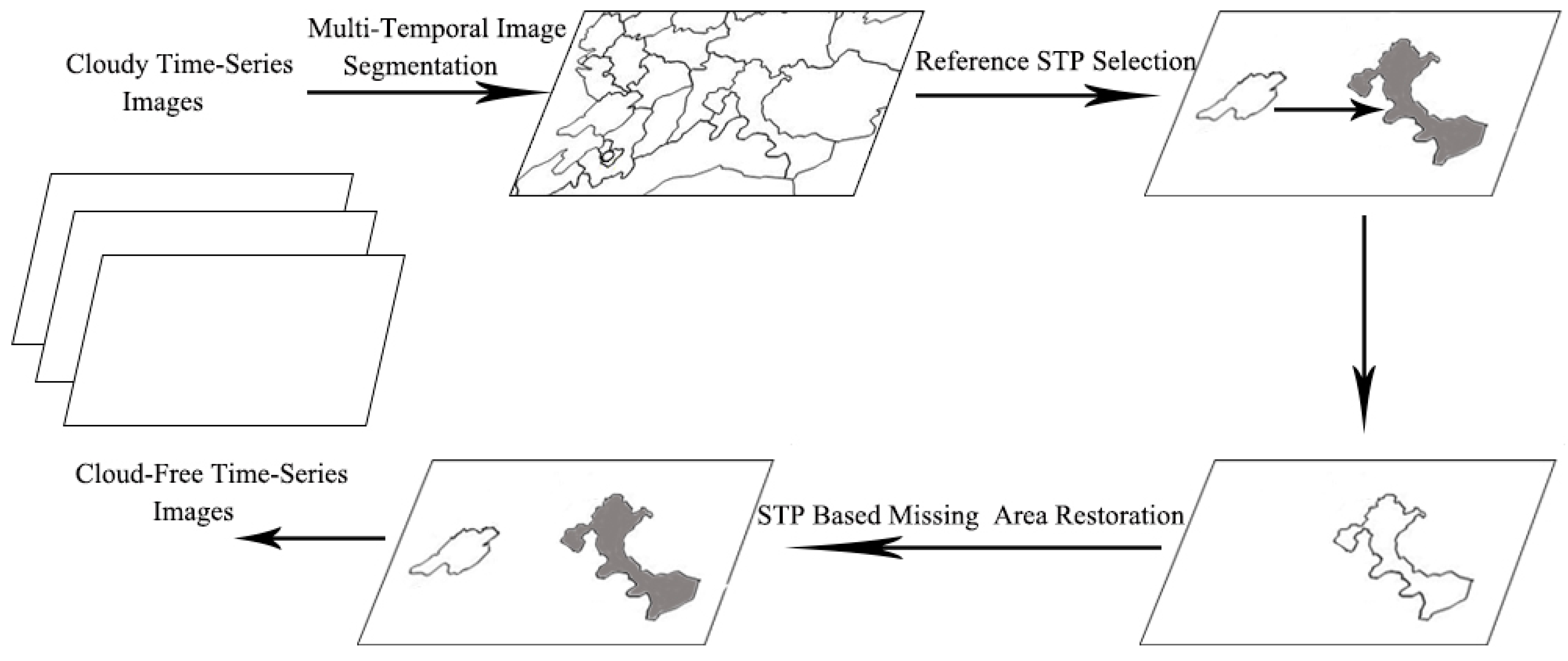
A multi-temporal image segmentation strategy, which incorporates spectral homogeneity and temporal evolution consistency, is utilized to extract the STP.

➢

The textural information from the clear temporal-adjacent image and the spectral information from the clear part of the same image are used to simultaneously reconstruct a missing STP, which will suppress the salt-and-pepper noise.

➢

The seam line will go through the actual edge defined by the STP, instead of the original seam line defined by the missing region and the valid region. As demonstrated by Soille [27], the actual edge between different STPs in the image will help conceal the false edge and obtain the seamless image.

The remainder of this paper is structured as follows. Section 2 introduces the reconstruction method of the missing area. Section 3 presents the experimental setting and the evaluation of the results. Section 4 discusses and analyzes the results of the method in this paper. Section 5 presents the conclusions of this paper.

2. Methods

In this paper, we propose a STP-based missing area reconstruction method for time-series images. Our method considers the STP with Missing Observation (STPMO) as a basic unit that searches for the reference STP and is to be reconstructed as a whole. At the same time, the textural information, denoted by the spatial arrangement of color or intensities for neighboring pixels [28], is extracted from the clear temporal-adjacent STP, and injected the missing observation. Through these methods, the reconstruction result not only avoids salt-and-pepper noise in the interior of the reconstructed STP, it also helps conceal the false edge between the reconstructed part and the remaining clear part.

For implementation, the proposed method includes three main procedures (as shown in Figure 1). (1) Multi-temporal image-based STP extraction: we divide the image into an ensemble of homogeneous patches using image segmentation with multi-temporal (most) cloud-free images. Since the segment obtained by our method has similar spectral and temporal evolution characteristics, we refer to the segmentation result as an STP. (2) Reference STP selection for the STPMO: we adopt a similar STP-based measurement to select the reference STP for the STPMO. (3) Missing STP reconstruction: we reconstruct the missing STP in the image according to the reference STP, and obtain cloud-free time-series images.

For the convenience of method description, we assume that we have obtained n scenes of an image of the same study area acquired on different dates. According to the date of acquisition, the n images can be expressed as I:

$$I=\{I^1,I^2,\dots ,I^n\}$$

(1)

Due to the CSS factor, some parts of the image are missing, which should be reconstructed by our method. First, we divide the region of every image in the time series into the valid part $\phi$ and the missing part $\varphi$ using an automatic mask method or a human-labeled method. For the image $I^m\in I$, the valid part and the missing part can be expressed as ${\phi }^m$ and ${\varphi }^m$, respectively, where ${\phi }^m$ and ${\varphi }^m$ satisfy:

$$I^m={\varphi }^m\cup {\phi }^m$$

(2)

$${\varphi }^m\cap {\phi }^m=\varnothing$$

(3)

where pixel $x_i^m\in {\varphi }^m$ is an invalid observation contaminated by CCS, i.e., a missing value, which should be estimated using the method proposed in this paper. By reconstructing the missing values of all of the images in the time series, we can obtain seamless time-series images.

2.1. Multi-Temporal Image Segmentation

Traditionally, image segmentation groups of adjacent pixels into a homogeneous region according to the similarities among the spectral characteristics of the pixels. The obtained homogeneous region forms the basic unit of analysis, which is generally referred to as a patch or segment. As a basic image-processing method, image segmentation has attracted increased attention, and a large number of image segmentation methods and improved versions have been proposed [29,30,31,32,33]. Mean shift segmentation has been extensively employed and achieved satisfactory performance in diverse applications. In mean shift segmentation, the cluster center constantly moves toward the density gradient ascending direction, which is referred to as drift, and therefore obtains the region of high density, and the pixels, which passed through during the process of searching the high-density regions, form a segment [32]. Numerous studies have addressed the principles and improvement of mean shift segmentation [33], which will not be repeated here.

The objective of the traditional image segmentation method is to split the image into an ensemble of homogenous regions, which is referred to as a segment, object, or patch. However, the pixels of a segment in our paper will require not only the same spectral characteristics but also similar temporal evolution; we denote them as STPs. To obtain the STPs, we adopt a multi-temporal image segmentation strategy similar to Dutrieux [31] and Desclée [34]. We selected multi-images from the time-series images to perform image segmentation. The selection of the images for segmentation considers two factors. (1) Proportion of valid pixels in the image: to obtain the image segmentation results for the entire study area, a cloud-free image in the entire study area is needed. (2) Date of the image acquisition: since vegetative land cover (such as forest and crops) has the distinct feature of temporal evolution, and selecting an image acquired at the temporal window (the best time(s) of image acquisition for vegetative land cover discrimination) will better differentiate the various STP types [35].

For convenience in processing, we select three scenes of images for segmentation. However, if we separately segment the three images, inconsistent segmentation results will likely be obtained for the various scenes. Thus, many small segmentation STPs can appear around the border of the segmentation results. Since vegetative information is primarily concentrated in the near-infrared band, the near-infrared band of three images is utilized to construct a new image; the color of the obtained image indicates the temporal evolution of the image, and the texture exhibits local contrast and similarity information. The new image is fed to segmentation, and we obtain the STP set P with m STPs, which can be expressed as follows:

$$P=\{P_1,P_2,\dots ,P_m\}$$

(4)

By multi-temporal image segmentation, the pixels within an STP will have not only similar spectral characteristics, but also similar temporal evolution. We calculate the mean ${\mu }_{P_{\mathrm{i}}}^{\mathrm{j}}$ and standard deviation ${\sigma }_{P_i}^{\mathrm{j}}$ of the grayscale value for STP $P_i\in P,i=1,2,\dots ,m$ for image $I^{\mathrm{j}}\in I$:

$${\mu }_{P_i}^j=\frac{1}{\left|P_i\right|}{\displaystyle \sum _{(\mathrm{r},\mathrm{c})\in P_i}{x}_{(\mathrm{r},\mathrm{c})}^j}$$

(5)

$${\sigma }_{Pi}^j=\sqrt{\frac{1}{\left|P_i\right|}{\displaystyle \sum _{(r,c)\in P_i}{(x_{(\mathrm{r},\mathrm{c})}^j-{\mu }_{P_i}^j)}^2}}$$

(6)

where $(r,c)\in P_{\mathrm{i}}$ represents a pixel with row $r$ and column $c$, which belongs to the STP of $P_{\mathrm{i}}$; $x_{(r,c)}^j$ denotes the grayscale value of a pixel with row $r$ and column $c$ on image $I^j$; and $\left|P_i\right|$ is the pixel number of the STP $P_{\mathrm{i}}$. On this basis, the mean and standard deviation grayscale value of the STP $P_{\mathrm{i}}$ are calculated for every image in $I$; the results form the mean vector ${\mu }_{P_{\mathrm{i}}}$ and the standard deviation vector ${\sigma }_{P_i}$, which can be expressed as:

$${\mu }_{P_i}=\{{\mu }_{P_i}^1,{\mu }_{P_i}^2,\dots ,{\mu }_{P_i}^n\}$$

(7)

$${\sigma }_{P_i}=\{{\sigma }_{P_i}^1,{\sigma }_{P_i}^2,\dots ,{\sigma }_{P_i}^n\}$$

(8)

The vector ${\mu }_{P_{\mathrm{i}}}$ depicts the temporal evolution of the mean grayscale value of the STP $P_{\mathrm{i}}$, and the vector ${\sigma }_{P_i}$ describes its variation magnitude.

2.2. Reference STP Selection for the STPMO

Assume that the data are missing in the region of STP $P_i\in P$ in image $I^{\mathrm{m}}\in I$ (i.e., $P_i\in {\varnothing }^m$), which is an STPMO, in other words, ${\mu }_{P_i}^m$ and ${\sigma }_{P_i}^m$ are unknown. For the convenience of description, we set ${\mu }_{P_i}^m$ and ${\sigma }_{P_i}^m$ to −1. Therefore, we should estimate ${\mu }_{P_i}^m$ and ${\sigma }_{P_i}^m$ using the reference STP $P_r$, whose mean (${\mu }_{P_r}^{\mathrm{m}}$) and standard deviation (${\sigma }_{P_r}^{\mathrm{m}}$) are known in the image $I^{\mathrm{m}}$. According to this analysis, the problem has been transformed to determine the reference STP.

The reference STP should have similar temporal-spectral features as the missing STP. The correlation coefficient describes the linear correlation between two variables. When it is applied to describe the similarity of the time-series spectral measurement (such as the grayscale value), the correlation coefficient indicates the reliability of using the reference variable to predict the variable with a missing observation. According to this analysis, we calculate the linear correlation coefficient $C(P_i,P_j)$ between STPs $P_{\mathrm{i}}$ and $P_{\mathrm{j}}$:

$$C(P_i,P_j)=\frac{{\displaystyle \sum _t(u_{P_i}^t-\mu ({\mu }_{P_i}))(u_{P_j}^t-\mu ({\mu }_{P_j}))}}{\sqrt{{\displaystyle \sum _t{(u_{P_i}^t-\mu ({\mu }_{P_i}))}^2}}\sqrt{{\displaystyle \sum _t{(u_{P_j}^t-\mu ({\mu }_{Pj}))}^2}}}$$

(9)

$$t=1,2,\dots ,n,{\mu }_{P_i}^t\ne -1\wedge {\mu }_{P_j}^t\ne -1$$

(10)

where ${\mu }_{P_i}^t$ and ${\mu }_{P_j}^t$ are the mean grayscale values for STPs $P_{\mathrm{i}}$ and $P_{\mathrm{j}}$ on image $I^{\mathrm{t}}\in I$, respectively, $u({\mu }_{P_i})$ and $\mu ({\mu }_{P_j})$ are the mean value of vector ${\mu }_{P_i}$ and ${\mu }_{P_j}$, respectively.

While calculating the correlation coefficient, we use only the valid value of ${\mu }_{P_i}^t$ and ${\mu }_{P_j}^t$ (i.e., ${\mu }_{P_i}^t\ne -1\wedge {\mu }_{P_j}^t\ne -1$, as indicated by Equation (10)). The dimension of the input vector for different STPs is inconsistent. Since the value of the correlation coefficient is a real number in the range of [–1, 1], for a situation that lacks one dimension, the fluctuation will not be excessive, but can reflect the linear correlation among the input remaining variables.

We use the $k$ STPs with the largest correlation coefficient $C(P_i,P_j)$ as the candidate reference STP $R(P_i)$ of STP $P_i$. However, the candidate reference STPs can only ensure that the reference STP and STPMO values have a similar temporal–spectral variation; their grayscale value distribution range may differ significantly. The standard deviation can quantitatively describe the grayscale values’ variation amplitude in an STP. The standard deviation similarity between two STPs $P_{\mathrm{i}}$ and $P_k$ can be described by the Euclidean distance $D(P_i,P_k)$, which can be calculated as:

$$D(P_i,P_k)=\sqrt{\frac{1}{n}{\displaystyle \sum _{t=1}^n{({\sigma }_{P_i}^t-{\sigma }_{p_k}^t)}^2}}$$

(11)

where STP $P_k\in R(P_i)$. We consider the STP with the smallest Euclidean distance in $R(P_i)$ as the reference STP of STP P_i and denote it as $P_r$:

$$P_r=\underset{P_k\in R(P_i)}{\arg \min }(D(P_i,P_k))$$

(12)

2.3. Missing Value Estimation for STPMO

Missing value estimation for STPMO includes two steps: (I) estimation of the mean and standard deviation of the STPMO, and (II) textural information injection. The implementation details are introduced as follows:

(I) Estimation of the mean and standard deviation of the STPMO

According to the analysis, the mean vector of the missing STP $P_i$ and the reference STP $P_r$ has a high linear correlation. Therefore, a linear regression model is used to describe their relationship. The linear regression coefficient $<k_u,b_u>$ can be obtained by least squares regression with the remaining valid observations in the time series. The estimated mean value for the STP P_i, ${\widehat{u}}_{P_i}^m$, can be expressed as:

$${\widehat{u}}_{P_i}^m=k_u*{\mu }_{\mathrm{Pr}}^m+b_u$$

(13)

Since the reference STP is selected using the minimum Euclidean distance of the standard deviation, we directly obtain the estimation of value ${\widehat{\sigma }}_{P_i}^m$ using ${\sigma }_{P_r}^m$:

$${\widehat{\sigma }}_{P_i}^m={\sigma }_{P_r}^m$$

(14)

(II) Textural information injection

To recover the rich texture of the STP $P_{\mathrm{i}}$ in image $I^{\mathrm{m}}$, we “inject” the rich textural information exhibit in the corresponding region of image $I^l$ into the missing part of image $I^{\mathrm{m}}$. First, we should select a reference image to extract the textual information. The determination of the temporal-adjacent image $I^l$ for image $I^{\mathrm{m}}$ depends on two conditions: (1) the region of STP $P_{\mathrm{i}}$ in the image in image $I^l$ is valid; and (2) based on satisfying condition (1), we select the acquisition date of two images as close as possible—i.e., the temporal interval between $I^{\mathrm{m}}$ and $I^l$ is the smallest.

The textural information from the temporal-adjacent image will be injected to the STPMO under the restrictive condition of the estimated mean (${\widehat{u}}_{P_i}^m$) and standard deviation (${\widehat{\sigma }}_{P_i}^m$). For pixel $x_{P_{\mathrm{i}}}^{\mathrm{m}}$, whose value is missing, the estimation value ${\widehat{x}}_{P_i}^m$ can be calculated as:

$${\widehat{x}}_{P_i}^m=\frac{{\widehat{\sigma }}_{P_i}^m}{{\sigma }_{P_i}^l}{x}_{P_i}^l+({\widehat{\mu }}_{P_i}^m-\frac{{\widehat{\sigma }}_{P_i}^m}{{\sigma }_{Pi}^l}{\mu }_{Pi}^l)$$

(15)

where ${\mu }_{P_i}^l$ and ${\sigma }_{P_i}^l$ are the mean and standard deviation, respectively, of the grayscale value in the STP P_i on the image $I^l$; ${\widehat{u}}_{P_i}^m$ and ${\widehat{\sigma }}_{P_i}^m$ are the estimated mean and standard deviation, respectively, of the grayscale value. As shown in Equation (15), the grayscale of the reconstructed STPMO will obey a distribution, where the mean is ${\widehat{u}}_{P_i}^m$ and the standard deviation is ${\widehat{\sigma }}_{P_i}^m$. From the above procedure, we can see that neighboring pixels in the reconstructed area will have similar reconstruction accuracy, which helps preserve the spatial arrangement color or intensity information; removing the inconsistent pixel will suppress the salt-and-pepper noise effect.

For the STP $P_{\mathrm{i}}$ in the image $I^{\mathrm{m}}$, the missing part may be partial or complete. For cases in which only part of the STP data is missing, if the missing ratio exceeds r, we treat the valid pixels as the missing pixel, and reconstruct them using the method. If the missing ratio is smaller than r, then we use the remaining clear part (denoted as $\phi (P_i)$) to construct the missing part (denoted as $\varphi (P_i)$). The setting of r should take into consideration that the valid part must provide enough information to reconstruct the missing part. By the trial and error method, we find that r set 0.5 is a proper value to balance the valid pixel preservation and missing pixel restoration. Then, we calculate the mean and standard deviation of the grayscale value for the valid region of P_i ($\phi (P_i)$) on the image $I^{\mathrm{m}}$, which can be expressed as ${\mu }_{\phi (P_i)}^m$ and ${\sigma }_{\phi (P_i)}^m$, respectively. The mean and standard deviation of the grayscale value on the image $I^l$ are ${\mu }_{\phi (P_i)}^l$ and ${\sigma }_{\phi (P_i)}^l$, respectively. For the missing value, we adopt the following equation for the reconstruction:

$${\widehat{x}}_{\varphi (P_i)}^m=\frac{{\sigma }_{\phi (P_i)}^m}{{\sigma }_{\phi (P_i)}^l}{x}_{\varphi (P_i)}^l+({\mu }_{\phi (P_i)}^m-\frac{{\sigma }_{\phi (P_i)}^m}{{\sigma }_{\phi (P_i)}^l}{\mu }_{\phi (P_i)}^l)$$

(16)

Since CCS can induce a data missing problem for any date of time-series images, the missing observation number in the time series is not consistent among different STPs. Generally, the smaller the missing number in the time series of the STP, the stronger the ability of the correlation coefficient to describe the linear correlation, which increases the probability of selection of the proper reference STP. Therefore, we sort the STP according to the missing data number in descending order, and sequentially reconstruct the missing STP. For example, we reconstruct the STPs with one missing observation using the free STP. The STPs with two missing observations are reconstructed using the free STP and the previously reconstructed STP with one missing. Then, we repeat this process until the STPs with missing observations have been reconstructed, and can thus obtain an entire seamless time series of images.

According to the implementation procedures, the mean and standard deviation are estimated using the reference STP in the same image, which guarantees that the reconstructed STP is consistent with the remaining clear part. Since the texture of the missing STP is injected according to the temporal-adjacent images and normalized by the estimated mean and standard deviation, the pixels in the missing STP will have similar reconstruction accuracy. The seam line of the reconstructed part and remaining part has been shifted to the actual edge between different STPs, which can help conceal the false edge.

3. Experimental

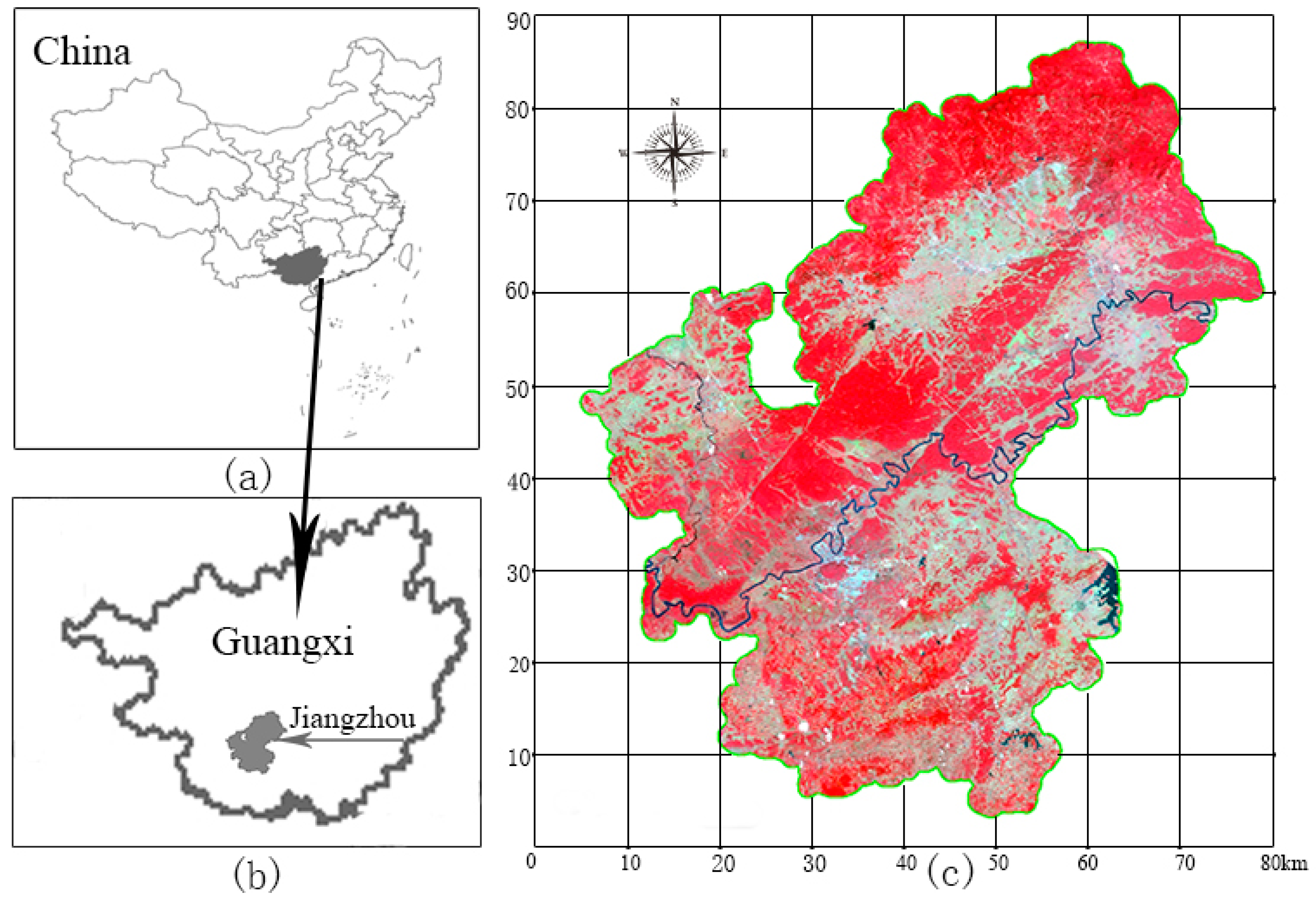
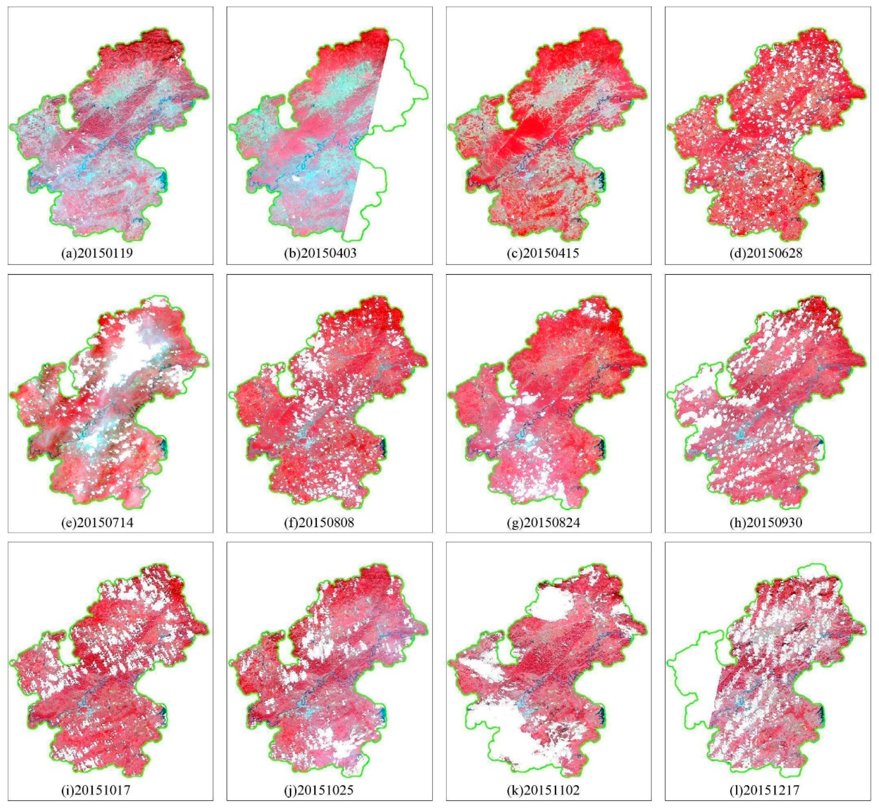
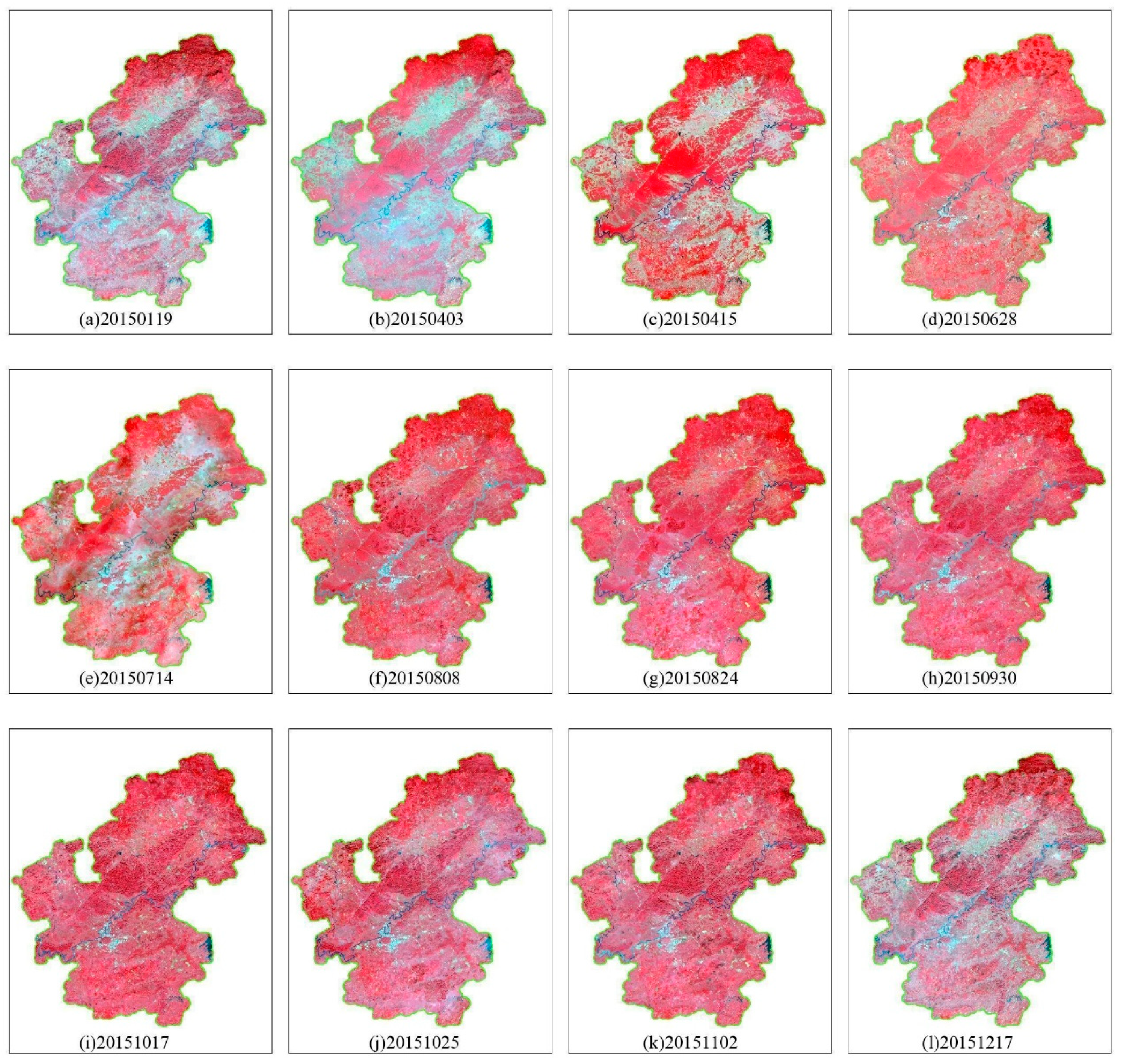
3.1. Study Area and Data

The study area is located in the Jiangzhou District of Chongzuo City in the Guangxi Zhuang Autonomous Region in China, which covers an area of 2901 km², as shown in Figure 2. The terrain in the study area is high in the northeast and low in the southwest; the Zuojiang River passes through the middle of the Jiangzhou District. Farmland is the dominant land-use type in the study area. The study area has an abundance of water and heat and occurred in the same period, which renders it suitable for sugarcane growth [36]. Sugarcane is extensively grown on the flat ground or gentle slopes. Thus, this region is the main sugarcane-producing area in China, and sugarcane is the main local economic crop [37]. Due to decentralized cultivation by individual farmers, the sowing, cutting, and harvesting of sugarcane rely on manpower, which increases the planting costs. Centralized farmland planting via land-use right transfer has importance for improving the economic efficiency and increasing the income of the farmers. A spatial-explicit crop map derived from time-series remote sensing images forms the basis for land suitability assessment and improves agricultural gain [38]. Jiangzhou is in the subtropical zone, which is characterized by cloudy and rainy weather [36]; this hinders the acquisition of cloud-free images. The complete exploitation of partially missing images will lay the foundation for all passive remote sensing applications.

To test the proposed method, we identified 16 scenes of images obtained in 2015 by the wide field view (WFV) sensor onboard the Chinese GaoFen1 satellite, which has a spatial resolution of 16 m and four spectral channels: near-infrared, red, green, and blue. The details of the sensor characteristics are listed in

Table 1. Characteristic of the wide field view sensor onboard Chinese GaoFen1 (GF1). NIR: near-infrared.

Spectral Band	Name	Band Range (µm)	Spatial Resolution (m)	Field Width (km)	Revisit Time (Day)
B1	blue	0.45–0.52	16	800	2
B2	green	0.52–0.59
B3	red	0.63–0.69
B4	NIR	0.77–0.89

. The images are processed via Image Processing Machine (IPM) software (developed by ImageSky) for fine geometric correction. We exclude the images whose geometric errors after fine geometric correction exceeded one pixel; 12 scenes of an image remain. The metadata are shown in

Table 2. Metadata of time-series images. WFV: wide field view.

No.	Sensor	Image Acquisition Date	Missing Area Percent
1	WFV2	19 January 2015	1.2
2	WFV2	3 April 2015	20
3	WFV1	15 April 2015	0.1
4	WFV2	28 June 2015	16.2
5	WFV1	14 July 2015	21.2
6	WFV2	8 August 2015	16.3
7	WFV1	24 August 2015	9.9
8	WFV1	30 September 2015	24.5
9	WFV4	17 October 2015	20.8
10	WFV2	25 October 2015	16.7
11	WFV1	2 November 2015	31.6
12	WFV2	17 December 2015	38.4

. The CCS-masked images, which are clipped by the boundary of the study area, are shown in Figure 3. Transforming the original grayscale value to a physical signal, such as top-of-atmosphere (TOA), may increase the comparability among different images and improve the reconstruction accuracy. Due to the lack of radiometric correction parameters during the image distribution, we directly employ the grayscale value. The initial missing area mask is obtained by automatic processing and modified by human interpretation to ensure an accurate CCS mask. The missing percentage of different scenes of the image is diverse, and each pixel has approximately 8.5 valid observations.

We selected three scenes of images with acquisition dates of 19 January, 15 April, and 24 August for image segmentation. These three multi-temporal images were selected because the differentiation of the various vegetation in these images was better, and the missing proportion on the image was relatively small (smaller than 10%). The missing values in the three images were directly filled with the corresponding pixels in the temporal-adjacent pixel for multi-temporal image segmentation. We employ the default spectral and spatial bandwidth (i.e., 6.5 and 7, respectively) for image segmentation [39]. Under the guidance of the reference [39] and visual inspection of the segmentation result, we set the segmentation scale to 100, which indicates that the lowest pixel number of a STP approaches 100. We obtain 39,116 STPs. According to the statistics, the lowest number of valid observations in the time series in different STPs is six. We employ the STP as the basic unit to reconstruct the missing values and obtain seamless time-series images.

3.2. Experimental Method and Evaluation Method

The profile-based interpolator (PBL) method selects the reference curve based on the morphological similarity of the time-series curve and estimates missing values [20]. The principal of the PBL method is similar to that of our method; thus, we select it as the contrasting method. The difference is that the contrasting method reconstructs the missing area pixel-by-pixel, whereas our method uses the STP as the basic unit for the missing area reconstruction. To obtain the most accurate estimation of the missing value, the contrasting method searches for the reference pixel in the entire image.

We select four types of STPs (i.e., farmland, forest, city, and water) without missing time-series observations, whose 12 observations are valid in the time-series images. According to the ratio of the STP type in the study area, the number of STPs of each STP type is 20, 10, 10, and 5, respectively. We generated the missing values in these STPs and reconstructed them using our method and the contrasting method. The results are compared with the actual value to evaluate the accuracy of the two methods.

To quantitatively evaluate the accuracy of the methods, we calculated the error $e_i$ of pixel i in the reconstruction region as follows:

$$e_i=|x_i-{\widehat{x}}_i|$$

(17)

where $x_i$ is the true value, i.e., the simulated missing value, and ${\widehat{x}}_i$ is the estimated value by our method or the contrasting method. The smaller the value of e, the higher the accuracy.

For the total reconstruction accuracy of the missing region, we adopted the root mean square error (RMSE), standard deviation of the error (SDE), and correlation coefficient (CC) for quantitative evaluation. The RMSE indicates the deviation between the actual observation and the reconstructed result; SDE represents the concentration of the error distribution; and CC depicts the textural similarity between the actual observation and the reconstructed result. The calculation method is expressed as:

$$RMSE=\sqrt{\frac{1}{\left|\varphi \right|}{\displaystyle \sum _{i\in \varphi }{(e_i)}^2}}$$

(18)

$$SDE=\sqrt{\frac{1}{\left|\varphi \right|}{{\displaystyle \sum _{i\in \varphi }(e_i-u(e))}}^2}$$

(19)

$$CC=\frac{|\varphi |{\displaystyle \sum _{i\in \varphi }{x}_i{\stackrel{⌢}{x}}_i}-{\displaystyle \sum _{i\in \varphi }{x}_i}{\displaystyle \sum _{i\in \varphi }{\stackrel{⌢}{x}}_i}}{\sqrt{|\varphi |{\displaystyle \sum _{i\in \varphi }{(x_i)}^2}-({\displaystyle \sum _{i\in \varphi }{x}_i{)}^2}}\sqrt{|\varphi |{\displaystyle \sum _{i\in \varphi }{({\stackrel{⌢}{x}}_i)}^2}-({\displaystyle \sum _{i\in \varphi }{\stackrel{⌢}{x}}_i{)}^2}}}$$

(20)

where $\varphi$ is the missing area, and $\left|\varphi \right|$ is the number of pixels in the missing area.

3.3. Experimental Results

Figure 4 shows the reconstruction results of our method. Viewing all of the images as a whole, we can discover the evolution process of the study area, which demonstrates that the capacity of our reconstructed data can describe the landscape dynamics. Figure 5 provides an original image (Figure 5a), our result (Figure 5b), and the contracting result (Figure 5c). By magnifying the reconstruction area (as shown in Figure 5d–f), we observe that (1) the reconstructed region of our method (Figure 5e) can restore the textural features and provide sufficient information, whereas the contrasting method (Figure 5f) is substantially influenced by salt-and-pepper noise, which conceals the local spectral contract of the land surface; and (2) the reconstructed part is consistent with the clear part of the image without a distinct false edge, which indicates that the reconstructed part and clear part blend well. In general, our method can maintain the local texture information and the reconstructed part exhibit better spectral consistency with the remaining clear part.

Figure 6 shows the reconstruction results of our method and the contrasting method for the four typical simulated missing STPs (i.e., farmland, forest, water, and cities). We observe that the reconstruction results of our method provide rich texture information, and the consistence with the surrounding clear pixels is better than that of the contrasting method. The contrasting method shows some salt-and-pepper noise and a mosaic phenomenon. The fourth and fifth columns of Figure 6 show the error distribution for the NIR band of our method and the contrasting method. The error distribution of our method is compact, whereas the error distribution range of the contrasting method is wide. The sixth column of Figure 6 reveals that the error of our method is smaller than that of the contrasting method in most cases. We conclude that our method outperforms the contrasting method in terms of accuracy.

Table 3. Statistical result of Our MethoD (OMD) and the Contrasting MethoD (CMD). CC: correlation coefficient, RMSE: root mean square error, SDE: standard deviation of the error.

Band	Method	Farmland			Forest			Water			City
		RMSE	SDE	CC	RMSE	SDE	CC	RMSE	SDE	CC	RMSE	SDE	CC
NIR	OMD	20.24	60.24	0.95	32.99	46.84	0.94	40.29	36.09	0.84	17.74	30.33	0.88
	CMD	33.35	72.61	0.91	54.58	55.15	0.87	26.85	45.74	0.81	26.43	32.29	0.80
Red	OMD	20.85	45.29	0.86	21.34	18.48	0.85	40.34	16.31	0.72	13.26	36.56	0.97
	CMD	45.29	45.19	0.87	26.75	24.01	0.67	43.61	16.53	0.83	18.84	40.66	0.88
Green	OMD	16.81	22.9	0.69	8.70	7.39	0.58	10.5	11.8	0.61	9.90	9.13	0.94
	CMD	12.9	23.39	0.68	8.29	16.06	0.48	4.78	11.78	0.78	9.10	10.22	0.86

illustrates the statistical results of our method and the contrasting method. The results indicate that the RMSE of our method is smaller than or comparable to that of the contrasting method, which demonstrates that our method can achieve greater accuracy. Note that the RMSE is similar in different bands, which indicates that our method can preserve the color fidelity. The SDE obtained by our method is smaller than that of the contrasting method, which indicates that the errors are concentrated in a small range. The concentrated error distribution will suppress the salt-and-pepper effect in the reconstructed area. The CC is higher in our result in most cases, which indicates that the reconstructed STP is linearly correlated with the actual STP, and that the textural information is more authentic.

Also, from Figure 6 and Table 3, some interesting phenomena can be observed. (1) Our method obtains lower accuracy for some pixels. This phenomenon can be attributed to our method reconstructing the STPMO as a whole, whereas the pixel-by-pixel selection may select a more similar pixel, thus making the reconstructed error become smaller. On the other hand, the pixel-by-pixel reference selection may induce an overfitting problem and have a low accuracy, but STP-based processing will operate in a robust way. (2) The error distribution (SDE) of our method outperforms that of the contrasting method, whereas the RMSE of our method is larger, such as the water of blue band (in Table 3). The temporal evolution of water cannot be well-defined, which may induce that we cannot find a similar STP with type of water for the STPMO, but the pixel-by-pixel selection can find more proper pixels and yield better accuracy. (3) The performance gain is smaller (or even performance loss) in the green and red bands between our method and the contrasting method. This can be attributed to the multi-temporal image segmentation adopting only the NIR band, which loses information that is present in the green and red bands to extract the STPs.

4. Discussion

4.1. Factors that Influence the Accuracy of the Algorithm

The STP is the basic unit for missing region reconstruction, and the spectral homogeneity and temporal variation consistency of the STP are important factors that determine the accuracy obtained by our method. The spectral homogeneity and temporal variation consistency of the STP are primarily exhibited as the STP size and the grayscale value distribution acquired on various dates. The size of the STP primarily depends on the selected segmentation scale. The size of the STP in this paper is 100. Figure 7a shows the distribution of the pixel numbers for the STPs. In particular, the size of 80% of the STPs is less than 400 pixels. Figure 7b shows the standard deviation of the grayscale value of the STP in the NIR band and its variation with time. A black point indicates the mean of the grayscale of an STP, and the red line represents the mean and standard deviation of all of the STPs. The distribution of the standard deviation for various STPs is relatively small in all of the images, which indicates that the grayscale characteristics of the STPs have satisfactory temporal evolution consistency. These results indicate that the multi-temporal image segmentation method that is utilized in this paper can obtain segmentation results with spectral homogeneity and temporal evolution consistency, which provide a firm basis for the construction of missing time-series data. Note that the distribution of the grayscale value for different STPs of the image obtained on 28 June 2015 exhibits a larger range; this is due to the deficiency from our use of the original grayscale value instead of a physical signal, which decreases the comparability among different images.

The underlying land-cover type, missing dates in the time series, and missing numbers are important factors that affect the accuracy of the algorithm. We calculate the mean RMSE for all of the simulated STPs with different types for the NIR band; the results are shown in Figure 8. We observe the following results:

➢

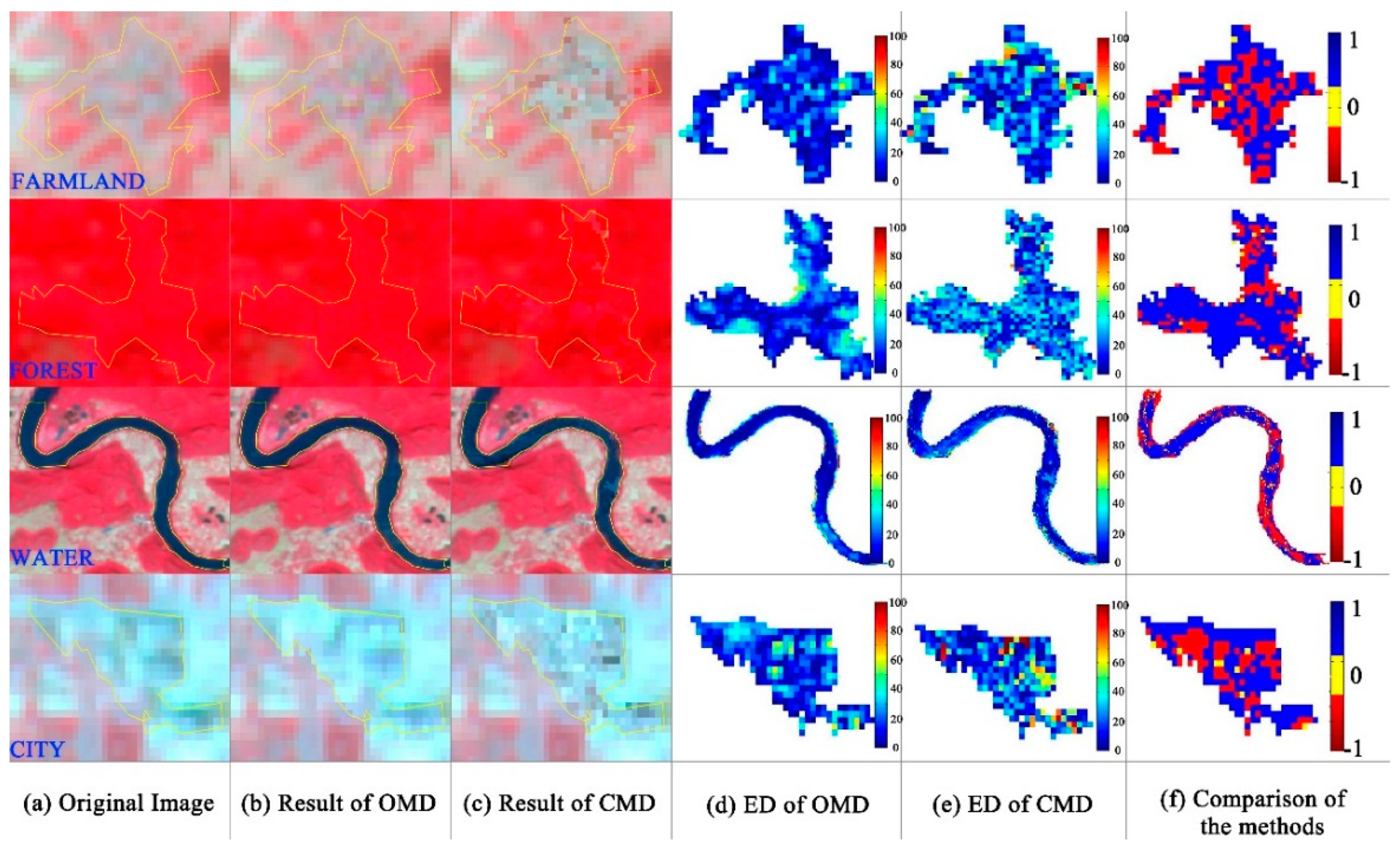
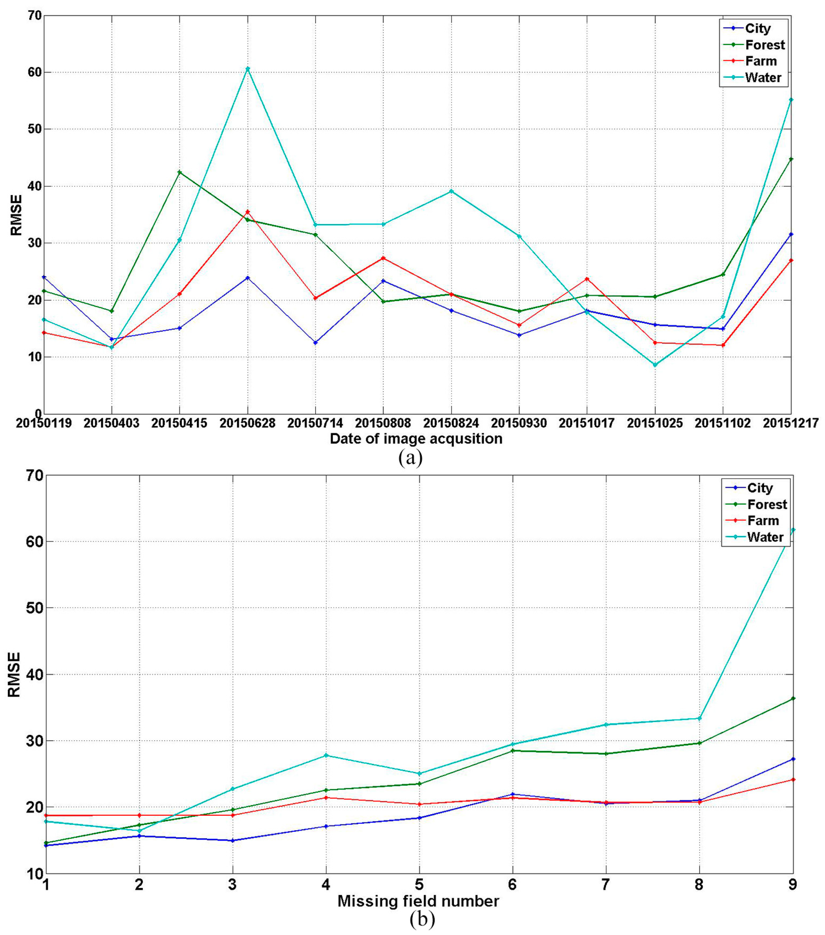
For different missing STP types. Figure 8a shows the RMSE with one missing time for four types of STPs (i.e., farmland, forest, city, and water). As expected, the higher reconstruction accuracy is obtained for the city, and lower reconstruction accuracy is obtained for forest, farmland, and the lowest is obtained for water. The spectral variation among the cities is relatively slow, whereas the forest and farmland exhibit relatively high temporal variation and are difficult to reconstruct. The estimation error of a water body is the largest, which is primarily attributed to the water being susceptible to sediment charge and chlorophyll content, which does not have a well-defined evolution process.

➢

For the missing date of the images. Figure 8a shows the simulation reconstruction accuracy of the corresponding data. The influence of the growth period of vegetation (forest and farmland) is large, and the influence of the stable time is small. The influence on accuracy for cities is small due to their small changes in the radiation characteristics.

➢

For the missing number in the time series. Figure 8b shows the variation of RMSE with an increasing missing number. The RMSE value generally increases as the number of missing observations increases; thus, the reconstruction accuracy decreases. Since the method in this paper selects the entire STP as the reference STP, when the reference STP of the missing STP does not change, the influence on the accuracy of the reconstruction results is small. However, when the selected reference STP changes, the accuracy exhibits a steep decrease.

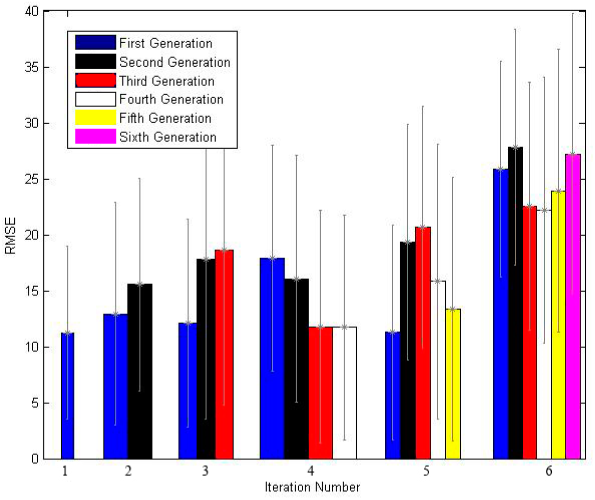
4.2. Error Propagation of the Early Reconstructed STP

Our method sorts STPs according to the missing observation number in the time series in ascending order and sequentially reconstructs the missing area. When we use the early reconstructed STP for the late missing STP reconstruction, error propagation or accumulation may occur. To quantitatively evaluate the error propagations, we perform an experiment to simulate the error propagation process. Assume that STP(B) is a STPMO and that STP(A) has been selected as the reference STP, and is utilized to reconstruct STP(B). We obtain the reconstructed result, which is denoted as STP(B1), i.e., iteration 1. For anther STP, which is denoted as STP(C) and whose reference STP is STP(B), because the STP(B) has two copies, i.e., the actual STP(B) and reconstructed result STP(B1), they can be applied to the reconstruction of STP(C), respectively. Therefore, we can obtain two reconstructed results STP(C1) and STP(C2), i.e., iteration 2. We can compare the reconstructed results STP(C1) and STP(C2) with STP(C) to evaluate the error propagation problem. For simplicity, we refer to the obtained result that was reconstructed with the actual observation as the first-generation result, and refer to the result reconstructed with the first-generation result as the second-generation result. Similarly, we can define the third-generation result, the fourth-generation result, and the remaining results.

We simulate the missing area in the nearly cloud-free image (image acquired on 15 April 2015) with six iterations. Ten simulated STPs have been selected. The mean and standard deviation of the RMSE calculated using the simulated STPMO are illustrated in Figure 9. The result demonstrates that (1) the RMSE variation between different generations is small. This finding can be explained as follows: the mean and standard deviation of the missing observations are estimated using the remaining clear observations in the time series by linear regression. One observation value variation (caused by the early reconstructed STP) does not significantly change the estimated value; (2) the RMSE of a subsequent generation is smaller than that of the earlier generation. This finding can be attributed to the missing value, which has been previously reconstructed and has a larger error. The early reconstruction is similar to removing an observation with a large error. As a result, the late reconstruction can yield a smaller RMSE. The result demonstrates that the utilization of the early reconstructed STPs does not produce a monotone increasing error, which demonstrates that this strategy can serve as an effective method for enriching the potential reference STPs and improving the reconstruction accuracy.

5. Conclusions

In this paper, we propose an STP-based missing area reconstruction method for a time-series image. The reconstruction results are characterized by rich texture information (without salt-and-pepper noise) and are consistent with the original image (without a false edge). Since the missing area is constructed STP by STP, which considerably decreases the search space for reference STP, the computational efficiency is substantially improved compared with pixel-by-pixel selection. Our method can complete the processing in hours, but the contrasting method will complete it in days. The STP represents different land covers with similar spectral characteristics and temporal evolution, and the actual edges between different STPs help conceal the false edge induced by the error between the reconstructed part and the remaining clear part.

Although many factors, such as the SLC-OFF for ETM+ onboard Landsat 7, may cause missing information in remote sensing images, the CCS is the most common factor. For convenience of description, we employ CCS-induced information about the missing area to represent the missing information caused by all of the factors. Our method can also be directly applied for missing area reconstruction induced by other factors.

However, this paper has some drawbacks to be solved in future studies. (1) Numerous factors, such as the missing observation number in the time series and the missing land-cover type, affect the accuracy of our method, which may cause uncertainty in the reconstruction results. (2) The direct utilization of a grayscale value may produce additional noise to the reconstructed result. (3) The STPs were obtained by multi-temporal image segmentation using only the NIR band and three scenes of images selected for conducting multi-temporal image segmentation, which may omit some information contained in the remaining bands or images. An improved method may adopt an image segmentation method that can simultaneously handle additional bands and process incomplete data.

References

- Kaufman, Y. The effect of subpixel clouds on remote sensing. Int. J. Remote Sens. 1987, 8, 839–857. [Google Scholar] [CrossRef]
- Zhang, Y.; Guindon, B.; Cihlar, J. An image transform to characterize and compensate for spatial variations in thin cloud contamination of Landsat images. Remote Sens. Environ. 2002, 82, 173–187. [Google Scholar] [CrossRef]
- Cai, Y.; Guan, K.; Peng, J.; Wang, S.; Seifert, C.; Wardlow, B.; Li, Z. A high-performance and in-season classification system of field-level crop types using time-series Landsat data and a machine learning approach. Remote Sens. Environ. 2018, 210, 35–47. [Google Scholar] [CrossRef]
- Huang, C.; Goward, S.N.; Masek, J.G.; Thomas, N.; Zhu, Z.; Vogelmann, J.E. An automated approach for reconstructing recent forest disturbance history using dense Landsat time series stacks. Remote Sens. Environ. 2010, 114, 183–198. [Google Scholar] [CrossRef]
- Dara, A.; Baumann, M.; Kuemmerle, T.; Pflugmacher, D.; Rabe, A.; Griffiths, P.; Hölzel, N.; Kamp, J.; Freitag, M.; Hostert, P. Mapping the timing of cropland abandonment and recultivation in northern Kazakhstan using annual Landsat time series. Remote Sens. Environ. 2018, 213, 49–60. [Google Scholar] [CrossRef]
- Yan, L.; Roy, D.P. Improved time series land cover classification by missing-observation-adaptive nonlinear dimensionality reduction. Remote Sens. Environ. 2015, 158, 478–491. [Google Scholar] [CrossRef]
- Holben, B.N. Characteristics of maximum-value composite images from temporal AVHRR data. Int. J. Remote Sens. 1986, 7, 1417–1434. [Google Scholar] [CrossRef] [Green Version]
- Brooks, E.B.; Thomas, V.A.; Wynne, R.H.; Coulston, J.W. Fitting the multitemporal curve: A fourier series approach to the missing data problem in remote sensing analysis. IEEE Trans. Geosci. Remote Sens. 2012, 50, 3340–3353. [Google Scholar] [CrossRef]
- Vuolo, F.; Ng, W.-T.; Atzberger, C. Smoothing and gap-filling of high resolution multi-spectral time series: Example of Landsat data. Int. J. Appl. Earth Obs. Geoinf. 2017, 57, 202–213. [Google Scholar] [CrossRef]
- Maxwell, S.K.; Schmidt, G.L.; Storey, J.C. A multi-scale segmentation approach to filling gaps in Landsat ETM+ SLC-off images. Int. J. Remote Sens. 2007, 28, 5339–5356. [Google Scholar] [CrossRef]
- Zhang, C.; Li, W.; Travis, D.J. Restoration of clouded pixels in multispectral remotely sensed imagery with cokriging. Int. J. Remote Sens. 2009, 30, 2173–2195. [Google Scholar] [CrossRef]
- Maalouf, A.; Carre, P.; Augereau, B.; Fernandez-Maloigne, C. A Bandelet-Based inpainting technique for clouds removal from remotely sensed images. IEEE Trans. Geosci. Remote Sens. 2009, 47, 2363–2371. [Google Scholar] [CrossRef]
- Helmer, E.H.; Ruefenacht, B. Cloud-free satellite image mosaics with regression trees and histrogram matching. Photogramm. Eng. Remote Sens. 2005, 71, 1079–1089. [Google Scholar] [CrossRef]
- Helmer, E.H.; Ruefenacht, B. A comparison of radiometric normalization methods when filling cloud gaps in Landsat imagery. Can. J. Remote Sens. 2007, 33, 325–340. [Google Scholar] [CrossRef]
- Melgani, F. Contextual reconstruction of cloud-contaminated multitemporal multispectral images. IEEE Trans. Geosci. Remote Sens. 2006, 44, 442–455. [Google Scholar] [CrossRef]
- Lin, C.; Tsai, P.; Lai, K.; Chen, J. Cloud removal from multitemporal satellite images using information cloning. IEEE Trans. Geosci. Remote Sens. 2013, 51, 232–241. [Google Scholar] [CrossRef]
- Lorenzi, L.; Melgani, F.; Mercier, G. Missing-Area reconstruction in multispectral images under a compressive sensing perspective. IEEE Trans. Geosci. Remote Sens. 2013, 51, 3998–4008. [Google Scholar] [CrossRef]
- Zhu, X.; Gao, F.; Liu, D.; Chen, J. A modified neighborhood similar pixel interpolator approach for removing thick clouds in Landsat images. IEEE Geosci. Remote Sens. Lett. 2012, 9, 521–525. [Google Scholar] [CrossRef]
- Cheng, Q.; Shen, H.; Zhang, L.; Yuan, Q.; Zeng, C. Cloud removal for remotely sensed images by similar pixel replacement guided with a spatio-temporal MRF model. ISPRS J. Photogramm. Remote Sens. 2014, 92, 54–68. [Google Scholar] [CrossRef]
- Malambo, L.; Heatwole, C.D. A multitemporal profile-based interpolation method for gap filling nonstationary data. IEEE Trans. Geosci. Remote Sens. 2016, 54, 252–261. [Google Scholar] [CrossRef]
- Yan, L.; Roy, D.P. Large-area gap filling of Landsat reflectance time series by spectral-angle-mapper based spatio-temporal similarity (SAMSTS). Remote Sens. 2018, 10, 609. [Google Scholar] [CrossRef]
- Gao, G.; Gu, Y. Multitemporal Landsat missing data recovery based on tempo-spectral angle model. IEEE Trans. Geosci. Remote Sens. 2017, 55, 3656–3668. [Google Scholar] [CrossRef]
- Chen, B.; Huang, B.; Chen, L.; Xu, B. Spatially and temporally weighted regression: A novel method to produce continuous cloud-free landsat imagery. IEEE Trans. Geosci. Remote Sens. 2017, 55, 27–37. [Google Scholar] [CrossRef]
- Pouliot, D.; Latifovic, R. Reconstruction of Landsat time series in the presence of irregular and sparse observations: Development and assessment in north-eastern Alberta, Canada. Remote Sens. Environ. 2018, 204, 979–996. [Google Scholar] [CrossRef]
- Blaschke, T. Object based image analysis for remote sensing. ISPRS J. Photogramm. Remote Sens. 2010, 65, 2–16. [Google Scholar] [CrossRef]
- Zomet, A.; Levin, A.; Peleg, S.; Weiss, Y. Seamless image stitching by minimizing false edges. IEEE Trans. Image Process. 2006, 15, 969–977. [Google Scholar] [CrossRef] [PubMed] [Green Version]
- Soille, P. Morphological image compositing. IEEE Trans. Pattern Anal. Mach. Intell. 2006, 28, 673–683. [Google Scholar] [CrossRef] [PubMed]
- Shapiro, L.G.; Stockman, G.C. Computer Vision; Prentice-Hall: Upper Saddle River, NJ, USA, 2001. [Google Scholar]
- Tilton, J.C.; Tarabalka, Y.; Montesano, P.M.; Gofman, E. Best merge region-growing segmentation with integrated nonadjacent region object aggregation. IEEE Trans. Geosci. Remote Sens. 2012, 50, 4454–4467. [Google Scholar] [CrossRef]
- Li, D.; Zhang, G.; Wu, Z.; Yi, L. An edge embedded marker-based watershed algorithm for high spatial resolution remote sensing image segmentation. IEEE Trans. Image Process. 2010, 19, 2781–2787. [Google Scholar] [PubMed]
- Dutrieux, L.P.; Jakovac, C.C.; Latifah, S.H.; Kooistra, L. Reconstructing land use history from Landsat time-series: Case study of a swidden agriculture system in Brazil. Int. J. Appl. Earth Obs. Geoinf. 2016, 47, 112–124. [Google Scholar] [CrossRef]
- Comaniciu, D.; Meer, P. Mean shift: A robust approach toward feature space analysis. IEEE Trans. Pattern Anal. Mach. Intell. 2002, 24, 603–619. [Google Scholar] [CrossRef]
- Michel, J.; Youssefi, D.; Grizonnet, M. Stable mean-shift algorithm and its application to the segmentation of arbitrarily large remote sensing images. IEEE Trans. Geosci. Remote Sens. 2015, 53, 952–964. [Google Scholar] [CrossRef]
- Desclée, B.; Bogaert, P.; Defourny, P. Forest change detection by statistical object-based method. Remote Sens. Environ. 2006, 102, 1–11. [Google Scholar] [CrossRef]
- Van Niel, T.G.; Mcvicar, T.R. Determining temporal windows for crop discrimination with remote sensing: A case study in south-eastern Australia. Comput. Electron. Agric. 2004, 45, 91–108. [Google Scholar] [CrossRef]
- Leng, W.; Liang, Y.; Lu, B. Climate suitability analysis for sugarcane planting in Chongzuo city. Agric. Environ. Resour. 2015, 3, 229–231. (In Chinese) [Google Scholar]
- Wang, X.; Ruan, H.; Huang, Z. Analysis on potential productivity of sugarcane in Guangxi Province Based on AEZ Model. Crops 2015, 21, 121–126. (In Chinese) [Google Scholar]
- Li, B. The present situation, problems and countermeasures of sugarcane cultivation in Guangxi. Chin. J. Trop. Agric. 2018, 38, 119–127. (In Chinese) [Google Scholar]
- Ming, D.; Li, J.; Wang, J.; Zhang, M. Scale parameter selection by spatial statistics for GeOBIA: Using mean-shift based multi-scale segmentation as an example. ISPRS J. Photogramm. Remote Sens. 2015, 106, 28–41. [Google Scholar] [CrossRef]