Deep Learning-Based Automatic Clutter/Interference Detection for HFSWR


Abstract
:
1. Introduction
2. Problem Formulation
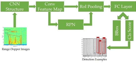
2.1. Faster R-CNN
2.2. Architecture
- we use the pretrained model to finetune the RPN module for region proposal task;
- we use those region proposals to train the Fast R-CNN, which is also pretrained by the same model for detection task;
- we fix the parameters in the convolutional layers and modulate the second RPN after initializing it by the above detection module, in which the sharing of convolutional computation is completed;
- we repeat step 3 but finetune the parameters, especially those belonging to the second Fast R-CNN.
2.3. Create a Convolution Neural Network
3. Detection Method Based on Faster R-CNN
4. Experiments and Results
4.1. Dataset
4.2. Specific Process
4.3. Comparison
4.3.1. R-CNN
4.3.2. Classification
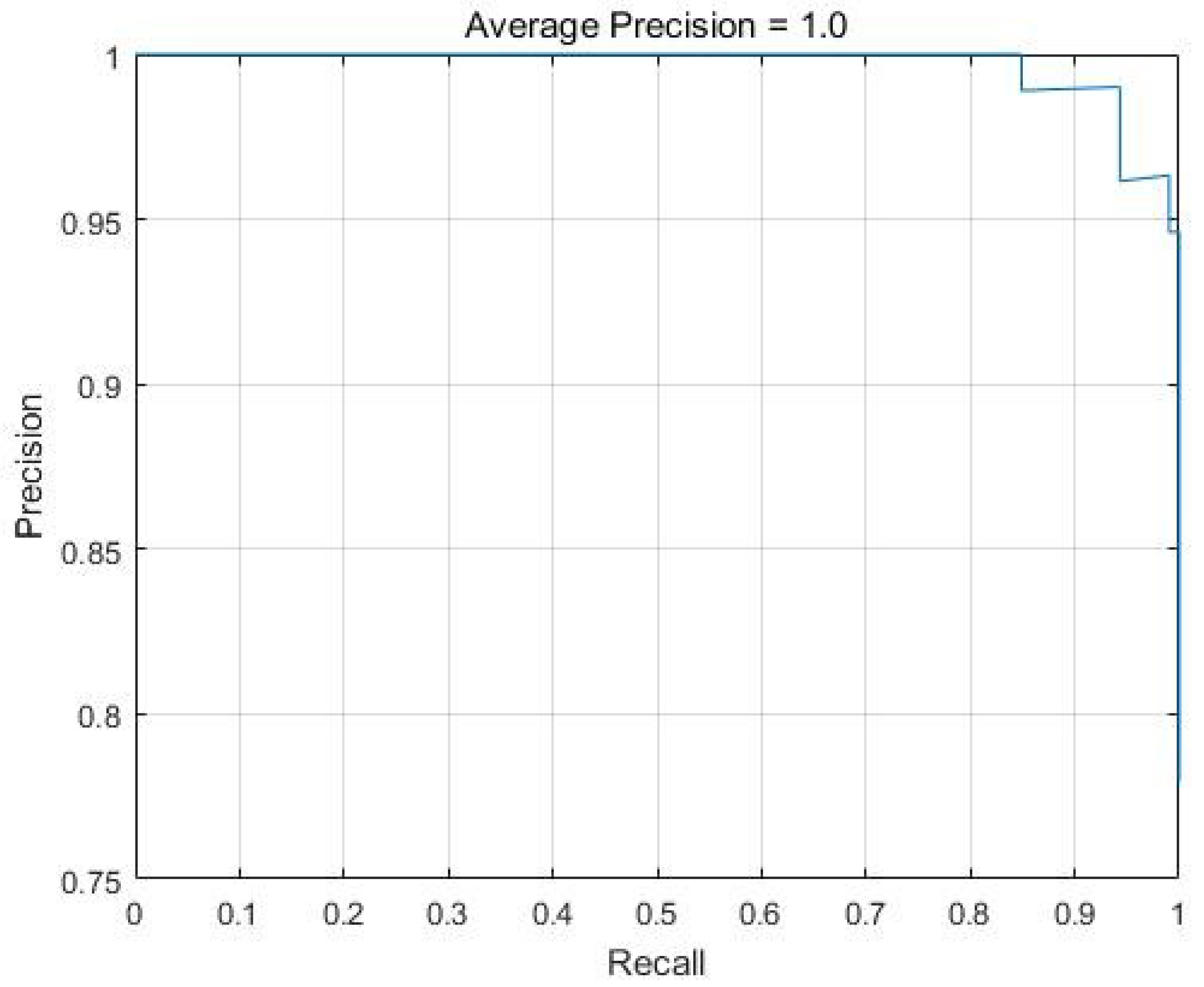
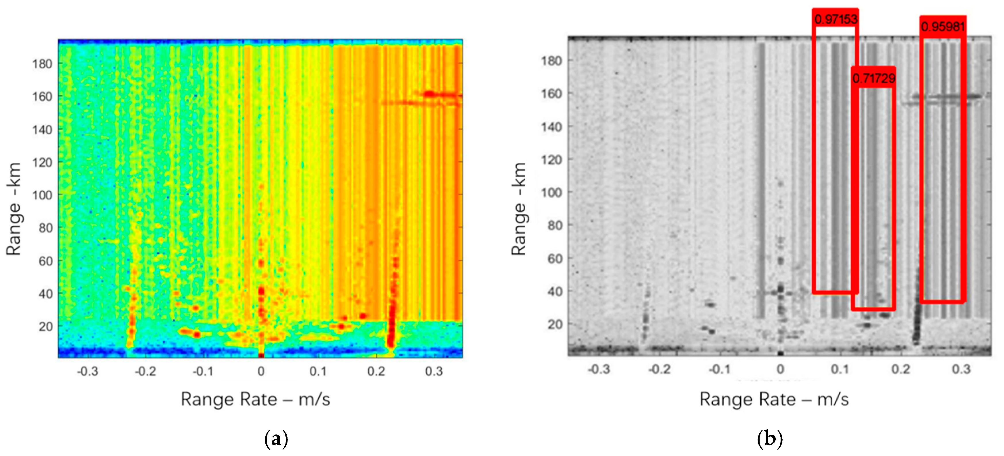
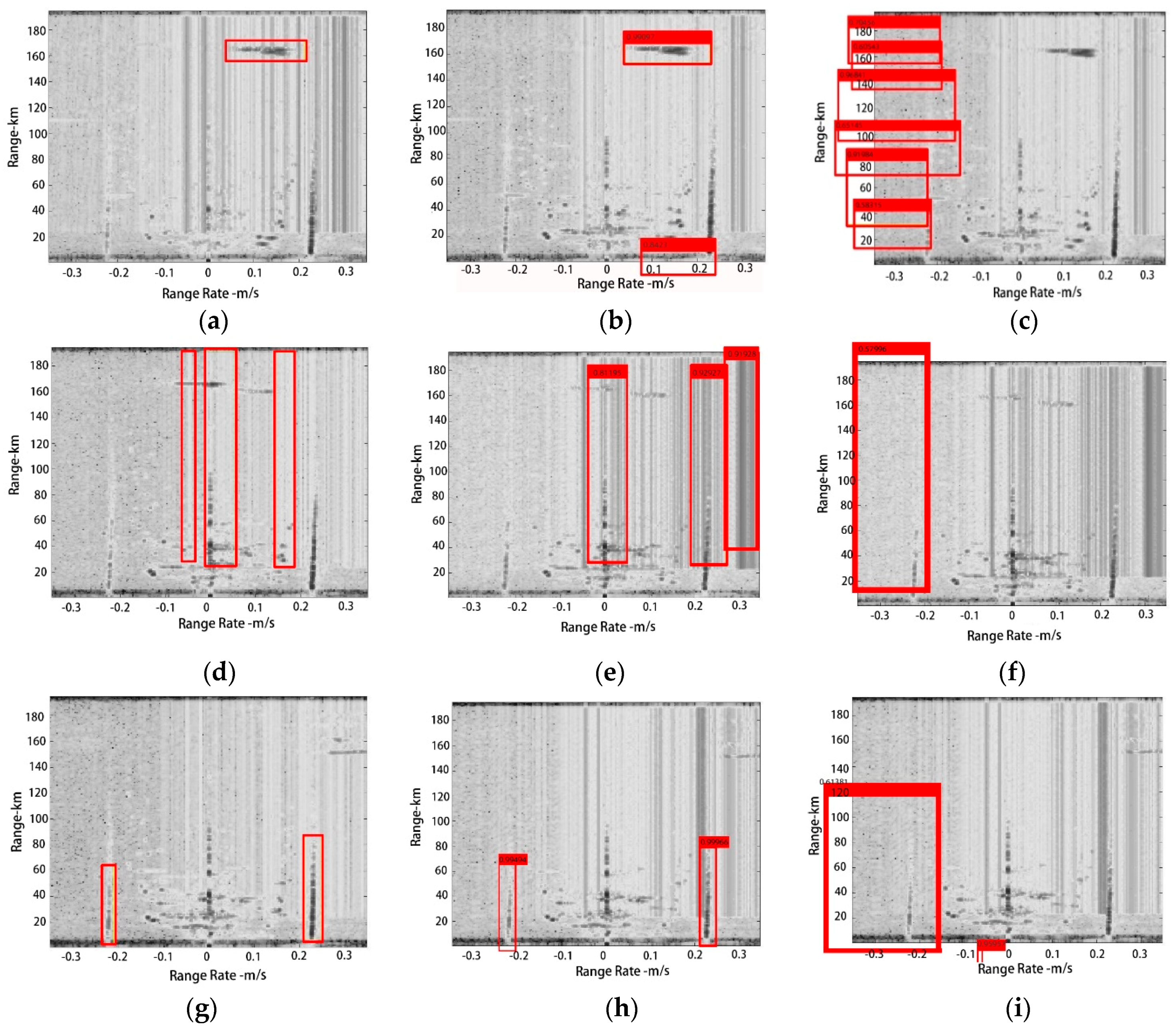
4.3.3. Detection
5. Discussion
6. Conclusions
Author Contributions
Funding
Acknowledgments
Conflicts of Interest
References
- Ponsford, A.M.; Wang, J. A review of high frequency surface wave radar for detection and tracking of ships. Turk. J. Electr. Eng. Comput. Sci. 2010, 18. [Google Scholar] [CrossRef]
- Zhang, L.; Li, M.; Niu, J.; Ji, Y. Ionospheric clutter extraction in HFSWR based on range-doppler spectral image processing. In Proceedings of the 2014 IEEE International Conference on Communication Problem-Solving, Beijing, China, 5–7 October 2014; pp. 615–618. [Google Scholar]
- Zhao, K.R.; Zhou, G.J.; Yu, C.J.; Quan, T.F. Target flying mode identification and altitude estimation in Bistatic T/R-R HFSWR. In Proceedings of the 17th International Conference on Information Fusion (FUSION), Salamanca, Spain, 7–10 July 2014; pp. 1–8. [Google Scholar]
- Yao, G.W.; Xie, J.H.; Ji, Z.Y.; Sun, M.L. The first-order ocean surface cross section for shipborne HFSWR with rotation motion. In Proceedings of the 2017 IEEE Radar Conference (RadarConf), Seattle, WA, USA, 8–12 May 2017; pp. 0447–0450. [Google Scholar]
- Li, R.; Hu, Z.; Hartnett, M. Short-Term forecasting of coastal surface currents using high frequency radar data and artificial neural networks. Remote Sens. 2018, 10, 850. [Google Scholar]
- Li, M.; Zhang, L.; Wu, X.B.; Yue, X.C.; Emery, W.J.; Yi, X.Z.; Liu, J.F.; Yang, G.B. Ocean surface current extraction scheme with high-frequency distributed hybrid sky-surface wave radar system. Trans. Geosci. Remote Sens. 2018, 56, 4678–4690. [Google Scholar] [CrossRef]
- Liu, Y.G.; Weisberg, R.H.; Merz, C.R. Assessment of CODAR and WERA HF radars in mapping currents on the West Florida Shelf. J. Atmos. Ocean. Technol. 2014, 31, 1363–1382. [Google Scholar] [CrossRef]
- Merz, C.R.; Liu, Y.G.; Gurgel, K.W.; Petersen, L.; Weisberg, R.H. Effect of radio frequency interference (RFI) noise energy on WERA performance using the “listen before talk” adaptive noise procedure. Coast. Ocean Obs. Syst. 2015, 229–247. [Google Scholar] [CrossRef]
- Zhao, C.; Xie, F.; Zhao, C.; He, C. Radio frequency interference mitigation for high-frequency surface wave radar. IEEE Geosci. Remote Sens. Lett. 2018, 15, 986–990. [Google Scholar] [CrossRef]
- Jangal, F.; Saillant, S.; Helier, M. Wavelet contribution to remote sensing of the sea and target detection for a high-frequency surface wave radar. IEEE Geosci. Remote Sens. Lett. 2008, 5, 552–556. [Google Scholar] [CrossRef]
- Chen, X.; Wu, X.; Liu, J.; Zhang, L. Interference detection method based on correspondence analysis for high frequency ground wave radar. Chin. J. Radio Sci. 2015, 30, 172–176. [Google Scholar]
- Jin, Z.L.; Pan, Q.; Liang, Y.; Cheng, Y.M.; Zhou, W.T. SVM-based land/sea clutter identification with multi-features. In Proceedings of the 31st Chinese Control Conference, Hefei, China, 25–27 July 2012; pp. 3903–3908. [Google Scholar]
- Li, Y.; Yang, Q.; Zhang, N. Ship detection with adaptive parameter based on detection background analysis. In Proceedings of the 2009 International Conference on Microwave Technology and Computational Electromagnetics (ICMTCE 2009), Beijing, China, 3–6 November 2009; pp. 486–489. [Google Scholar]
- Li, Y.; Zeng, W.J.; Zhang, N.; Tang, W.Y. Gabor feature based ionospheric clutter region extraction in Range-Doppler map. In Proceedings of the 2014 IEEE Antennas and Propagation Society International Symposium (APSURSI), Memphis, TN, USA, 6–11 July 2014; pp. 269–270. [Google Scholar]
- Li, Y.; He, M.K.; Zhang, N. An ionospheric clutter recognition method based on machine learning. In Proceedings of the 2017 IEEE International Symposium on Antennas and Propagation & USNC/UNSI National Radio Science Meeting, San Diego, CA, USA, 9–14 July 2017; pp. 1637–1638. [Google Scholar]
- Krizhevsky, A.; Sutskever, I.; Hinton, G.E. ImageNet classification with deep convolutional neural networks. Adv. Neural Inf. Process. Syst. 2012, 1, 1–9. [Google Scholar] [CrossRef]
- Zeiler, M.D.; Krishnan, D.; Taylor, G.W.; Fergus, R. Deconvolutional networks. In Proceedings of the 2010 IEEE Computer Society Conference on Computer Vision and Pattern Recognition, San Francisco, CA, USA, 13–18 June 2010; pp. 2528–2535. [Google Scholar]
- Karen, S.; Andrew, Z. Very deep convolutional networks for large-scale image recognition. arXiv, 2014; arXiv:1409.1556. [Google Scholar]
- Ren, S.Q.; He, K.M.; Girshick, R.; Sun, J. Faster R-CNN: Towards real-time object detection with region proposal networks. IEEE Trans. Pattern Anal. Mach. Int. 2017, 39, 1137–1149. [Google Scholar] [CrossRef] [PubMed]
- Zhang, Q.C.; Laurence, T.Y.; Chen, Z.K.; Li, P. A survey on deep learning for big data. Inf. Fusion 2018, 42, 146–157. [Google Scholar] [CrossRef]
- Liu, X.Y.; Wang, X.D. LS-decomposition for robust recovery of sensory big data. IEEE Trans. Big Data 2017. [Google Scholar] [CrossRef]
- Ji, Y.G.; Zhang, J.; Chu, X.L.; Sun, W.F.; Liu, A.J.; Niu, J.; Yu, C.J.; Li, M.; Wang, Y.M.; Zhang, L. A small array HFSWR system for ship surveillance. In Proceedings of the IET International Radar Conference 2015, Hangzhou, China, 14–16 October 2015; pp. 1–5. [Google Scholar]
- Girshick, R.; Donahue, J.; Darrell, T.; Malik, J. Rich feature hierarchies for accurate object detection and semantic segmentation. In Proceedings of the 2014 IEEE Conference on Computer Vision and Pattern Recognition, Columbus, OH, USA, 24–27 June 2014; pp. 580–587. [Google Scholar]


| Layer | Layer Name | Specific Operation |
|---|---|---|
| 1 | Image Input | 32 × 32 × 3 images with zerocenter normalization |
| 2 | Convolution | 32 × 3 × 3 convolutions with stride [1 1] and padding [1 1 1 1] |
| 3 | ReLu | ReLu |
| 4 | Convolution | 32 × 3 × 3 convolutions with stride [1 1] and padding [1 1 1 1] |
| 5 | ReLu | ReLu |
| 6 | Maxpooling | 3 × 3 max pooling with stride [2 2] and padding [0 0 0 0] |
| 7 | Fully Connected | 64 fully connected layers |
| 8 | ReLu | ReLu |
| 9 | Fully Connected | 2 fully connected layers |
| 10 | Softmax | Softmax |
| 11 | Classification Output | Crossentropyex |
| Layer | Layer Name | Specific Operation |
|---|---|---|
| 1 | Image Input | 32 × 32 × 3 images with zerocenter normalization |
| 2 | Convolution | 32 × 5 × 5 convolutions with stride [1 1] and padding [2 2 2 2] |
| 3 | ReLU | ReLU |
| 4 | Max Pooling | 3 × 3 max pooling with stride [2 2] and padding [0 0 0 0] |
| 5 | Convolution | 32 × 5 × 5 convolutions with stride [1 1] and padding [2 2 2 2] |
| 6 | ReLU | ReLU |
| 7 | Max Pooling | 3 × 3 max pooling with stride [2 2] and padding [0 0 0 0] |
| 8 | Convolution | 64 × 5 × 5 convolutions with stride [1 1] and padding [2 2 2 2] |
| 9 | ReLU | ReLU |
| 10 | Max Pooling | 3 × 3 max pooling with stride [2 2] and padding [0 0 0 0] |
| 11 | Fully Connected | 64 fully connected layers |
| 12 | ReLU | ReLU |
| 13 | Fully Connected | 10 fully connected layers |
| 14 | Softmax | Softmax |
| 15 | Classification Output | Crossentropyex |
| Feature Name. | Model | TP | TN | FP | FN | Precision | Recall | Accuracy |
|---|---|---|---|---|---|---|---|---|
| RFI | R-CNN | 102 | - | - | 22 | 1.0 | 0.8226 | 0.8226 |
| RFI | Faster R-CNN | 78 | - | - | 46 | 1.0 | 0.6290 | 0.6290 |
| seaClutter | R-CNN | 124 | - | - | - | 1.0 | 1.0 | 1.0 |
| seaClutter | Faster R-CNN | 124 | - | - | - | 1.0 | 1.0 | 1.0 |
| ioClutter | R-CNN | 122 | - | 2 | - | 0.9839 | 1.0 | 0.9839 |
| ioClutter | Faster R-CNN | 122 | - | 2 | - | 0.9839 | 1.0 | 0.9839 |
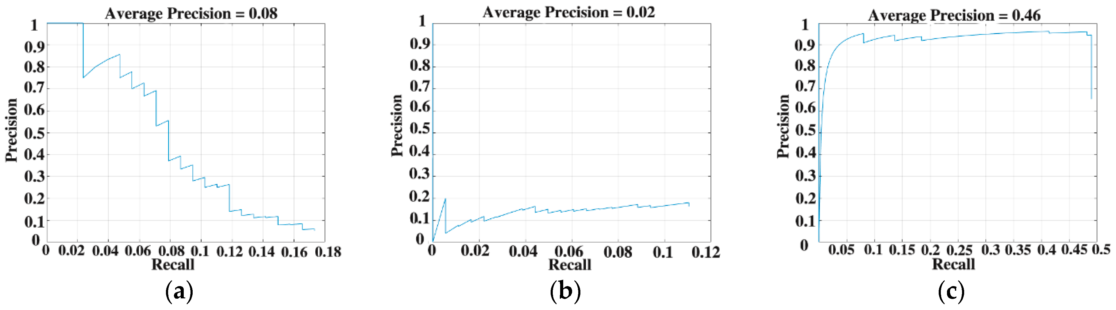
| Feature Name | Model | AP |
|---|---|---|
| RFI | R-CNN | 0 |
| RFI | Faster R-CNN | 0.0165 |
| ioClutter | R-CNN | 0 |
| ioClutter | Faster R-CNN | 0.0831 |
| seaClutter | R-CNN | 0 |
| seaClutter | Faster R-CNN | 0.4566 |
© 2018 by the authors. Licensee MDPI, Basel, Switzerland. This article is an open access article distributed under the terms and conditions of the Creative Commons Attribution (CC BY) license (http://creativecommons.org/licenses/by/4.0/).
Share and Cite
Zhang, L.; You, W.; Wu, Q.M.J.; Qi, S.; Ji, Y. Deep Learning-Based Automatic Clutter/Interference Detection for HFSWR. Remote Sens. 2018, 10, 1517. https://doi.org/10.3390/rs10101517
Zhang L, You W, Wu QMJ, Qi S, Ji Y. Deep Learning-Based Automatic Clutter/Interference Detection for HFSWR. Remote Sensing. 2018; 10(10):1517. https://doi.org/10.3390/rs10101517
Chicago/Turabian StyleZhang, Ling, Wei You, Q. M. Jonathan Wu, Shengbo Qi, and Yonggang Ji. 2018. "Deep Learning-Based Automatic Clutter/Interference Detection for HFSWR" Remote Sensing 10, no. 10: 1517. https://doi.org/10.3390/rs10101517
APA StyleZhang, L., You, W., Wu, Q. M. J., Qi, S., & Ji, Y. (2018). Deep Learning-Based Automatic Clutter/Interference Detection for HFSWR. Remote Sensing, 10(10), 1517. https://doi.org/10.3390/rs10101517