Performance and Requirements of GEO SAR Systems in the Presence of Radio Frequency Interferences

Abstract

Geosynchronous Synthetic Aperture Radar (GEO SAR) is a possible next generation SAR system, which has the excellent performance of less than one-day revisit and hundreds of kilometres coverage. However, Radio Frequency Interference (RFI) is a serious problem, because the specified primary allocation frequencies are shared by the increasing number of microwave devices. More seriously, as the high orbit of GEO SAR makes the system have a very large imaging swath, the RFI signals all over the illuminated continent will interfere and deteriorate the GEO SAR signal. Aimed at the RFI impact in GEO SAR case, this paper focuses on the performance evaluation and the system design requirement of GEO SAR in the presence of RFI impact. Under the RFI impact, Signal-to-Interference-plus-Noise Ratio (SINR) and the required power are theoretically deduced both for the ground RFI and the bistatic scattering RFI cases. Based on the theoretical analysis, performance evaluations of the GEO SAR design examples in the presence of RFI are conducted. The results show that higher RFI intensity and lower working frequency will make the GEO SAR have a higher power requirement for compensating the RFI impact. Moreover, specular RFI bistatic scattering will give rise to the extremely serious impact on GEO SAR, which needs incredible power requirements for compensations. At last, real RFI signal behaviours and statistical analyses based on the SMOS satellite, Beidou-2 navigation satellite and Sentinel-1 A data have been given in the appendix.

1. Introduction

L band, C band and X band spaceborne microwave systems play important roles in lots of remote sensing applications, such as the surface deformation measurements of landslides and earthquakes and vegetation mapping of forests. Nevertheless, the available microwave frequencies allocated for the spaceborne systems, called the active primary allocation frequencies, are given by the International Telecommunications Union’s (ITU’s) Earth Exploration-Satellite Service (EESS) [1]. Active primary allocations within the microwave frequency extension from L band to X band are provided in

Table 1. Active EESS primary allocations in L, C and X bands.

Band	Frequency Range (MHz)	Services in Band
L	1215–1300	Radio Navigation Satellite System (RNSS) and radiolocation
C	5250–5570	Aeronautical RNSS and radiolocation
X	9300–9900	Radiolocation and radio navigation

[1]. Beyond the primary allocation frequencies in different radio frequency bands, there are protected frequency bands or void frequency bands. Taking a classical protected frequency band in L band as an example, the frequency interval 1400–1427 MHz is protected, within which unwanted emissions of active service operations are forbidden and even the emissions from the nearby bands should be guaranteed to be lower than an expected value [2].

However, as more and more microwave devices are implemented, the primary allocation frequencies are becoming increasingly crowded. Different systems, which utilize the same or adjacent microwave frequency bands, will interfere with each other. Since only the active primary allocation frequencies can be used by the spaceborne microwave systems, the systems cannot avoid being impacted by the Radio Frequency Interference (RFI). Based on L band Aquarius scatterometers and the SMOS radiometer, strong RFI emissions, which might come from the terrestrial sources (e.g., military radars), have been detected [2,3,4]. Besides those detected by the radiometers, in 2016, Pascual et al. discussed the crosstalk RFI in the interferometric Global Navigation Satellite System Reflectometry (iGNSS-R), when the Delay-Doppler Map of the desired satellite is overlapped by other satellites [5]. Other detailed discussions about the classification of RFI sources, impacts analysis and mitigation methods in the global navigation satellite system (GNSS) system case were given in [6].

RFI is a common and serious problem in Synthetic Aperture Radar (SAR) as well. RFI decreases the SAR image quality by generating the noise-like artefacts, which is shown in Figure 1. RFI can also cause the saturation of the SAR echo and even produce spurious targets in the images [7]. Lots of RFI has been detected by SAR systems of different working bands. With respect to the L band SAR, the impact of RFI has been observed in ALOS-1 PALSAR data, which showed that RFI could not only cause haze-like image artefacts, linear pattern or blurs in the focused SAR image but reduce the capability of obtaining polarimetric signatures and the phase accuracies of SAR images [8]. Likewise, for C band systems, the RFI deriving from the Radio Local Area Networks (RLAN) could degrade the signals of the C band meteorological radars when the RFI power was comparable to that of the signal obtaining the nominal Signal-to-Noise Ratio (SNR) [9,10]. RFI signals could be observed affecting a few range lines in the C band Sentinel-1A SAR image [11]. Many low power RFI sources with the whole bandwidth and a few very high-power temporal RFIs are detected by Sentinel-1A SAR image as well [12]. Significantly, Radarsat-2 and Sentinel-1A have mutual interferences because they share the same working band and have the almost same equatorial crossing time and multiple repeat periods of each other. Although RFI signals in X band are not as obvious as those in C band, increased RFI mitigation capability is needed due to the wide designed bandwidth, as based on the analysis of the C- and X- band Windsat microwaves radiometer data [13,14]. Moreover, a small RFI modulated with a pulse wave has been observed in the X band TerraSAR-X system, which if notched out, will give rise to sidelobes in the SAR image [15]. Therefore, RFI is an important factor needed to be considered, including the future launched Geosynchronous orbit SAR (GEO SAR) system.

To improve the revisit and the coverage performance of the spaceborne SAR system, GEO SAR has been proposed [16]. Unlike a totally geostationary communication satellite, GEO SAR satellite runs in a geosynchronous orbit with non-zero inclination and eccentricity. Thus, a GEO SAR can obtain the relative movement with the targets on the ground, which ensures sufficient Doppler bandwidth after long time integration for realizing two-dimensional SAR imaging. It can achieve a revisit of the target region of one day and a wide beam footprint of more than hundreds of kilometres [17]. According to the inclination, the designed GEO SAR systems can be classified into the inclined orbit GEO SAR system (large inclination) and the quasi-geostationary system (small or zero inclination, small eccentricity but not zero) [18]. To satisfy the SNR requirement, inclined orbit GEO SAR system needs a higher power and a larger antenna size [19]. It achieves the designed azimuth resolution by a relative shorter integration time and it is sensitive to ionosphere and cluster disturbances [20,21,22,23,24,25,26,27,28]. In contrast, the geostationary system has lower requirements of the power and the antenna size [20]. Moreover, it has better revisit and observation performance for the target [29]. Nevertheless, it needs an integration time of hours. Thus, atmosphere distortion is a serious problem in this design [30]. GEO SAR has a longer integration time and a larger coverage compared with a Low Earth Orbit SAR (LEO SAR). Thus, it has an increased probability to be impacted by the RFI and the related impact will be more severe as well. Shown in Figure 2, the high orbit of GEO SAR gives rise to a large swath of about 400 km, while the swath of a LEO SAR is only around tens of kilometres in across track. Resultantly, more RFI signals will come into the beam of GEO SAR, compared with that in a LEO SAR case. Although the RFI impact depends on its time-frequency characteristics, such as the bandwidth and the transmitting duration, it is general noise-like, which can finally decrease the imaging quality of GEO SAR images by reducing the Signal-to-Interference-plus-Noise Ratio (SINR). Therefore, we need to consider and evaluate the RFI impact in the GEO SAR system design.

The paper is organized as follows. The RFI impact on the SINR and the required average transmitted power to compensate RFI impacts in the GEO SAR case are discussed in Section 2. In Section 3, focusing on the bistatic scattering RFI case, the RFI impact on SINR and the required transmitted powers in the specular scattering and non-specular scattering cases are studied. Moreover, under the assumption of the point-like target case, the Doppler filtering effect in the LEO SAR bistatic scattering RFI case is specially analysed. In Section 4, in the presence of the RFI, simulations are conducted to analyse the GEO SAR system design requirements in detail. Finally, Section 5 concludes this paper. In addition, some important real RFI measurement results in different frequencies are given in the Appendix.

2. Ground RFI Impacts on GEO SAR Signal

The ground RFI is the most common case which often derives from ground implemented radio electronic devices and ground-based radar systems. Thus, we analyse its impact on GEO SAR in this section. A sketch of a GEO SAR system in the presence of RFI is shown in Figure 3. The received RFI signal will raise the noise floor and degrade the Signal-to-Interference Ratio (SIR). Generally, the definition of the SIR is [32].

$$SIR=\frac{P_s}{P_{RFI}},$$

(1)

where $P_{RFI}$ is the power of the RFI and $P_s$ is the power of the received effective GEO SAR signal. Based on the radar equation [29], $P_s$ can be written as

$$P_s\left({\theta }_d,\psi \right)=\frac{P_a{A_t}^2{F}^2\left({\theta }_d,\psi \right)L_{loss}^2}{4\pi {\lambda }^2{R}^4}{\sigma }_0{\rho }_a{\rho }_g,$$

(2)

where $P_a$ is the average transmitted power of the GEO SAR signal, $A_t$ is its antenna aperture area, $F$ represents the gain, ${\theta }_d$ and $\psi$ represent the pointing direction of the antenna, $L_{loss}$ is the one-way total loss, ${\sigma }_0$ is the backscatter coefficient of the target, $\lambda$ is the wavelength, $R$ is the slant range and ${\rho }_a$ and ${\rho }_g$ are azimuth resolution and the ground range resolution, respectively.

Considering the thermal noise, we can define the SINR as

$$SINR=\frac{P_s}{P_{RFI}+P_{th}},$$

(3)

where $P_{th}$ is the power of the thermal noise, which can be written as [32]

$$P_{th}=k_B{T}_{th}{B}_g,$$

(4)

where $k_B=1.38\times {10}^{-23}J/K$ is the Boltzmann constant, $T_{th}$ is the thermal noise temperature and $B_g$ is the bandwidth of the GEO SAR system.

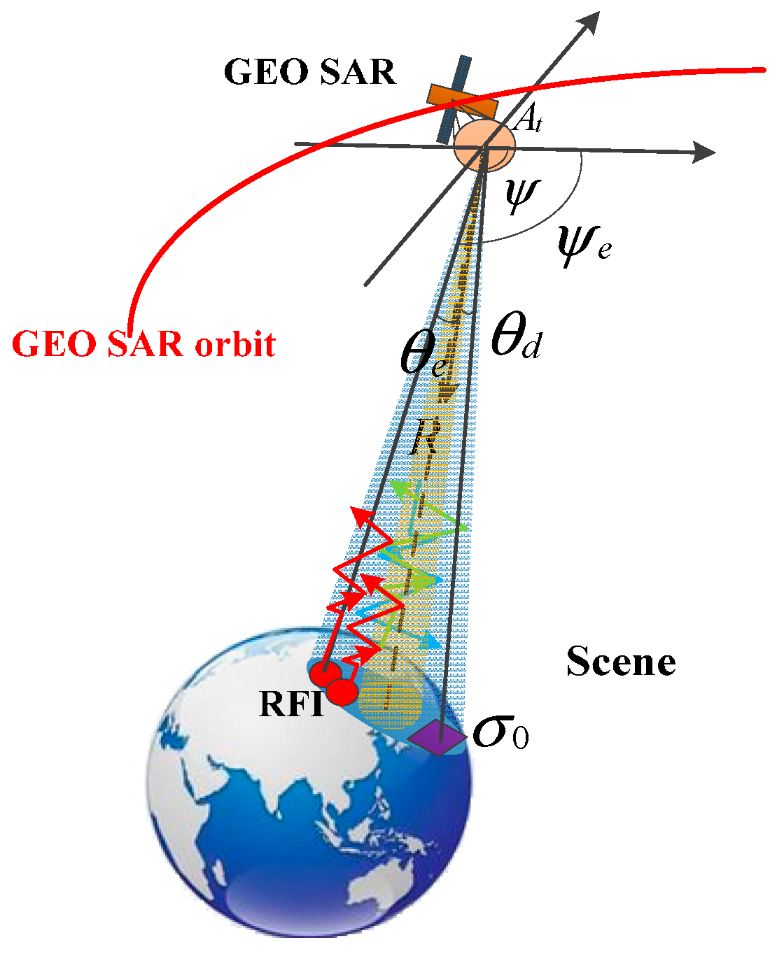
2.1. Point-Like RFI Source

If the ground RFIs are contributed by the point–like RFI sources (strong, localized and continuous emitting) [8,33], the powers of all the received point-source RFIs have to be summed together. Referring to Figure 3, the total power of RFI at the receiver of GEO SAR can be expressed as

$$P_{RFI}=\frac{A_t}{4\pi R^2}\cdot {\displaystyle \sum _{i=1}^N{P}_{e,i}{p}_{e,i}}F\left({\theta }_{e,i},{\psi }_{e,i}\right),$$

(5)

where $P_e$ is defined as the average Effective Isotropic Radiated Power (EIRP) of each single point-like RFI source, $p$ is the probability of each point-like RFI source, $i$ is the index, $N$ is the number of the point-like RFI sources, ${\theta }_e$ and ${\psi }_e$ indicates the position of each point-like RFI source. Because (5) relates to the antenna pattern, the position of the point-like RFI source will impact the power of $P_{RFI}$. A high-power point-like RFI source located far away from the centre of the beam of GEO SAR may have a smaller impact than a lower power point-like RFI source which is near the centre of the beam of GEO SAR.

2.2. Distributed RFI Source

Practically, many RFI sources on the ground are similar and independent distributed within a fixed area (e.g., personal electronic devices). Therefore, in this case, the emission of the RFI is noise-like, which is very similar to a black-body.

According to the basic theory of the black-body in microwave spectrum, under the assumption that the antenna receives the full EM field illuminated by the black-body, the antenna directivity within the solid angle is uniform and the bandwidth is small compared with the carrier frequency, we have [32]

$$P_{RFI}=k_B{B}_g{T}_{RFI},$$

(6)

where $T_{RFI}$ is the brightness temperature contributed by the distributed RFI sources. As the antenna area and the area of the beam foot-print are in the inverse proportion, $P_I$ will be independent on the antenna area. It only depends on the brightness temperature contributed by the RFI and the bandwidth of the receiver.

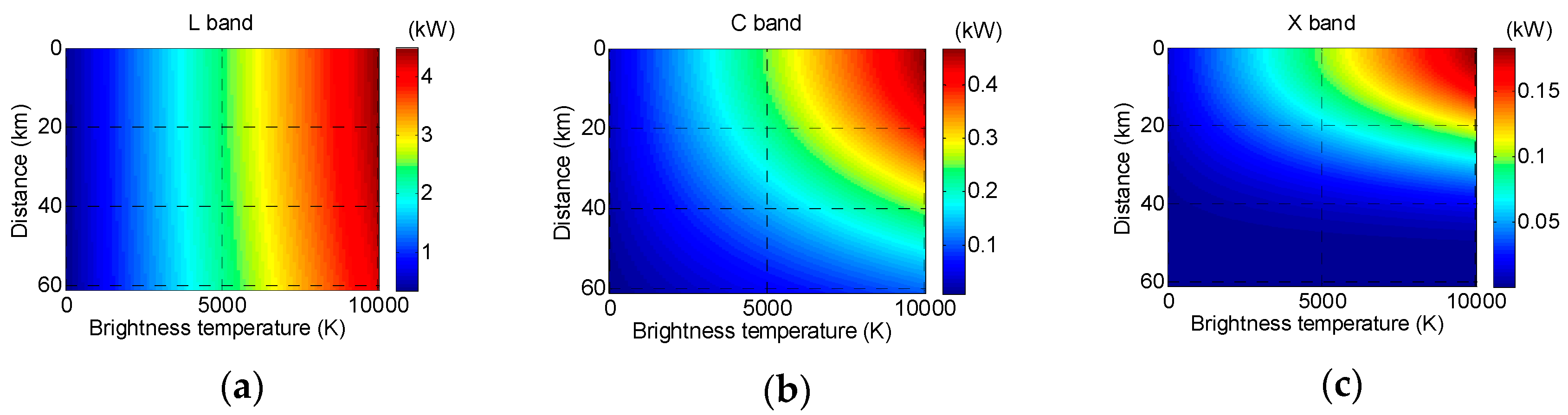
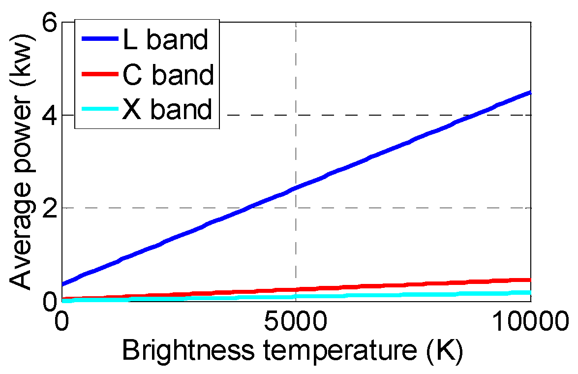
2.3. Average Transmitted Power Requirements in the Presence of RFI

RFI will degrade the SINR performance of a fixed GEO SAR system (e.g., specified average transmitted power, antenna size). To meet the requirements for achieving the good performances of remote sensing applications, we should determine the proper average transmitted power.

Considering the incoherent RFI and combining (2), the Noise-Equivalent Sigma Zero (NESZ) $NES{Z}_T$ can be expressed as

$$NES{Z}_T\left({\theta }_d,\psi \right)=\frac{4\pi R^4{\lambda }^2{k}_B\left(T_{RFI}+T_{th}\right)}{P_a{A_t}^2{F}^2\left({\theta }_d,\psi \right)L_{loss}^2{T}_a{\rho }_a{\rho }_g},$$

(7)

where, especially, in the multi point-like RFI source case,

$$T_{RFI}=\frac{h_I{A}_t}{4\pi k_B{R}^2},$$

(8)

is the RFI equivalent brightness temperature, $h_I={\displaystyle \sum _{i=1}^N\frac{P_{e,i}{p}_{e,i}F\left({\theta }_{e,i},{\psi }_{e,i}\right)}{B_{I,i}}}$ is the power spectrum density, $B_I$ is the bandwidth of the point-like RFI source and $T_a$ is the integration time of GEO SAR. In the distributed RFI source case, $T_{RFI}$ is the brightness temperature caused by the noise-like RFI.

Based on (7), in both the point-like RFI source case and the distributed RFI source case, the SINR will have the following relationship in dB

$$SINR={\sigma }_0-NES{Z}_T,$$

(9)

According to (9), with respect to the fixed target (specified ${\sigma }_0$), to satisfy the SINR requirement for SAR applications with a good performance (e.g., to keep the SINR above 10 dB in SAR interferometry applications for making the coherence of the interferogram above 0.9 [34]), we should design the average transmitted power of the GEO SAR system as

$$P_{ar}=\frac{4\pi {\lambda }^2{R}^4{k}_B(T_{RFI}+T_{th})SIN{R}_r}{{A_t}^2{L}_{loss}^2{T}_a{\rho }_a{\rho }_g{\sigma }_0},$$

(10)

where $P_{ar}$ is the required average transmitted power of GEO SAR and $SIN{R}_r$ is the required SINR.

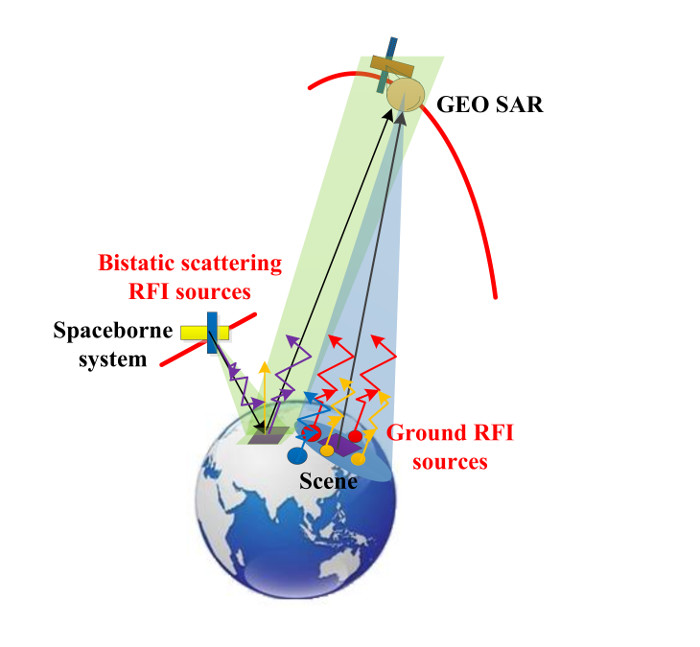
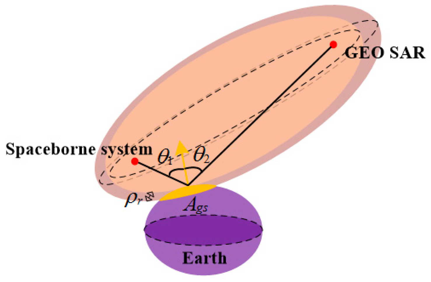
3. Bistatic Scattering RFI Impact on GEO SAR

3.1. Impact of Bistatic Scattering RFI on GEO SAR

Besides the RFI impacts coming from the ground RFI directly, some other received RFI signals may derive from the signals emitted from spaceborne radio systems (e.g., LEO SAR and GNSS satellite system) with the same or adjacent radio frequencies and bistatic scattering from the ground [6,35,36,37]. The sketch of the impact of the bistatic scattering RFI case on GEO SAR is shown in Figure 4. $P_{ia}$ is the average transmitted power of the spaceborne radio system (RFI source), $O$ represents the position of the target, $L$ is the position of the spaceborne system, $R_s$ is the slant range of the spaceborne systems, ${\widehat{R}}_s$ is the unit vector from $O$ to $L$, $S$ is the position of GEO SAR, $R$ is the range of the GEO SAR, $\widehat{R}$ is the unit vector from $O$ to $S$, ${\theta }_1$ is the incidence angle of the spaceborne system and ${\theta }_2$ is the corresponding RFI bistatic scattering angle to GEO SAR, $\widehat{z}$ is the normal unit vector of the scene, $\widehat{x}$ is the unit vector of the projection of ${\widehat{R}}_s$ on the scene plane, $\widehat{y}$ is determined by the cross product of orthonormal basis $\widehat{z}$ and $\widehat{x}$, ${\psi }_s$ is the out-of-plane angle of the bistatic scattering direction, $\beta$ is the bistatic angle which relates to ${\theta }_1$, ${\theta }_2$ and ${\psi }_s$, ${\sigma }_B^0$ is the bistatic scattering coefficient, ${\theta }_{RFI}$ is the beam width of the spaceborne system, ${\theta }_{GEO}$ is the beam width of the GEO SAR.

3.1.1. Non-Specular Bistatic Scattering Case

Generally, if the bistatic scattering signal does not form a specified angle to produce the specular scattering case, non-specular scattering occurs (out-of-plane case (${\theta }_1={\theta }_2,{\psi }_s\ne 0$) and in-plane case (${\theta }_1\ne {\theta }_2,{\psi }_s=0$)). For the out-of-plane case, ${\sigma }_B^0$ turns minimum when ${\psi }_s$ approaches 90° and ${\sigma }_B^0$ is almost same with that in the in-plane case when ${\psi }_s$ is near 0° or 180° [38]. Thus, if we consider the in-plane case for the worst condition, based on the constant-$\gamma$ bistatic-scatter-region model [38], in-plane land clutter bistatic scattering coefficient can be approximately expressed as

$${\sigma }_B^0=\gamma {\left(\sin {\theta }_1\sin {\theta }_2\right)}^{\raisebox{1ex}{$1$}\!\left/ \!\raisebox{-1ex}{$2$}\right.},$$

(11)

where $\gamma$ is the normalized reflectivity parameter, which can be estimated by

$$\gamma =\frac{{\sigma }_M^0}{\sin {\theta }_1}$$

(12)

where ${\sigma }_M^0$ is the monostatic scattering coefficient.

Regardless of the large-bistatic-angle case (e.g., forward-scatter region), we simply focus on the bistatic scattering case with the relative small bistatic angle for the above analysis. Such as for ALOS-2 PALSAR, the bistatic angle formed by the LEO SAR and the GEO SAR is general less than 30° when the LEO SAR signal is received by the GEO SAR within its antenna mainlobe. For the LEO SAR signal received outside the GEO SAR antenna mainlobe, as there will be a large attenuation for the RFI signal, we ignore the large-bistatic-angle case. Moreover, although the GNSS system and the GEO SAR can generate the bistatic system with large bistatic angle, because ${\sigma }_B^0$ is generally smaller than ${\sigma }_M^0$ [38], a small bistatic angle assumption is better for analysing the worst cases.

In the non-specular case, the received RFI signal is weak as the gain in the scattering direction of the GEO SAR is low.

3.1.2. Specular Bistatic Scattering Case

At times, if ${\theta }_1={\theta }_2$ and ${\psi }_s=0$, a specular reflection happens. In this case, the power of the RFI will concentrate in the scattering direction of GEO SAR and the received RFI signal from the spaceborne system is very strong. In the specular scattering case, like a mirror reflection [32,39], ${\sigma }_B^0$ can be expressed as

$${\sigma }_B^0=\frac{4\pi A_{gs}}{{\lambda }^2},$$

(13)

where $A_{gs}$ is the specular scattering area on the ground. Here and in the following part, we also use $\lambda$ as the wavelength of the spaceborne radio system for simplicity. As the targets within the same range resolution cannot be distinguished by the range delay difference, ideally, the maximum area of $A_{gs}$ can be approximately determined within the range resolution bin ${\rho }_r$ by the cross-section area between the ellipsoid formed by GEO SAR and the spaceborne system and the Earth ellipsoid, which has been shown in Figure 5.

Based on the above analysis, the considerably different behaviour of the two cases derives from the different bistatic scattering coefficients which are shown in (11) and (13). In the specular scattering case, the bistatic scattering coefficient is large, while it will be very small in the non-specular scattering case.

3.1.3. SINR and Required Power Analysis

In the bistatic scattering RFI case, the total brightness temperature $T_{RFI\_sa}$ can be shown as

$$T_{RFI\_sa}=\frac{1}{k_B}{\displaystyle \sum _{k=1}^{N_b}\frac{\frac{1}{T_o}{\displaystyle \underset{T_w}{\int }\left(\frac{P_{ia,k}}{{\left({\theta }_{RFI}{R}_s(t)\right)}^2}{\sigma }_{B,k}^0\left(t\right)A_s\frac{A_t}{4\pi R{(t)}^2}\right)p_{b,k}{L}_{lossb,k}F\left({\theta }_{di,k},{\psi }_{i,k},t\right)dt}}{B_{I,k}}},$$

(14)

where $P_{ia,k}$ is the average transmitted power of the kth spaceborne system, $A_s$ is the coverage area of the spaceborne system, $p_{b,k}$ is the corresponding illuminating probability for the bistatic scattering case, $T_o$ is the time period of one orbit for the spaceborne system, $T_w$ is the operation time of the spaceborne system per orbit, $L_{lossb}^{}$ is the transmitting loss of the RFI signal, $t$ is the slow time, $k$ is the index and $N_b$ is the number of the spaceborne systems. The integration in (14) refers to the variation of the bistatic scattering coefficient and the gain of GEO SAR towards the spaceborne system within the integration time of GEO SAR.

$A_s$ changes in different cases, when ${\theta }_{RFI}>{\theta }_{GEO}$ (e.g., GNSS system) or ${\theta }_{RFI}<{\theta }_{GEO}$(e.g., LEO SAR system), which can be shown as

$$A_s=\{\begin{array}{c}{\left({\theta }_{GEO}R\right)}^2,{\theta }_{RFI}>{\theta }_{GEO}\\ {\left({\theta }_{RFI}{R}_s\right)}^2,{\theta }_{RFI}<{\theta }_{GEO}\end{array}.$$

(15)

Based on (6) and (14), the SINR in the bistatic scattering RFI case can be written as

$$SINR\left({\theta }_d,\psi \right)=\frac{4\pi {\lambda }^2{R}^4{k}_B\left(T_{th}+T_{RFI\_sa}\right)}{P_a{A_t}^2{F}^2\left({\theta }_d,\psi \right)L_{loss}^2{T}_a{\rho }_a{\rho }_g{\sigma }_0}.$$

(16)

Likewise, being the same with (10), we can use (16) to obtain the average transmitted power requirement of GEO SAR $P_{ar}$ for meeting the required SINR in the presence of the spaceborne system RFI.

3.2. Doppler Filtering

Specially, if our interesting target is point-like and isolated, the received pulses will have deterministic phases. In this case, Doppler filtering on RFI signal will have a good performance to weaken the RFI impact. Figure 6a shows the geometry difference between GEO SAR and LEO SAR. $v_s$ and $v_g$ are the velocity vectors of the LEO SAR system and the GEO SAR system, respectively. Vectors $R_s$ and $R$ represent the incidence direction (line of sight (LOS)) and the bistatic scattering direction, respectively. $\vartheta$ is the LOS angle between $v_s$ and $R_s$. GEO SAR has a larger beam footprint (e.g., typically 400 km) than that of LEO SAR (e.g., typically 10 km in along-track). Moreover, the velocity of GEO SAR is small compared with that of a LEO SAR. Resultantly, the Doppler rate of GEO SAR is very small compared with that of a LEO SAR. To achieve the same azimuth resolution, the Doppler bandwidth of GEO SAR is much smaller (only dozens of Hz at most) than the Doppler bandwidth of a LEO SAR (hundreds to thousands Hz), which is shown in Figure 6b. Moreover, as the pulse repetition frequency (PRF) of GEO SAR is still smaller than the Doppler bandwidth of a LEO SAR, the Doppler frequency of a LEO SAR will be aliased. When doing the Doppler filtering in the imaging processing, a GEO system achieves the azimuth focusing by exploiting the small Doppler bandwidth. Therefore, the components of the LEO SAR RFI Doppler spectrum out of the Doppler bandwidth of GEO SAR could be filtered, as shown as the yellow regions in Figure 6b. It should be noticed that the aliased Doppler frequencies of the LEO SAR within the GEO SAR Doppler bandwidth cannot be filtered out.

As the integration time of GEO SAR (hundreds of second or even hours) is far longer than that in a LEO SAR (typically 1 s), if we assume the LEO SAR observes the target within the integration time of the GEO SAR in a worst case (like a staring mode), the LEO SAR signal can be simplified as weighted by the envelope of GEO SAR. Moreover, the worst geometry relationship between the GEO SAR and LEO SAR is assumed as well, which makes the RFI signal of LEO SAR be weighted by the GEO SAR antenna pattern. Under the assumption, the received RFI signal from the LEO SAR is expressed as

$$\begin{array}{cc}\hfill s_l\left(t\right)& =A\sin {\mathrm{c}}^2\left(\frac{v_g{L}_g}{\lambda R_0}t\right)\exp \left(j\frac{4\pi R_s\left(t\right)}{\lambda }\right)\hfill \\ \hfill & =A\sin {\mathrm{c}}^2\left(\frac{v_g{L}_g}{\lambda R_0}t\right)\exp \left[j\pi \left(\frac{4R_{0,l}}{\lambda }+f_{dc,l}t+f_{dr,l}{t}^2+\cdots \right)\right],\hfill \end{array}$$

(17)

where $A$ (relates to SINR) is the amplitude of the RFI, $L_g$ is the antenna size of GEO SAR, $v_g$ is the velocity of GEO SAR, $R_{0,l}$ is the shortest slant range of $R_s$, $f_{dr,l}$ is the Doppler rate of the LEO SAR, $f_{dc,l}^{}$ is the Doppler centroid frequency of the LEO SAR. Sinc function represents the envelope of the GEO SAR signal.

The received GEO SAR signal is

$$\begin{array}{cc}\hfill s_l\left(t\right)& =\sin {\mathrm{c}}^4\left(\frac{v_g{L}_g}{\lambda R_0}t\right)\exp \left(j\frac{4\pi R\left(t\right)}{\lambda }\right)\hfill \\ \hfill & =\sin {\mathrm{c}}^4\left(\frac{v_g{L}_g}{\lambda R_0}t\right)\exp \left[j\pi \left(\frac{4R_0}{\lambda }+f_{dc,g}t+f_{dr,g}{t}^2+\cdots \right)\right],\hfill \end{array}$$

(18)

where $R_0$ is the shortest slant range of GEO SAR, $f_{dr,g}$ is the Doppler rate of the GEO SAR, $f_{dc,g}$ is the Doppler centroid frequency of the GEO SAR.

The energy of the LEO SAR RFI signal $E$ after Doppler filtering is

$$E=A^2{{\displaystyle \underset{-\frac{T_a}{2}}{\overset{\frac{T_a}{2}}{\int }}\left|{\displaystyle \underset{-\frac{T_a}{2}}{\overset{\frac{T_a}{2}}{\int }}{\sin \mathrm{c}}^2\left(\frac{v_g{L}_g}{\lambda R_0}u\right)\exp \left[j\pi \left(\frac{4}{\lambda }{R}_{0,l}+f_{dc,l}u+f_{dr,l}{u}^2\right)\right]\cdot rect\left(\frac{t-u}{T_a}\right)\exp \left[-j\pi f_{dr,g}{\left(t-u\right)}^2\right]du}\right|}}^{2}dt.$$

(19)

Expanding the exponent terms and combining them, ignoring the impact of the antenna pattern for simplicity, we have

$$E\approx \frac{A^2}{\left|f_{dr,l}-f_{dr,g}\right|}{{\displaystyle \underset{-\frac{T_a}{2}}{\overset{\frac{T_a}{2}}{\int }}\left|\exp \left[j\frac{\pi }{\left(f_{dr,l}-f_{dr,g}\right)}{\left(\frac{f_{dc,l}-f_{dc,g}}{2}+f_{dr,g}t\right)}^2\right]\right|}}^{2}dt\approx \frac{A^2{T}_a}{\left|f_{dr,l}-f_{dr,g}\right|}.$$

(20)

In the meantime, the energy of the effective GEO SAR signal $E_m$ after Doppler filtering is expressed as

$$E_m={{\displaystyle \underset{\frac{-1}{f_{dc,g}{T}_a}}{\overset{\frac{1}{f_{dc,g}{T}_a}}{\int }}\left|{\displaystyle \underset{-\frac{T_a}{2}}{\overset{\frac{T_a}{2}}{\int }}{\sin \mathrm{c}}^4\left(\frac{v_g{L}_g}{\lambda R_0}u\right)\exp \left[j\pi \left(\frac{4}{\lambda }{R}_0+f_{dc,g}u+f_{dr,g}{u}^2\right)\right]\cdot rect\left(\frac{t-u}{T_a}\right)\exp \left[-j\pi f_{dr,g}{\left(t-u\right)}^2\right]du}\right|}}^{2}dt.$$

(21)

Simplifying the equation, we have

$$E_m\approx \frac{0.9T_a}{\left|f_{dr,g}\right|}.$$

(22)

The ratio between the energy of the GEO SAR signal and the energy of the RFI after Doppler filtering is shown as

$$\Re =\frac{E_m}{E}\approx \frac{0.9}{A^2}\frac{\left|f_{dr,l}-f_{dr,g}\right|}{\left|f_{dr,g}\right|}\cdot \frac{PR{F}_g}{f_{dr,l}{T}_a},$$

(23)

where $PR{F}_g$ is the pulse repetition frequency of GEO SAR. If GEO SAR uses a small PRF, the Doppler spectrum of the RFI will be aliased, leading to a small value of $\Re$, that, in turn results in a small SINR. The difference of the Doppler rates of GEO SAR and LEO SAR is the parameter to describe the attenuation of LEO SAR RFI signal after Doppler filtering. A higher difference between the Doppler rates of GEO SAR and LEO SAR will be helpful to raise $\Re$. A higher $\Re$ indicates a better imaging performance of GEO SAR in the presence of LEO SAR RFI.

In the case of the distributed target, the LEO SAR illuminates it with a PRF that causes the backscattered returns to be independent, white. The LEO-GEO bistatic scattering will then be nearly white and performance of the Doppler filtering will lose.

4. Performance Evaluation and Discussion: Example of GEO SAR Design

In this section, we evaluate the performance of GEO SAR in the presence of RFI by using System Tool Kit (STK) software to generate the GEO SAR orbit, LEO SAR orbits and the GNSS orbits for the simulation. The High-Precision Orbit Propagator (HPOP) in STK is adopted to obtain more accurate orbit simulation. The input parameters of our inclined orbit GEO SAR system are given in

Table 2. Classical parameters of the inclined orbit GEO SAR system.

Parameter	Value	Parameter	Value
Carrier central frequency (GHz)	1.25/5.4/9.6	Inclination (°)	10–60
Look angle (°)	2–7	Argument of perigee (°)	270
Eccentricity	0.07	Antenna area (m2)	531
Duty cycle (%)	15	Incidence angle (°)	10–60
Bandwidth (MHz)	18	Integration time (s)	30–250
Polarization	HH	Equivalent thermal noise (K)	879

[19,21]. We consider the classical “Figure 8” inclined GEO SAR orbit with the small eccentricity and the large inclination. The designed GEO SAR system can work in three frequency bands (L, C and X). The large antenna size is utilized to obtain the higher gain of the GEO SAR signal.

The performance of a GEO SAR defined in Table 2, is shown in

Table 3. Performance of GEO SAR system.

Parameter	Value	Parameter	Value
Number of beams	1 (L band) 16 (C band) 64 (X band)	SINR (dB)	10
Resolution (m)	<20 × <20 (Single look)	Coverage (km)	400 × 400

. We assume that both the antenna size and the swath are kept constant with different frequencies (from L band to X band), by using scan SAR mode. From Table 2, when the working frequency of GEO SAR increases from the L band to X band, the number of beams will accordingly change from 1 to 64 to keep the coverage requirement. We design the basic SINR requirement as 10 dB to make the system reach the imaging requirement for interferometric applications. Proper signal bandwidth and integration times make the GEO SAR system have range and azimuth resolutions better than 20m.

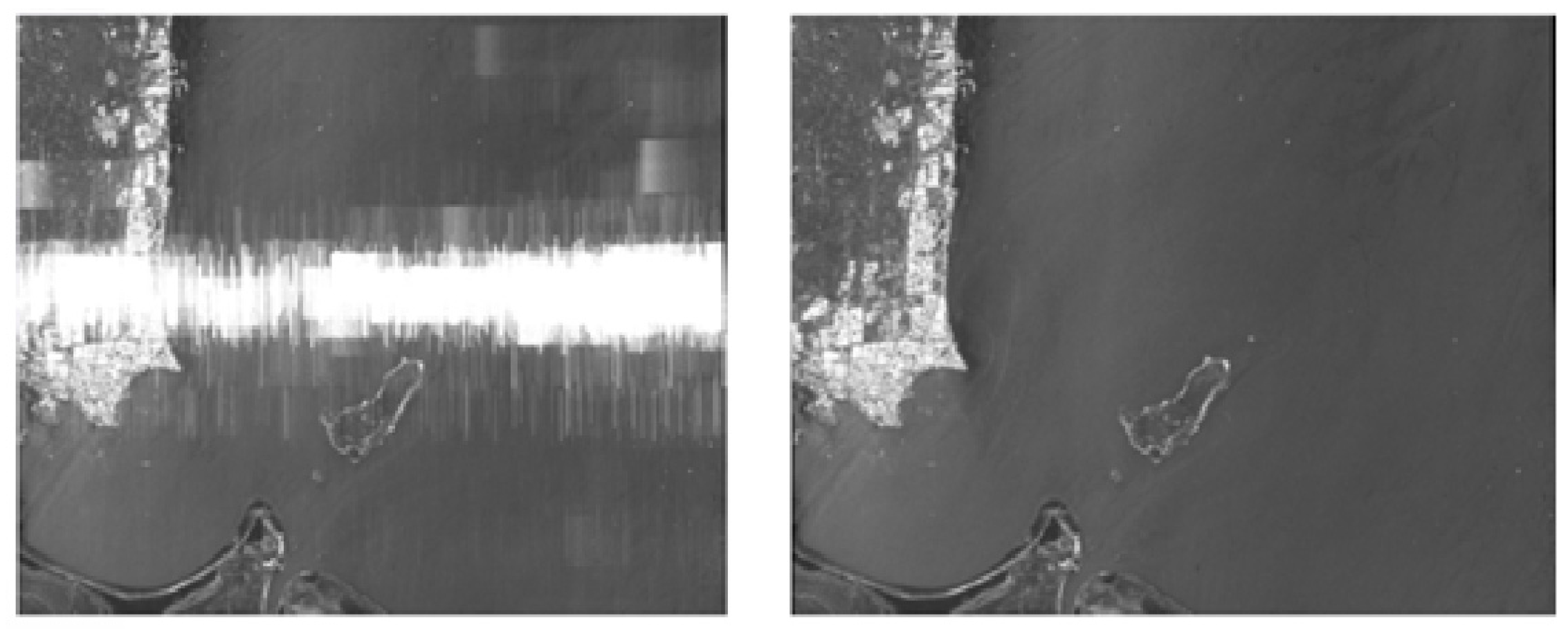
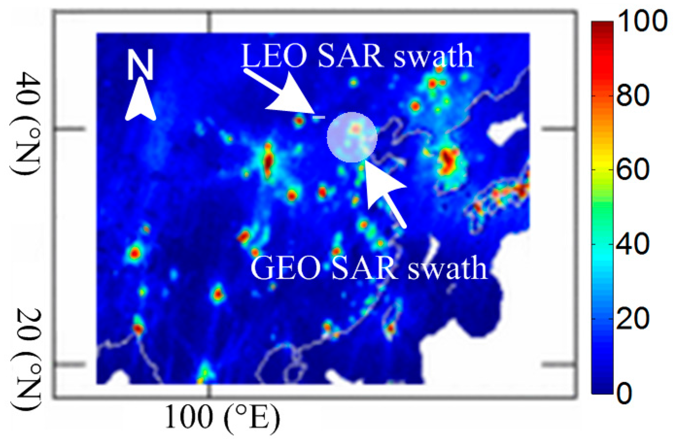
4.1. Impact of Ground RFI

In the simulation of the ground RFI case, the location of the beam centre of the GEO SAR is set in Beijing (40°N, 116°E), when the GEO SAR is at the orbit position of 162° true anomaly with a 2.6° look angle. Moreover, we assume the one-way signal loss of GEO SAR is 3 dB. According to the analysis of the real RFI data obtained by the spaceborne systems in the appendix, as the RFI brightness temperature is general thousands of Kelvin, the scope of the RFI brightness temperature in the analysis is from 0 to 10,000 K.

According to the SINR requirement in Table 3, the average transmitted power requirement of the GEO SAR system with the variation of RFI intensity and the distance from the position of the point-like RFI source to the beam centre of GEO SAR is shown in Figure 7. The average transmitted power requirements in all three working frequencies will increase with the increasing of the brightness temperature. In the meantime, the average transmitted power requirements are also very sensitive to the relative distance between the beam centre of GEO SAR and the position of the point-like RFI. When the distance increases, the average transmitted power requirement will decrease, because the power of the RFI after weighting by the antenna pattern of GEO SAR becomes small. Taking the L band system and the brightness temperature of 5000 K as an example, when the distance changes from 0 to 60 km, the average transmitted power requirements varies from more than 2.4 kW to less than 2.3 kW. At last, because of the shorter wavelength, the smaller beam width and the higher backscatter coefficient, comparing the three sub-figures in Figure 7, a higher frequency is helpful to reduce the required average transmitted power. Under the case of a 5000 K brightness temperature RFI and locating at 60 km away from the centre of the GEO SAR beam, the average transmitted power requirement changes from about 2.3 kW to only 0.2 W from L band to X band. Thus, an L band GEO SAR system needs a higher transmit power to compensate the RFI impact.

Likewise, shown in Figure 8, in the case of distributed RFI, the average transmitted power requirement will increase when the RFI brightness temperature turns higher. In the meantime, similarly, the GEO SAR system with a higher working frequency also has a much lower average transmitted power requirement in the distributed RFI case, which suggests the system will be easier to be implemented. Nevertheless, as the interference is uniform, the impact does not depend on the positions of the RFI and the beam centre of GEO SAR.

4.2. Impact of Bistatic Scattering RFI

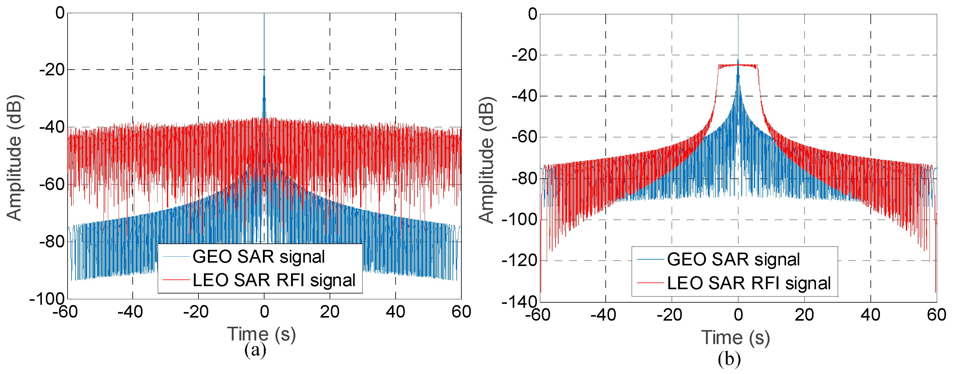
4.2.1. LEO SAR Bistatic Scattering RFI Case Analysis

In this part, we analyse the bistatic scattering RFI impacts of LEO SAR on GEO SAR. In

Table 4. Utilized system parameters of the main LEO SAR (L, C and X bands) in the simulation.

Frequency	L Band			C Band			X Band
SAR	ALOS-2	Tandem-L	SAOCOM-1A/B	Sentinel-1A/B	Radarsat-2	RCM	TanDEM-X/PAZ	COSMO-SkyMed	SAR-Lupe	KOMPSAT-5
Peak power (W)	5100	3622	3100	4368	2280	1600	2260	7600	250 (total)	1700
Duty cycle of power (%)	8	4	5	12	12	13.75	18	11		35
Orbit period (min)	98.5	99.7	97.2	98.5	100.7	96.4	95.0	20% (max)	20% (assumed)	95.8
Working time per orbit (min)	49	30	5–20	25, 74 (wave mode)	28	15	3			2
Satellite number	1	2	2	2	1	3	3	4	5	1
Average transmitted power (W)	203	44	32	394	76	34	13	167	50	13
Bandwidth (MHz)	42 (middle)	84	50	100	100	100	150/300	400	300 (assumed)	120

[40,41,42,43,44,45], the utilized system parameters of the main L band, C band and X band LEO SAR systems in the simulation are given, including most important parameters about the power and the orbit. It can be noted that the number of the LEO SAR systems is large, because some of the systems are formed by not only a single satellite but many satellites as a constellation.

The orbits of the ALOS-2 PALSAR, Sentinel-1 A and TerraSAR-X have been used as the examples of L-, C- and X band LEO SAR systems to calculate the occurrence probabilities of non-specular scattering case, specular scattering case and mainlobe to mainlobe specular scattering case by STK software. The analysis result of the occurrence probabilities is provided in

Table 5. Occurrence probability of the LEO SAR bistatic scattering RFI and the average transmitted power requirement in GEO SAR (HH polarization, Shrub scene, in the specular scattering case: ${\theta }_1={\theta }_2={30}^{\circ }$, in the non-specular case: ${\theta }_1={30}^{\circ },{\theta }_2={45}^{\circ }$).

Parameters			L	C	X
Occurrence probability (%)	Non-specular scattering		44.8	38.1	39.0
	Specular scattering		5.0 × 10−2	1.5 × 10−2	2.0 × 10−3
	Mainlobe to mainlobe specular scattering		0	0	0
σ0 (dB)			−14.8	−9.7	−7.6
Required average transmitted power (kW)	Non-specular scattering	0	0.7	6.0 × 10−2	2.0 × 10−2
		5000 km	0.7	5.2 × 10−2	1.8 × 10−2
	Specular scattering	0	1.1 × 109	3.2 × 107	4.7 × 105
		5000 km	2.4 × 104	7.8	3.7 × 10−2
	Mainlobe to mainlobe specular scattering		-	-	-

. The occurrence probabilities are obtained based on the orbit simulation of the GEO SAR and the LEO SAR with different periods, which are the repeat orbit cycles of the three systems (14-day, 12-day and 11-day, respectively). For all three considered working frequencies, because the GEO SAR can often ‘see’ the LEO SAR due to its high running orbit, the non-specular scattering case has a high occurrence probability of about 40%. In contrast, due to the strict condition of the occurrence of the specular scattering case, the occurrence probabilities in all working frequencies are very low, less than 0.1%. In fact, the calculation for the specular scattering case gives out the worst case, because the practical occurrence of the specular scattering is also determined by many factors, such as the incidence angle and the type of the scene. As the beam width of the LEO SAR turns smaller with the increasing of the frequency, the occurrence probability decreases further for the X band system compared with the L band or C band systems. Owing to the very little occurrence probability, mainlobe to mainlobe specular scattering case has never happened during the simulation.

The average transmitted power requirements in GEO SAR in the presence of the LEO SAR bistatic scattering RFI are shown in Table 5. Some geometry parameters used in the simulation are given in the caption. To analyse the worst case, we consider the received LEO SAR signal is weighted by the envelope of the GEO SAR one dimensional antenna pattern within the integration time. According to their working frequencies, the LEO SAR satellites in Table 5 are classified and used as the input RFI sources. To simplify the analysis, different satellites are assumed having the same illuminating geometry for GEO SAR.

Under the non-specular reflection case, the average transmitted power requirements in all three frequencies of GEO SAR are very low. Even for an L band GEO SAR, the required average transmitted power is only 0.7 kW. However, although the probability of the specular scattering case is very small, very large average transmitted power requirements are needed for GEO SAR to reach the designed SINR regardless of the working frequencies when the specular scattering case happened. Especially for the L band system, average transmitted power requirement even turns to 1.1 × 10⁹ kW, which is impossible to be achieved. Deriving from the higher gain, the stronger backscatter and lower occurrence probability of the specular scattering case, a high frequency GEO SAR system will be more resistant to LEO SAR bistatic scattering RFI impact. Moreover, the results also depend on the distance between the LEO SAR beam centre and the GEO SAR beam centre. When the distance increases, the average transmitted power requirements will decrease. When the distance increases to about 5000 km, the average transmitted power requirement turns to about 2.4 × 10⁴ kW rather than 1.1 × 10⁹ kW for an L band GEO SAR. In the non-specular scattering case, as the RFI signal is very weak, the distance has the negligible impact on the design requirement.

4.2.2. GNSS Bistatic Scattering RFI Case Analysis

GNSS has been designed to work only in L band. Nevertheless, although Global Positioning System (GPS), Global Navigation Satellite System (GLONASS) and Galileo satellites are Medium Earth orbit (MEO) satellites, Beidou-2 satellites have different orbit types, including the MEO, geostationary orbit (GEOS) and inclined geosynchronous orbit (IGSO). Some important utilized system parameters of the main GNSS are given in

Table 6. Utilized system parameters of the main GNSS in the simulation.

Navigation System	GPS	GLONASS	Galileo	Beidou-2
Transmit power (W)	240	135	265	130 (MEO) 185 (IGSO/GEO)
Satellite number above the scene	13	11	8	6 (GEO) 8 (IGSO) 5 (MEO)
Bandwidth (MHz)	2	10	4	20

[46,47,48,49,50]. Orbiton software is used to calculate the number of GNSS satellites simultaneously in the sky above Beijing.

GPS satellite, Beidou-2 IGSO satellite and GEOS satellite are used as the examples of MEO satellite, IGSO satellite and GEOS satellite to calculate the occurrence probabilities of non-specular scattering case, the specular scattering case and the mainlobe to mainlobe specular scattering case in the GNSS bistatic scattering RFI case. The occurrence probabilities are given in

Table 7. Occurrence probability of the GNSS bistatic scattering RFI case and the average transmitted power requirement in GEO SAR (HH polarization, Shrub scene, in the specular scattering case: ${\theta }_1={\theta }_2={30}^{\circ }$, in the non-specular case: ${\theta }_1={30}^{\circ },{\theta }_2={45}^{\circ }$).

Parameters			Value
Probability (%)	Non-specular scattering	MEO	96.9
		IGSO	100.0
		GEO stationary	100.0
	Specular scattering	MEO	96.9
		IGSO	100.0
		GEO stationary	100.0
	Mainlobe to mainlobe specular scattering	MEO	9.0
		IGSO	22.5
		GEO stationary	48.4
Required average transmitted power (kW)	Non-specular scattering		0.7
	Specular scattering		-
	Mainlobe to mainlobe specular scattering		2.2 × 108 ($A_s$ ≈ 30 km × 30 km (maximum)) 0.8 ($A_s$ = 100 m × 100 m)

. We obtain the occurrence probabilities by virtue of 10-day orbit simulation of GEO SAR and GNSS satellites. Because of the higher orbit and the wider beam width of GNSS, GNSS bistatic scattering RFI cases have very high occurrence probabilities. Probabilities for non-specular and specular scattering cases in GEOS and IGSO cases are 100%. The MEO satellite even has nearly 100% for non-specular and the specular scattering cases. Because of the very large beam width of the GNSS antenna, mainlobe to mainlobe specular scattering case can even occurrence.

The average transmitted power requirements in GEO SAR in the presence of GNSS bistatic scattering RFI is shown in Table 7. The geometry parameters used in the simulation are marked in the caption. As the mainlobe to mainlobe specular scattering case is the worst case, we discuss this case. The GNSS satellites given in Table 6 are used as the input RFI sources. To simplify the analysis, different satellites are regarded to have the same illuminating geometry for GEO SAR.

From Table 7, it can be noted that the required average transmitted power is very small in the non-specular scattering case and the GNSS bistatic scattering RFI has little impact on GEO SAR. However, because of the large number of the GNSS satellites and the high gain, much worse in the specular scattering case, the required average transmitted power is very high in the specular case, if we consider the maximum A_gs (about 30 km wide). In fact, due to the roughness, the specular area can be very small (e.g., 100 m × 100 m), the required average transmitted power of GEO SAR is less than 1 kW, which can be achieved to mitigate the RFI impact.

4.2.3. Doppler Filtering Analysis

As we discussed in Section 3.2, we can conduct the Doppler filtering for the LEO SAR signal. Shown in Figure 9 (assuming the power of the LEO SAR signal is the same with that of the GEO SAR signal), a large Doppler difference bias will be helpful for reducing the LEO SAR RFI energy after imaging. When the Doppler rate difference is large, shown in Figure 9a, the LEO SAR signal after filtering is noise-like with only about −40 dB level. Otherwise, the peak of the LEO SAR signal after filtering will be comparable with the amplitude of the GEO SAR signal shown in Figure 9b. The relationship between the various LOS angles, the PRF of the GEO SAR, the working frequency and the ratio are given in Figure 10. From the figure, we can find that a larger LOS angle, a higher PRF of the GEO SAR and the lower working frequency are the effective methods to improve the performance of Doppler filtering in the presence of the LEO SAR RFI. The improvement derives from that they are helpful to filter the RFI energy outside the GEO SAR Doppler bandwidth by increasing the difference of the Doppler spectra between the LEO SAR and GEO SAR, as well as decreasing the alias. However, as the PRF and the working frequency also depend on the imaging swath and applications, they should be traded-off during the GEO SAR system design. In the meantime, LOS angle is determined by the geometry of the LEO SAR system. Because the LEO SAR generally works in broadside imaging, LOS angle is often large enough for Doppler filtering.

5. Conclusions

In this paper, the analysis of SINR and the average transmitted power requirement of GEO SAR system in the presence of RFI impact are discussed. Two RFI cases, the ground RFI and the bistatic scattering RFIs from the LEO SAR and GNSS systems, are considered.

In the ground RFI case, the average transmitted power requirement depends on the RFI intensity and system frequency. A lower RFI intensity and a higher frequency can help to reduce the required average transmitted power, which makes the system more practical to be implemented. Moreover, for the point-like RFI sources, the relative distance between the beam centre of GEO SAR and the position of the point-like RFI also affects the required average transmitted power of GEO SAR. The average transmitted power requirement will decrease when the position of the point-like RFI is far away from the position of the GEO SAR beam centre.

With respect to the bistatic scattering RFI, in LEO SAR RFI case, the non-specular scattering case has a high occurrence probability of about 40%, while the occurrence of the specular scattering case is very low, less than 0.1%. Under the non-specular scattering case, no special requirements for average transmitted power are needed. However, when the specular scattering case happens, we can obtain the achievable average transmitted power to reach the required SINR only for C and X band systems when the LEO SAR beam centre is thousands of kilometres away from GEO SAR beam centre. For the point-like target, Doppler filtering will be an effective method to resist the LEO SAR RFI when there is a large Doppler rate difference between GEO SAR and LEO SAR.

In the GNSS RFI case, it has very high probabilities (even 100%) of the non-specular and the specular scattering cases due to its high orbit and the wide beam width. The required average transmitted power is still very small in the non-specular scattering case, while an impossible average transmitted power requirement is needed in the specular scattering case.

In the future, some RFI mitigation methods based on post signal processing are needed to address the RFI impact, especially for the ground RFI with a very high intensity and the specular scattering cases for the bistatic scattering RFI.

References

1. Ulaby, F.; Avery, S. A Strategy for Active Remote Sensing Amid Increased Demand for Radio Spectrum; The National Academies of Sciences, Engineering and Medicines, Ed.; The National Academies Press: Washington, DC, USA, 2015. [Google Scholar]
2. Oliva, R.; Nieto, S.; Félix-Redondo, F. RFI Detection Algorithm: Accurate Geolocation of the Interfering Sources in SMOS Images. IEEE Trans. Geosci. Remote Sens. 2013, 51, 4993–4998. [Google Scholar] [CrossRef]
3. Freeman, A.P.; Fischman, M.A.; McWatters, D.A.; Spencer, M.W.; Piepmeier, J.R. The Detection and Mitigation of RFI with the Aquarius L-Band Scatterometer. In Proceedings of the IEEE IGARSS, Boston, MA, USA, 7–11 July 2008. [Google Scholar]
4. Oliva, R.; Daganzo, E.; Kerr, Y.H.; Mecklenburg, S.; Nieto, S.; Richaume, P.; Gruhier, C. SMOS radio frequency interference scenario: Status and actions taken to improve the RFI environment in the 1400–1427-MHz passive band. IEEE Trans. Geosci. Remote Sens. 2012, 50, 1427–1439. [Google Scholar] [CrossRef] [Green Version]
5. Pascual, D.; Park, H.; Onrubia, R.; Arroyo, A.A.; Querol, J.; Camps, A. Crosstalk Statistics and Impact in Interferometric GNSS-R. IEEE J. Sel. Top. Appl. Earth Obs. Remote Sens. 2016, 9, 4621–4630. [Google Scholar] [CrossRef]
6. Musumeci, L. Advanced Signal Processing Techniques for Interference Removal in Satellite Navigation Systems. Ph.D. Thesis, Politecnico di Torino, Turin, Italy, 2014. [Google Scholar]
7. Yang, L.; Zheng, H.F.; Feng, J.; Li, M.; Chen, J.Q. Detection and suppression of narrow band RFI for synthetic aperture radar imaging. Chin. J. Aeronaut. 2015, 28, 1189–1198. [Google Scholar] [CrossRef]
8. Meyer, F.J.; Nicoll, J.B.; Doulgeris, A.P. Correction and Characterization of Radio Frequency Interference Signatures in L-Band Synthetic Aperture Radar Data. IEEE Trans. Geosci. Remote Sens. 2013, 51, 4961–4972. [Google Scholar] [CrossRef] [Green Version]
9. Brandao, A.L.; Sydor, J. 5 GHz RLAN Interference on active meteorological radars. In Proceedings of the 2005 IEEE Vehicular Technology Conference, Stockholm, Sweden, 30 May–1 June 2005. [Google Scholar]
10. Tercero, M.; Sung, K.W.; Zander, J. Impact of aggregate interference on meteorological radar from secondary users. In Proceedings of the 2011 IEEE Wireless Communications and Networking Conference, Cancun, Mexico, 28–31 March 2011; pp. 2167–2172. [Google Scholar]
11. Meadows, P. Sentinel-1A and -1B Annual Performance Report 2016; MPC-0366; Collecte Localisation Satellite: Ramonville Saint-Agne, France, 2016. [Google Scholar]
12. Monti-Guarnieri, A.; Giudici, D.; Recchia, A. Identification of C-Band Radio Frequency Interferences from Sentinel-1 Data. Remote Sens. 2017, 9, 1183. [Google Scholar] [CrossRef]
13. John, J.T.; Chen, C.C.; O’Brien, A.; Smith, G.E.; McKelvey, C.; Ball, M.A.C.; Misra, S.; Brown, S.; Kocz, J.; Jarnot, R. The CubeSat Radiometer Radio Frequency Interference Technology Validation (CubeRRT) mission. In Proceedings of the IEEE IGARSS, Beijing China, 10–15 July 2016. [Google Scholar]
14. Ellingson, S.W.; Johnson, J.T. A polarimetric survey of radio-frequency interference in C- and X-bands in the continental United States using WindSat radiometry. IEEE Trans. Geosci. Remote Sens. 2006, 44, 540–548. [Google Scholar] [CrossRef]
15. Hamdadou, N.; Chen, J.; Kamel, H.; Hui, K. Bidirectional notch filter for suppressing pulse modulated radio-frequency-interference in SAR data. In Proceedings of the IEEE IGARSS, Quebec, QC, Canada, 13–18 July 2014. [Google Scholar]
16. Tomiyasu, K. Synthetic aperture radar in geosynchronous orbit. In Proceedings of the Digest International IEEE Antennas Propagation Symposium, College Park, MD, USA, 15–19 March 1978. [Google Scholar]
17. Madsen, S.N.; Edelstein, W.; Didomenico, L.D.; LaBrecque, J. A geosynchronous synthetic aperture radar; for tectonic mapping, disaster management and measurement of vegetation and soil moisture. In Proceedings of the IEEE IGARSS, Sydney, Australia, 9–13 July 2001. [Google Scholar]
18. Hobbs, S.; Mitchell, C.; Forte, B.; Holley, R.; Snapir, B.; Whittaker, P. System design for geosynchronous synthetic aperture radar missions. IEEE Trans. Geosci. Remote Sens. 2014, 52, 7750–7763. [Google Scholar] [CrossRef]
19. Bruno, D.; Hobbs, S.E.; Ottavianelli, G. Geosynchronous synthetic aperture radar: Concept design, properties and possible applications. Acta Aston. 2006, 59, 149–156. [Google Scholar] [CrossRef]
20. Monti Guarnieri, A.; Hu, C. Geosynchronous and geostationary SAR: Face to face comparison. In Proceedings of the EUSAR, Hamburg, Germany, 6–9 June 2016. [Google Scholar]
21. Hu, C.; Li, Y.H.; Dong, X.C.; Long, T. Optimal data acquisition and height retrieval in repeat-track geosynchronous SAR interferometry. Remote Sens. 2015, 7, 13367–13389. [Google Scholar] [CrossRef]
22. Hu, C.; Li, Y.H.; Dong, X.C.; Cui, C.; Long, T. Impacts of temporal-spatial variant background ionosphere on repeat-track GEO D-InSAR system. Remote Sens. 2016, 8, 916. [Google Scholar] [CrossRef]
23. Hu, C.; Li, Y.H.; Dong, X.C.; Wang, R.; Ao, D.Y. Performance Analysis of L-band Geosynchronous SAR Imaging in the Presence of Ionospheric Scintillation. IEEE Trans. Geosci. Remote Sens. 2017, 55, 159–172. [Google Scholar] [CrossRef]
24. Hu, C.; Li, Y.H.; Dong, X.C.; Wang, R.; Cui, C.; Zhang, B. Three-Dimensional Deformation Retrieval in Geosynchronous SAR by Multiple-Aperture Interferometry Processing: Theory and Performance Analysis. IEEE Trans. Geosci. Remote Sens. 2017, 55, 6150–6169. [Google Scholar] [CrossRef]
25. Recchia, A.; Monti Guarnieri, A.; Broquetas, A.; Leanza, A. Impact of scene decorrelation on geosynchronous SAR data focusing. IEEE Trans. Geosci. Remote Sens. 2016, 54, 1635–1646. [Google Scholar] [CrossRef]
26. Hu, B.; Jiang, Y.; Zhang, S.; Zhang, Y.; Yeo, T. Generalized omega-K algorithm for geosynchronous SAR image formation. IEEE Geosci. Remote Sens. Lett. 2015, 12, 2286–2290. [Google Scholar] [CrossRef]
27. Wang, C.; Chen, L.; Liu, L. A New Analytical Model to Study the Ionospheric Effects on VHF/UHF Wideband SAR Imaging. IEEE Trans. Geosci. Remote Sens. 2017, 55, 4545–4557. [Google Scholar] [CrossRef]
28. Wang, C.; Zhang, M.; Xu, Z.W.; Chen, C.; Guo, L.X. Cubic phase distortion and irregular degradation on SAR imaging due to the ionosphere. IEEE Trans. Geosci. Remote Sens. 2015, 53, 3442–3451. [Google Scholar] [CrossRef]
29. Monti-Guarnieri, A.; Broquetas, A.; Recchia, A.; Rocca, F.; Ruiz-Rodon, J. Advanced radar geosynchronous observation system: ARGOS. IEEE Geosci. Remote Sens. Lett. 2015, 12, 1406–1410. [Google Scholar] [CrossRef]
30. Ruiz-Rodon, J.; Broquetas, A.; Makhoul, E.; Monti-Guarnieri, A.; Rocca, F. Geosynchronous SAR focusing with atmospheric phase screen retrieval and compensation. IEEE Trans. Geosci. Remote Sens. 2013, 51, 4397–4404. [Google Scholar] [CrossRef]
31. SMOS Blog. Available online: http://www.cesbio.ups-tlse.fr/SMOS_blog/smos_rfi/?q=image/12894-proba-rfi-d-20170826-20170909-bb (accessed on 15 September 2017).
32. Curlander, J.C.; McDonough, R.N. Synthetic Aperture Radar: Systems and Signal Processing; Wiley: New York, NY, USA, 1991. [Google Scholar]
33. Meyer, F.J.; Nicoll, J.; Doulgeris, A.P. Characterization and extent of randomly-changing radio frequency interference in ALOS PALSAR data. In Proceedings of the IEEE International Geoscience and Remote Sensing Symposium (IGARSS), Vancouver, BC, Canada, 24–29 July 2011. [Google Scholar]
34. Ferretti, A.; MontiGuarnieri, A.; Prati, C.; Rocca, F.; Massonnet, D. SAR Principles: Guideline for SAR Interferometry Processing and Interpretation; ESA: Noordwijk, The Netherlands, 2007; pp. 57–71. [Google Scholar]
35. Rosen, P.A.; Hensley, S.; Le, C. Observations and mitigation of RFI in ALOS PALSAR SAR data: Implications for the DESDynI mission. In Proceedings of the IEEE Radar Conference, Rome, Italy, 26–30 May 2008. [Google Scholar]
36. Kankaku, Y.; Osawa, Y.; Suzuki, S.; Watanabe, T. The Overview of the L-band SAR Onboard ALOS-2. In Proceedings of the Electromagnetics Research Symposium, Moscow, Russia, 18–21 August 2009. [Google Scholar]
37. Huang, S.W.; Tsang, L.G. Bistatic scattering, backscattering and emissivities of randomly rough soil surfaces at L band based on numerical solutions of Maxwell equations of 3 Dimensional simulations. In Proceedings of the IEEE IGARSS, Honolulu, HI, USA, 25–30 July 2010. [Google Scholar]
38. Willis, N.J. Bistatic radar, chapter 25. In Radar Handbook, 2nd ed.; Skolnik, M.I., Ed.; McGraw-Hill Education: New York, NY, USA, 1990. [Google Scholar]
39. Skolnik, M. Introduction to Radar Systems; McGraw-Hill Education: New York, NY, USA, 2001. [Google Scholar]
40. ESA Sentinel-1. Available online: https://sentinel.esa.int/documents/247904/349449/S1_SP-1322_1.pdf (accessed on 8 September 2017).
41. EoPortal Directory. Available online: https://directory.eoportal.org/web/eoportal/satellite-missions/a/alos-2 (accessed on 8 September 2017).
42. Microwave Radar and Radiometric Remote Sensing. Available online: http://mrs.eecs.umich.edu/sensors.html (accessed on 8 September 2017).
43. Bordoni, F.; Younis, M.; Rodriguez-Cassola, M.; Prats-Iraola, P.; López-Dekker, P.; Krieger, G. SAOCOM-CS SAR imaging performance evaluation in large baseline bistatic configuration. In Proceedings of the IEEE IGARSS, Milan, Italy, 26–31 July 2015. [Google Scholar]
44. EoPortal Directory. Available online: https://directory.eoportal.org/web/eoportal/satellite-missions/r/radarsat-2 (accessed on 8 September 2017).
45. DLR. Available online: http://www.dlr.de/hr/Portaldata/32/Resources/dokumente/tdmx/Tandem-X-RADAR-2004.pdf (accessed on 8 September 2017).
46. GPS Information. Available online: http://gpsinformation.net/main/gpspower.htm (accessed on 8 September 2017).
47. Wikipedia. Available online: https://en.wikipedia.org/wiki/GLONASS (accessed on 8 September 2017).
48. European GNSS Agency. Available online: https://www.gsa.europa.eu/galileo/programme (accessed on 8 September 2017).
49. WEEBAU. Available online: http://weebau.com/satellite/B/beidou2.htm (accessed on 8 September 2017).
50. Steigenberger, P.; Thoelert, S.; Montenbruck, O. GNSS satellite transmit power and its impact on orbit Determination. J. Geod. 2017. [Google Scholar] [CrossRef]
51. SMOS Blog. Available online: http://www.cesbio.ups-tlse.fr/SMOS_blog/?page_id=4087 (accessed on 8 September 2017).
Figure 1. RFI in ENVISAT image before removal (left) and after removal (right) (data are courtesy of European Space Agency (ESA)).
Remotesensing 10 00082 g001
Figure 2. Comparisons between the GEO SAR swath and the LEO SAR swath and their covered RFI signals (SMOS RFI occurrence probability data in East Asia for 20170902 ± 7 days [31], red regions stand for the high probability of RFI occurrence).
Remotesensing 10 00082 g002
Figure 3. Sketch of GEO SAR system in the presence of RFI.
Remotesensing 10 00082 g003
Figure 4. Sketch of the bistatic scattering RFI geometry.
Remotesensing 10 00082 g004
Figure 5. Formation of the specular scattering area.
Remotesensing 10 00082 g005
Figure 6. (a) Geometry relationship between LEO SAR and GEO SAR; (b) Doppler bandwidths of GEO SAR and LEO SAR.
Remotesensing 10 00082 g006
Figure 7. Average transmitted power requirements in GEO SAR systems of different working frequencies. (a) L band; (b) C band; (c) X band, to ensure a SINR better than 10 dB.
Remotesensing 10 00082 g007
Figure 8. Average transmitted power requirement in the distributed RFI case.
Remotesensing 10 00082 g008
Figure 9. GEO SAR and LEO SAR RFI signals after Doppler filtering: (a) about 300 Hz/s2 Doppler rate difference; (b) about 0.024 Hz/s2 Doppler rate difference.
Remotesensing 10 00082 g009
Figure 10. (a) ratio and the LOS angle ϑ (L band); (b) average ratio (averaged by ϑ within 0°–90°) and the PRF (L band); (c) ratio and the working frequency ( ϑ = 90°).
Remotesensing 10 00082 g010