Ground-Based Remote Sensing of Volcanic CO2 Fluxes at Solfatara (Italy)—Direct Versus Inverse Bayesian Retrieval


Abstract

1. Introduction
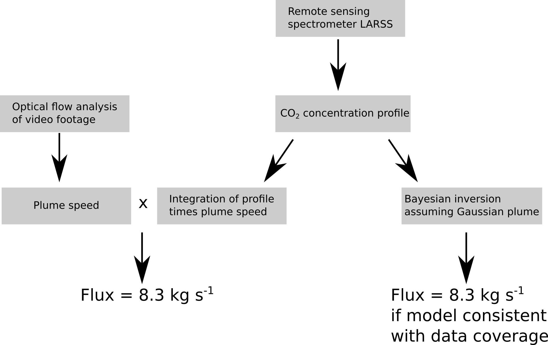
- A direct integration over the scanned area, following Equation (1), using plume speed retrieved from optical flow analysis.
- A Bayesian inversion using a simple Gaussian dispersion forward model.
2. Material and Methods
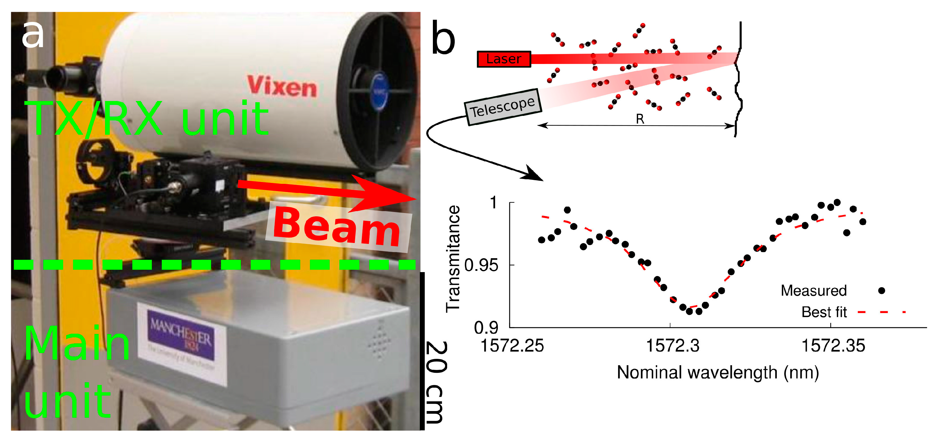
2.1. Remote Sensing of CO2 Concentrations with LARRS
2.2. Flux Retrieval from Direct Integration
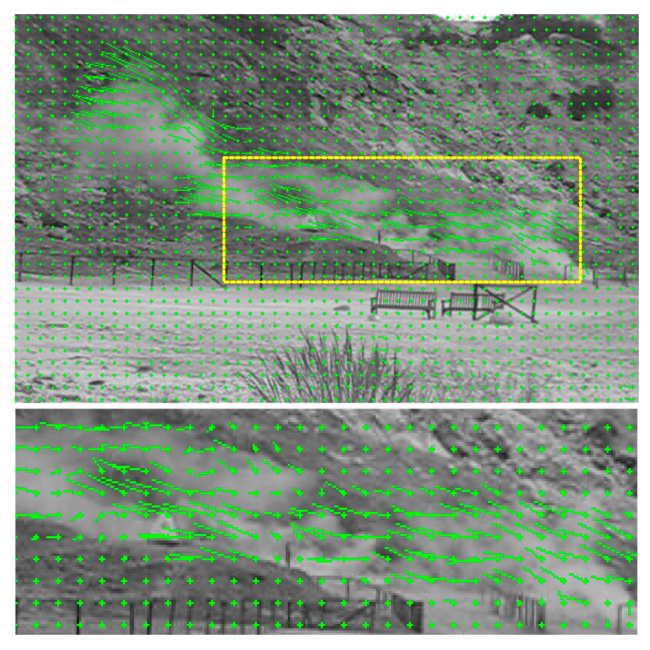
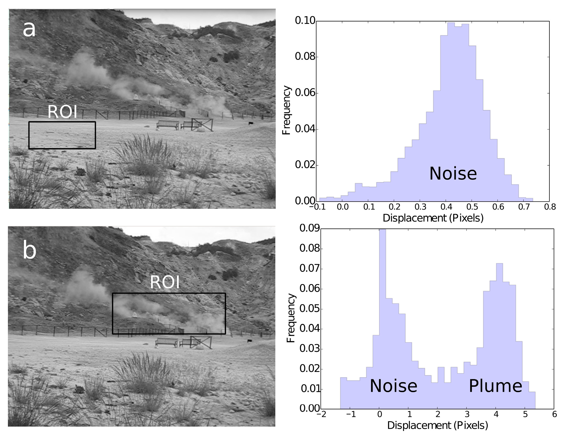
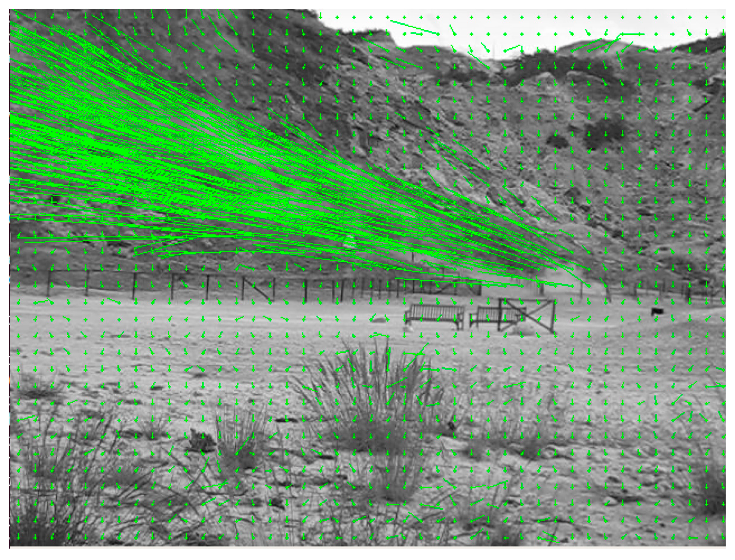
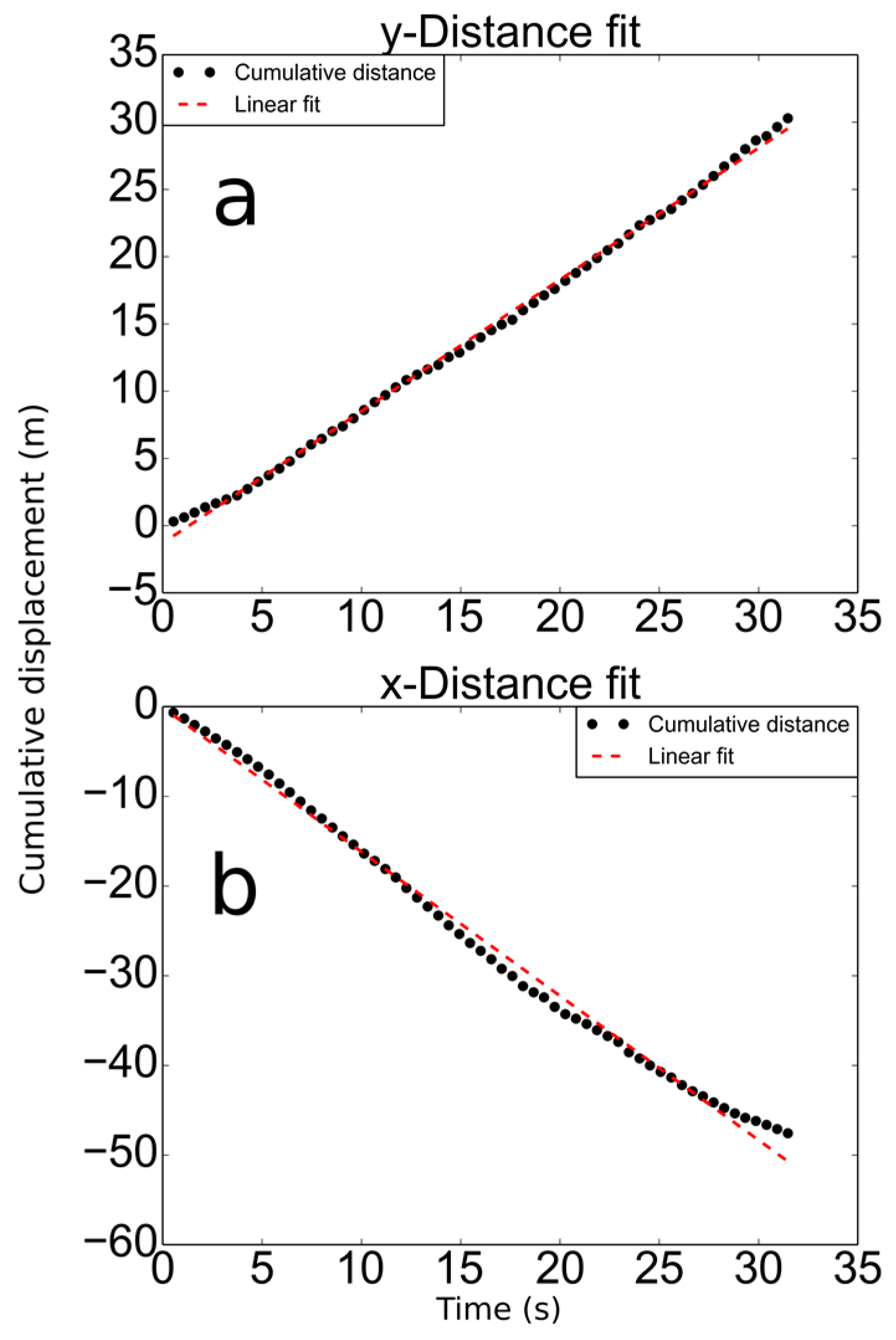
Plume Speed Retrieval Using Optical Flow Analysis
2.3. Flux Retrieval from Bayesian Inversion
3. Field Measurements at Solfatara and the Data
4. Results
4.1. CO2 Flux from Direct Integration
4.2. CO2 Flux from Bayesian Inversion
5. Discussion
5.1. CO2 Flux from Direct Integration
5.2. CO2 Flux from Bayesian Inversion
6. Conclusions
Supplementary Materials
Acknowledgments
Author Contributions
Conflicts of Interest
References
- McGee, K.; Doukas, M.P.; Kessler, R.; Gerlach, T.M. Impacts of Volcanic Gases on Climate, the Environment, and People, U.S. Geological Survey Open-File Report 97-262. Available online: https://pubs.usgs.gov/of/1997/0262/report.pdf (accessed on 5 December 2017).
- Kern, C.; Lübcke, P.; Bobrowski, N.; Campion, R.; Mori, T.; Smekens, J.-F.; Stebel, K.; Tamburello, G.; Burton, M.; Platt, U.; et al. Intercomparison of SO2 camera systems for imaging volcanic gas plumes. J. Volcanol. Geotherm. Res. 2015, 300, 22–36. [Google Scholar] [CrossRef]
- La Spina, A.; Burton, M.R.; Harig, R.; Mure, F.; Rausch, P.; Jordan, M.; Caltabiano, T. New insights into volcanic processes at Stromboli from Cerberus, a remote-controlled open-path FTIR scanner system. J. Volcanol. Geotherm. Res. 2013, 249, 66–76. [Google Scholar] [CrossRef]
- Burton, M.R.; Sawyer, G.M.; Granieri, D. Deep carbon emissions from Volcanoes. Rev. Mineral. Geochem. 2013, 75, 323–354. [Google Scholar] [CrossRef]
- Aiuppa, A.; Fiorani, L.; Santoro, S.; Parracino, S.; Nuvoli, M.; Chiodini, G.; Minopoli, C.; Tamburello, G. New ground-based lidar enables volcanic CO2 flux measurements. Sci. Rep. 2015, 5, 13614. [Google Scholar] [CrossRef] [PubMed]
- Boudoire, G.; Di Muro, A.; Liuzzo, M.; Ferrazzini, V.; Peltier, A.; Gurrieri, S.; Michon, L.; Giudice, G.; Kowalski, P.; Boissier, P. New perspectives on volcano monitoring in a tropical environment: Continuous measurements of soil CO2 flux at Piton de la Fournaise (La Réunion Island, France). Geophys. Res. Lett. 2017, 44, 8244–8253. [Google Scholar] [CrossRef]
- Chiodini, G.; Paonita, A.; Aiuppa, A.; Costa, A.; Caliro, S.; De Martino, P.; Acocella, V.; Vandemeulebrouck, J. Magmas near the critical degassing pressure drive volcanic unrest towards a critical state. Nat. Commun. 2016, 7, 13712. [Google Scholar] [CrossRef] [PubMed]
- De Natale, G.; Troise, C.; Kilburn, C.R.J.; Somma, R.; Moretti, R. Understanding volcanic hazard at the most populated caldera in the world: Campi Flegrei, Southern Italy. Geochem. Geophys. Geosyst. 2017, 18, 2004–2008. [Google Scholar] [CrossRef]
- Chiodini, G.; Frondini, F.; Cardellini, C.; Granieri, D.; Marini, L.; Ventura, G. CO2 degassing and energy release at Solfatara Volcano, Campi Flegrei, Italy. J. Geophys. Res. 2001, 106, 16213–16221. [Google Scholar] [CrossRef]
- Aiuppa, A.; Tamburello, G.; Di Napoli, R.; Cardellini, C.; Chiodini, G.; Giudice, G.; Grassa, F.; Pedone, M. First observations of the fumarolic gas output from a restless caldera: Implications for the current period of unrest (2005–2013) at Campi Flegrei. Geochem. Geophys. Geosyst. 2013, 14, 4153–4169. [Google Scholar] [CrossRef]
- Pedone, M.; Aiuppa, A.; Giudice, G.; Grassa, F.; Cardellini, C.; Chiodini, G.; Valenza, M. Volcanic CO2 flux measurement at Campi Flegrei by Tunable Diode Laser absorption Spectroscopy. Bull. Volcanol. 2014, 76, 812. [Google Scholar] [CrossRef]
- Queißer, M.; Granieri, D.; Burton, M. A new frontier in CO2 flux measurements using a highly portable DIAL laser system. Sci. Rep. 2016, 6, 33834. [Google Scholar] [CrossRef]
- Queißer, M.; Granieri, D.; Burton, M.R.; Arzilli, F.; Avino, R.; Carandente, A. Increasing CO2 flux at Pisciarelli, Campi Flegrei, Italy. Solid Earth 2017, 8, 1017–1024. [Google Scholar] [CrossRef]
- Carapezza, M.L.; Inguaggiato, S.; Brusca, L.; Longo, M. Geochemical precursors of the activity of an open-conduit volcano: The Stromboli 2002–2003 eruptive events. Geophys. Res. Lett. 2004, 31, L07620. [Google Scholar] [CrossRef]
- Giammanco, S.; Parello, F.; Gambardella, B.; Schifano, R.; Pizzullo, S.; Galante, G. Focused and diffuse effluxes of CO2 from mud volcanoes and mofettes south of Mt. Etna (Italy). J. Volcanol. Geotherm. Res. 2007, 165, 46–63. [Google Scholar] [CrossRef]
- Amediek, A.; Fix, A.; Wirth, M.; Ehret, G. Development of an OPO system at 1.57 µm for integrated path DIAL measurement of atmospheric carbon dioxide. Appl. Phys. B 2008, 92, 295–302. [Google Scholar] [CrossRef]
- Kameyama, S.; Imaki, M.; Hirano, Y.; Ueno, S.; Kawakami, S.; Sakaizawa, D.; Kimura, T.; Nakajima, M. Feasibility study on 1.6 μm continuous-wave modulation laser absorption spectrometer system for measurement of global CO2 concentration from a satellite. Appl. Opt. 2011, 50, 2055–2068. [Google Scholar] [CrossRef] [PubMed]
- Thomas, B.; David, G.; Anselmo, C.; Cariou, J.-P.; Miffre, A.; Rairoux, P. Remote sensing of atmospheric gases with optical correlation spectroscopy and lidar: First experimental results on water vapor profile measurements. Appl. Phys. B 2013, 113, 265–275. [Google Scholar] [CrossRef]
- Shibata, Y.; Nagasawa, C.; Makoto, A. Development of 1.6 μm DIAL using an OPG/OPA transmitter for measuring atmospheric CO2 concentration profiles. Appl. Opt. 2017, 56, 1194–1201. [Google Scholar] [CrossRef] [PubMed]
- Feitz, A. (Geoscience Australia, Canberra, Australia). Personal communication, 2017.
- Flesch, T.K.; Wilson, J.D.; Harper, L.H.; Crenna, B.P. Estimating gas emissions from a farm with an inverse-dispersion technique. Atmos. Environ. 2005, 39, 4863–4874. [Google Scholar] [CrossRef]
- Kuske, T.; Jenkins, C.; Zegelina, S.; Mollahe, M.; Feitz, A. Atmospheric tomography as a tool for quantification of CO2 emissions from potential surface leaks: Signal processing workflow for a low accuracy sensor array. Energy Proc. 2013, 37, 4065–4076. [Google Scholar] [CrossRef]
- Largeron, Y.; Guichard, F.; Bouniol, D.; Couvreux, F.; Kergoat, L.; Marticorena, B. Can we use surface wind fields from meteorological reanalyses for Sahelian dust emission simulations? Geophys. Res. Lett. 2015, 42, 2490–2499. [Google Scholar] [CrossRef]
- Wanninkhof, R. Relationship between wind speed and gas exchange over the ocean revisited. Limnol. Oceanogr. Methods 2014, 12, 351–362. [Google Scholar] [CrossRef]
- Wu, F.; Li, A.; Xie, P.; Chen, C.; Hu, Z.; Zhang, Q.; Liu, J.; Liu, W. Emission Flux Measurement Error with a Mobile DOAS System and Application to NOx Flux Observations. Sensors 2017, 17, 231. [Google Scholar] [CrossRef] [PubMed]
- Fiorani, L. Lidar application to lithosphere, hydrosphere and atmosphere. In Progress in Laser and Electro-Optics Research; Koslovskiy, V.V., Ed.; Nova: New York, NY, USA, 2010; pp. 21–75. [Google Scholar]
- Bouquet, M.; Parmentier, R.; Sauvage, L.; Cariou, J.-P. Theoretical and CFD Analysis of Pulsed Doppler Lidar Wind Profile Measurement Process in Complex Terrain. In Proceedings of the EWEA European Wind Energy Conference, Warsaw, Poland, 20–23 April 2010. [Google Scholar]
- Lang, S.; McKeogh, E. LIDAR and SODAR Measurements of Wind Speed and Direction in Upland Terrain for Wind Energy Purposes. Remote Sens. 2011, 3, 1871–1901. [Google Scholar] [CrossRef]
- Weibring, P.; Andersson, M.; Edner, H.; Svanberg, S. Remote monitoring of industrial emissions by combination of lidar and plume velocity measurements. Appl. Phys. B 1998, 66, 383–388. [Google Scholar] [CrossRef]
- Mori, T.; Burton, M. Quantification of the gas mass emitted during single explosions on Stromboli with the SO2 imaging camera. J. Volcanol. Geotherm. Res. 2009, 188, 395–400. [Google Scholar] [CrossRef]
- Queißer, M.; Burton, M.R.; Arzilli, F.; Chiarugi, A.; Marliyani, G.I.; Anggara, F.; Harijoko, A. CO2 flux from Javanese mud volcanism. J. Geophys. Res. Solid Earth 2017, 122, 4191–4207. [Google Scholar] [CrossRef] [PubMed]
- Peters, N.; Hoffmann, A.; Barnie, T.; Herzog, M.; Oppenheimer, C. Use of motion estimation algorithms for improved flux measurements using SO2 cameras. J. Volcanol. Geotherm. Res. 2015, 300, 58–69. [Google Scholar] [CrossRef]
- Santoro, S.; Parracino, S.; Fiorani, L.; D’Aleo, R.; Di Ferdinando, E.; Giudice, G.; Maio, G.; Nuvoli, M.; Aiuppa, A. Volcanic Plume CO2 Flux Measurements at Mount Etna by Mobile Differential Absorption Lidar. Geosciences 2017, 7, 9. [Google Scholar] [CrossRef]
- Klein, A.; Lübcke, P.; Bobrowski, N.; Kuhn, J.; Platt, U. Plume propagation direction determination with SO2 cameras. Atmos. Meas. Tech. 2017, 10, 979–987. [Google Scholar] [CrossRef]
- Gliß, J.; Stebel, K.; Kylling, A.; Sudbø, A. Optical flow gas velocity analysis in plumes using UV cameras—Implications for SO2-emission-rate retrievals investigated at Mt. Etna, Italy, and Guallatiri, Chile. Atmos. Meas. Tech. Discuss. 2017. in review. [Google Scholar] [CrossRef]
- Farnebäck, G. Two-Frame Motion Estimation Based on Polynomial Expansion. In Heidelberg Image Analysis; SCIA 2003, Lecture Notes in Computer Science; Bigun, J., Gustavsson, T., Eds.; Springer: Berlin, Germany, 2003; Volume 2749. [Google Scholar]
- Sangeeta, B.; Feitz, A.; Francis, A. Atmospheric Tomography, GitHub Repository. Available online: https://github.com/GeoscienceAustralia/atmospheric_tomography_laser (accessed on 15 November 2017).
- Granieri, D.; Costa, A.; Macedonio, G.; Bisson, M.; Chiodini, G. Carbon dioxide in the urban area of Naples: Contribution and effects of the volcanic source. J. Volcanol. Geotherm. Res. 2013, 260, 52–61. [Google Scholar] [CrossRef]
- Schmidt, A.; Rella, C.W.; Göckede, M.; Hanson, C.; Yang, Z.; Law, B.E. Removing traffic emissions from CO2 time series measured at a tall tower using mobile measurements and transport modeling. Atmos. Environ. 2014, 97, 94–108. [Google Scholar] [CrossRef]
- INGV: Bollettino di Sorgevlianza Campi Flegrei October 2017. Available online: http://www.ov.ingv.it/ov/bollettini-mensili-campania/Bollettino%20Mensile%20Campi%20Flegrei%202017_04.pdf (accessed on 30 November 2017).
- Pedone, M.; Granieri, D.; Moretti, R.; Fedele, A.; Troise, C.; Somma, R.; De Natale, G. Improved quantification of CO2 emission at Campi Flegrei by combined Lagrangian Stochastic and Eulerian dispersion modelling. Atmos. Environ. 2017, 170, 1–11. [Google Scholar] [CrossRef]
- Humphries, R.; Jenkins, C.; Leuning, R.; Zegelin, S.; Griffith, D.; Caldow, C.; Berko, H.; Feitz, A. Atmospheric Tomography: A Bayesian Inversion Technique for Determining the Rate and Location of Fugitive Emissions. Environ. Sci. Technol. 2012, 46, 1739–1746. [Google Scholar] [CrossRef] [PubMed]


| (°) | (m s−1) | (°C) | (%) | (hPa) |
|---|---|---|---|---|
| 210 | 1.4 | 18.0 | 75 | 1005 |
| Input Parameter | Value or Source |
|---|---|
| In-plume CO2 mixing ratios | Equation (4) |
| Instrument location | UTM 427556 4520015 |
| Target location | Derived from angle and length of rays (Figure 1b) |
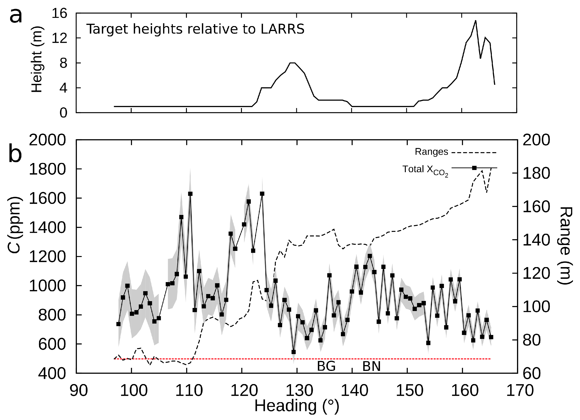
| Target height | Figure 5a |
| Vent height | 1 m |
| Air temperature | 18 °C (Table 1) |
| Air pressure | 100,500 Pa (Table 1) |
| Wind speed | 1.4 m s−1 (Table 1) |
| Wind direction | 210° (Table 2) |
| Monin–Obhukov length | −5.5 m |
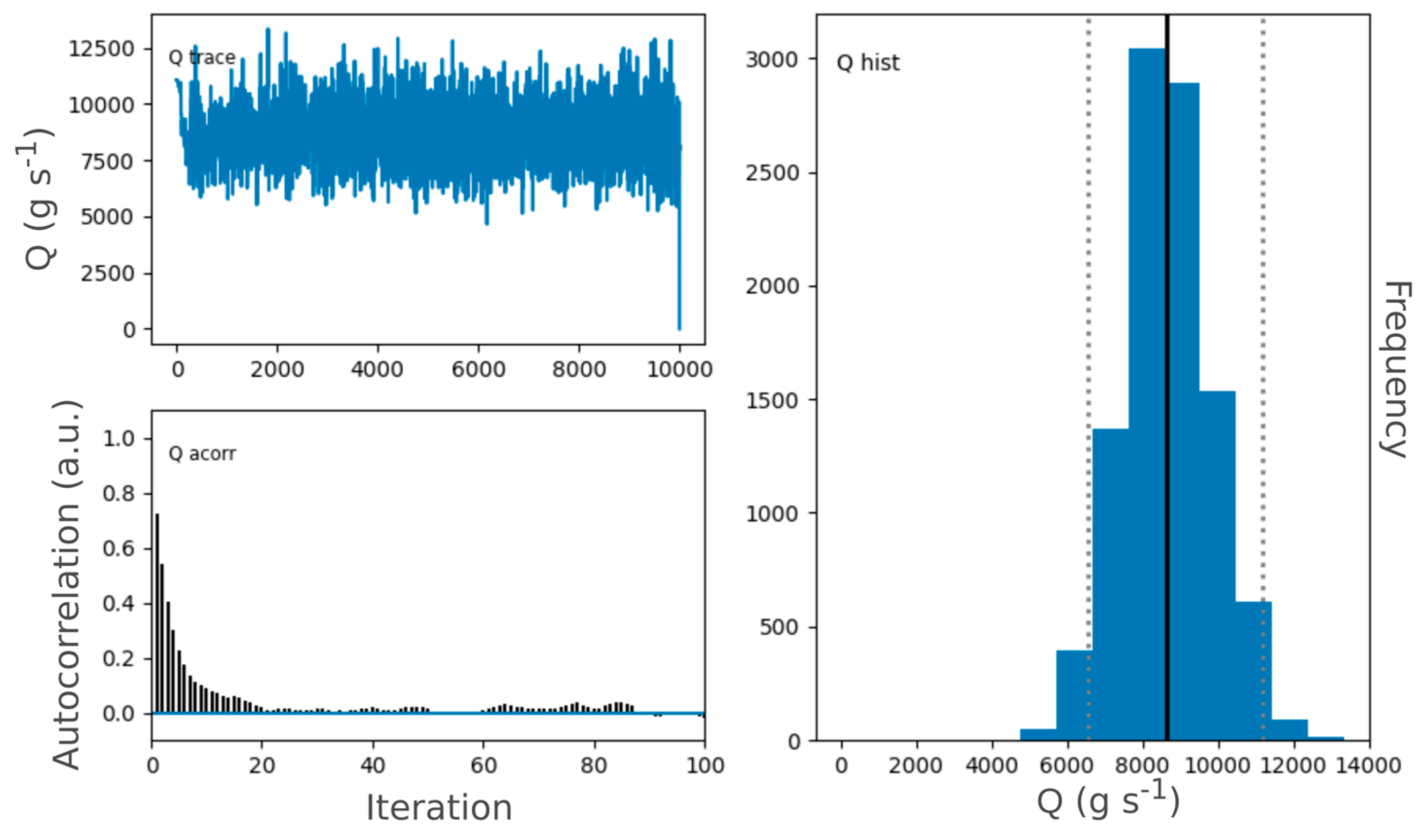
| Number of MCMC iterations | 30,000 |
| Thinning parameter | 3 |
© 2018 by the authors. Licensee MDPI, Basel, Switzerland. This article is an open access article distributed under the terms and conditions of the Creative Commons Attribution (CC BY) license (http://creativecommons.org/licenses/by/4.0/).
Share and Cite
Queißer, M.; Burton, M.; Granieri, D.; Varnam, M. Ground-Based Remote Sensing of Volcanic CO2 Fluxes at Solfatara (Italy)—Direct Versus Inverse Bayesian Retrieval. Remote Sens. 2018, 10, 125. https://doi.org/10.3390/rs10010125
Queißer M, Burton M, Granieri D, Varnam M. Ground-Based Remote Sensing of Volcanic CO2 Fluxes at Solfatara (Italy)—Direct Versus Inverse Bayesian Retrieval. Remote Sensing. 2018; 10(1):125. https://doi.org/10.3390/rs10010125
Chicago/Turabian StyleQueißer, Manuel, Mike Burton, Domenico Granieri, and Matthew Varnam. 2018. "Ground-Based Remote Sensing of Volcanic CO2 Fluxes at Solfatara (Italy)—Direct Versus Inverse Bayesian Retrieval" Remote Sensing 10, no. 1: 125. https://doi.org/10.3390/rs10010125
APA StyleQueißer, M., Burton, M., Granieri, D., & Varnam, M. (2018). Ground-Based Remote Sensing of Volcanic CO2 Fluxes at Solfatara (Italy)—Direct Versus Inverse Bayesian Retrieval. Remote Sensing, 10(1), 125. https://doi.org/10.3390/rs10010125