Article

Improving the Accuracy of Land Use and Land Cover Classification of Landsat Data Using Post-Classification Enhancement

Faculty of Agriculture, Food and Natural Resources, The University of Sydney, Sydney, NSW 2006, Australia
*
Author to whom correspondence should be addressed.
Remote Sens. 2009, 1(3), 330-344; https://doi.org/10.3390/rs1030330
Submission received: 2 July 2009 / Revised: 14 July 2009 / Accepted: 23 July 2009 / Published: 31 July 2009

Abstract

:
Classifying remote sensing imageries to obtain reliable and accurate land use and land cover (LULC) information still remains a challenge that depends on many factors such as complexity of landscape, the remote sensing data selected, image processing and classification methods, etc. The aim of this paper is to extract reliable LULC information from Landsat imageries of the Lower Hunter region of New South Wales, Australia. The classical maximum likelihood classifier (MLC) was first applied to classify Landsat-MSS of 1985 and Landsat-TM of 1995 and 2005. The major LULC identified were Woodland, Pasture/scrubland, Vineyard, Built-up and Water-body. By applying post-classification correction (PCC) using ancillary data and knowledge-based logic rules the overall classification accuracy was improved from about 72% to 91% for 1985 map, 76% to 90% for 1995 map and 79% to 87% for 2005 map. The improved overall Kappa statistics due to PCC were 0.88 for the 1985 map, 0.86 for 1995 and 0.83 for 2005. The PCC maps, assessed by McNemar’s test, were found to have much higher accuracy in comparison to their counterpart MLC maps. The overall improvement in classification accuracy of the LULC maps is significant in terms of their potential use for land change modelling of the region.

Graphical Abstract

1. Introduction

Change in land use and land cover (LULC) is gaining recognition as a key driver of environmental changes [1,2]. Preserving the environmental resources while maintaining or enhancing the economic and social benefits from their use is a present day challenge. For this reason, there is a need to understand the pattern and trends of LULC changes on the local, regional and global scales. Advances in remote sensing science and associated technologies have made it possible to obtain valuable spatiotemporal information on LULC. The search for methods used for producing accurate LULC and determining LULC change over time has been an important component of remote sensing research within the last two decades or so. However, classifying a remote sensing imagery still remains a challenge that depends on many factors such as complexity of landscape in a study area, the choice of remote sensing data, and image processing and classification approaches etc [3,4]. Quite often, LULC maps derived from remote sensing are judged insufficient in quality and, thus not trustworthy for quantitative environmental application purposes [5,6,7]. This has led to questioning of the spectral and radiometric suitability of remotely sensed data sets for thematic mapping. This means that specific types of change must be identified using aerial photography and ground reconnaissance [5]. Wilkinson [7], based on a review of 15 years of peer-reviewed experiments on satellite image classification, observed that there has been no demonstrable improvement in classification performance over this 15-year period although a considerable inventiveness had occurred in establishing and testing new classification methods during the period [7]. This raises some doubts about the value of continued research efforts to improve classification algorithms in remote sensing. Jensen [8] opined that low reliability of remote sensing classification is not surprising because 95% of the scientists attempt to accomplish classification only using one variable i.e., spectral characteristic (colour) or black and white tone. However, other researchers have utilised ancillary data in combination with remote sensing data to improve classification accuracy [9,10,11,12,13,14]. This study is therefore built on the premise that the use of ancillary data combined with spectral and contextual knowledge will improve the overall accuracy of LULC classification.
Landsat TM/ETM+ spectral data are frequently used for LULC classification on regional scales [4,9,12,14,15] due to their relatively lower cost, longer history and higher frequency of archives. This is more important because information regarding the LULC over time and space is a fundamental requirement for environmental monitoring in order to prevent detrimental environmental impacts before they become irreparable. In this study, the Landsat TM data were classified with the most widely used parametric classifier, maximum likelihood decision rule and some ancillary data (e.g., DEM and knowledge of the locality, Land use data, vegetation index and textural analysis of the Landsat images) were combined through an expert (or hypothesis testing) system to improve the classification accuracy so that these classified maps could be used for detailed post-classification change detection. The aim of this paper was therefore to assess the hypothesis that the use of ancillary data could lead to improvement of land use classification. This aim is particularly pertinent because good quality satellite imageries of the study region for specific periods of interest to us were not available due to cloud cover and atmospheric haziness-common phenomena in the study region.

2. Study Area

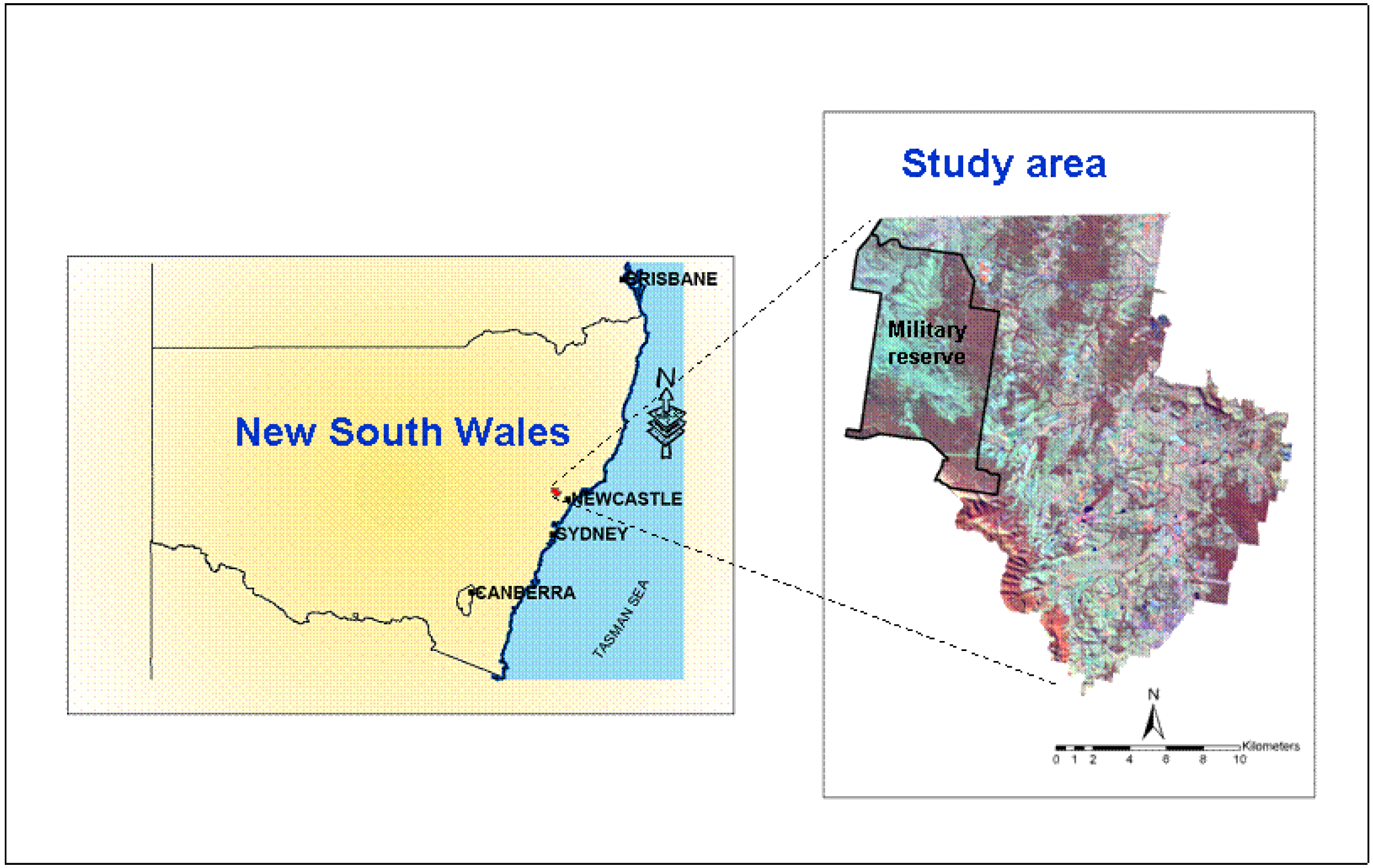
The study area, generally referred to as the ‘Hunter Wine Country Private Irrigation District’ (HWCPID), is located in the Lower Hunter region of New South Wales (NSW) Australia, about 160 km north of Sydney (Figure 1). The region currently contains the sixth largest urban area in Australia with diverse land uses and landscapes, the latter consisting of coastline, mountains, lakes, floodplains and a river and also includes the world’s largest coal exporting port. Mining and industrial manufacturing have been the source of the strong economic activity of the region [16]. The regional planning strategy was focused on provision of sufficient new urban development and employment to meet expected strong demand for growth in population from 515,000 persons in 2006 to an estimated 675,000 persons by 2031 [16]. A substantial proportion of this increase in population is expected to be settled in the HWCPID. The HWCPID, covering an approximately 379 km2, is located within an undulating plain of the Lower Hunter valley, centred on the little town of Pokolbin. Geographically it lies between 151°09'43" E to 151°24'58" E Longitude and 32°37'21" S to 32°51'45" S Latitude. In HWCPID land use ranges from viticulture and dairying to extensive grazing and forestry. Pastoral systems were the dominant agricultural land use in the region for past 100 years, while grape vines were introduced in the 1820s. However, the expansion of vineyards to their present level started in the latter half of the 20th century. Other land uses include livestock production for beef, and vegetable production. In order to protect the booming grape vine cultivation from drought, Pokolbin Pipeline Project (PPP) was established in 2000. The network was designed to supply water to nearly 400 properties spread throughout the project area (Ken Bray, personal communication, 2008).
Figure 1. Location of study area (HWCPID) in New South Wales as a Landsat TM image of 2005 (in RGB combination of bands 4, 3 and 5).
Remotesensing 01 00330 g001
The area has been gaining popularity as a tourist attraction due to the presence of numerous wineries, stretching grape vineyard beyond the horizon, and golf courses. However, Pokolbin’s image of a bucolic rural landscape with its varied mosaic of vineyards, pastures, scattered woodlands and wineries, has been threatened by the prospects of overdevelopment [17]. This creates concerns among the public, and has evoked the inevitable tradeoffs between development, economic growth and environmental quality.

3. Methods

3.1. Landsat, Ancillary and Reference Data

For the purpose of this study the orthocorrected Landsat images of following were procured: Landsat 5-MSS of January 8, 1985, Landsat 5-TM of August 6, 1995, and Landsat 5-TM of June 8, 2005. The study area is contained within the Landsat path 89, row 83. All images were re-projected to the new Australian Geodetic Datum GDA-1994 and were all re-sampled to a common nominal spatial grid of 25 m resolution using nearest neighbour technique. This was to facilitate the operations that would be required for the change detection analysis. The root mean square errors of re-sampling and re-projection of the images were less than 0.5 pixel, equivalent to approximately 7–15 m.
High resolution orthorectified aerial photographs acquired sometime between 2004 and 2006 were also procured from Plateau Images, Alstonville, New South Wales. Additionally, the following data were procured: black and white aerial photographs acquired in 1984, colour aerial photographs acquired in 1991 and 1998 (all from Department of Land, NSW Govt.), and the Singleton Land use geodatabase (currency 2000-2007) and digital elevation model (DEM) (from Department of Natural Resources, NSW Govt.). The aerial photographs were orthorectified using the above mentioned orthorectified aerial photographs (years 2004 to 2006). The aerial photographs for each time period were mosaicked as one image for convenience of projection. The resolutions of these aerial photographs were 2 m. The aerial photographs were mainly used as reference data and the Singleton Land use geodatabase and DEM were utilized as ancillary data for post-classification correction using knowledge base.
Table 1. LULC categories delineated for the classification.
LULC categoryDescription
WoodlandForest covers including tree cover along the creeks
Pasture/scrublandNatural and cultivated pastures, and scrubs with partial grassland
VineyardIrrigated and non irrigated vineyards
Built-upCommercial, and residential areas, and other areas with man-made structure; roads, railway lines
Water-bodyFarm dams, sewage ponds
Mine/quarryMining areas
OliveOlive plantations (for 2005 only)

3.2. LULC Classification Based on Maximum Likelihood Classifier

Maximum likelihood classifier (MLC) is the most widely adopted parametric classification algorithm [8,11,18,19,20]. For this reason we used MLC for the spectral classification of the Landsat images. Taking into account the spectral characteristics of the satellite images and existing knowledge of land use of the study area, six LULC categories (Table 1) were respectively identified and classified for 1985 and 1995 and seven for 2005, as the Olive category did not exist prior to 1995. Though this category covered only a small proportion of the region, we delineated it due to its expansion in recent years.
Jensen [8] has opined that the derivation of the level II classes of US Geological Survey Land-use Land-Cover Classification System, using Landsat TM data, is inappropriate due to the limitations imposed by the medium spatial resolution and the difficulty in interpretability. The same limitations were applicable in this study as Pasture/scrubland and Vineyard could not be separated into irrigated and non-irrigated ones, due to their noisy Landsat spectral signatures and difficulty in interpreting them. Of the two Landsat TM images used, one thermal band (band 6) was excluded prior to MLC classification. However, in the case of Landsat MSS image, all the four bands were used for classification. The aerial photograph corresponding to each year was used to identify the “true” LULC parcels on the ground used for training. In cases where a single pre-defined LULC category has a different spectral signature in different areas, multiple signatures were created, but were later merged into one signature for a given LULC category. We performed an evaluation of collected signatures through exploratory analysis of histogram, contingency matrix and computing signature separability using a given transformed divergence for a distance between signatures. Signatures were recollected if not producing satisfactory results. In the case of Water LULC category, signature was collected from a feature space of 2-5 band combination (non-parametric rule). Thresholding was also done which is the process of identifying the pixels in a classified image that are the most likely to be classified incorrectly [21]. The distance image and output thematic raster layer produced by MLC were used for thresholding. The tails of histograms (pixels that are most likely to be misclassified have the higher distance file values at the tail of the histogram of the distance image) were cut off interactively and saved and the removed pixels were viewed. Consequently there were only a few small speckles of the removed pixels. Once the collected signatures were comparatively satisfactory, multiple signatures were merged into one signature for a given LULC category and used for the classification.

3.3. Post-Classification Refinement Using Ancillary Data and Logic Rule

As the LULC maps were noisy due to similarities of the spectral responses of certain land cover categories such as Pasture/scrubland, Vineyard and Built-up (as discussed in section 4.1 below), a post-classification refinement was developed and applied using ancillary information using a hypothesis testing framework of Knowledge Engineer [21] to reduce classification errors. The hypothesis framework was constructed by using the Singleton land use map, DEM, textural analysis and NDVI (Normalized Difference Vegetation Index) derived from the Landsat images. The framework was further augmented by the use of the orthorectified aerial photographs. Through this framework the misclassified pixels of MLC were re-evaluated and correctly reclassified. The different post-classification procedures adopted for the mix-classified LULC categories, namely, Built-up and Vineyard, are described as follows.

3.3.1. Built-up post-classification correction
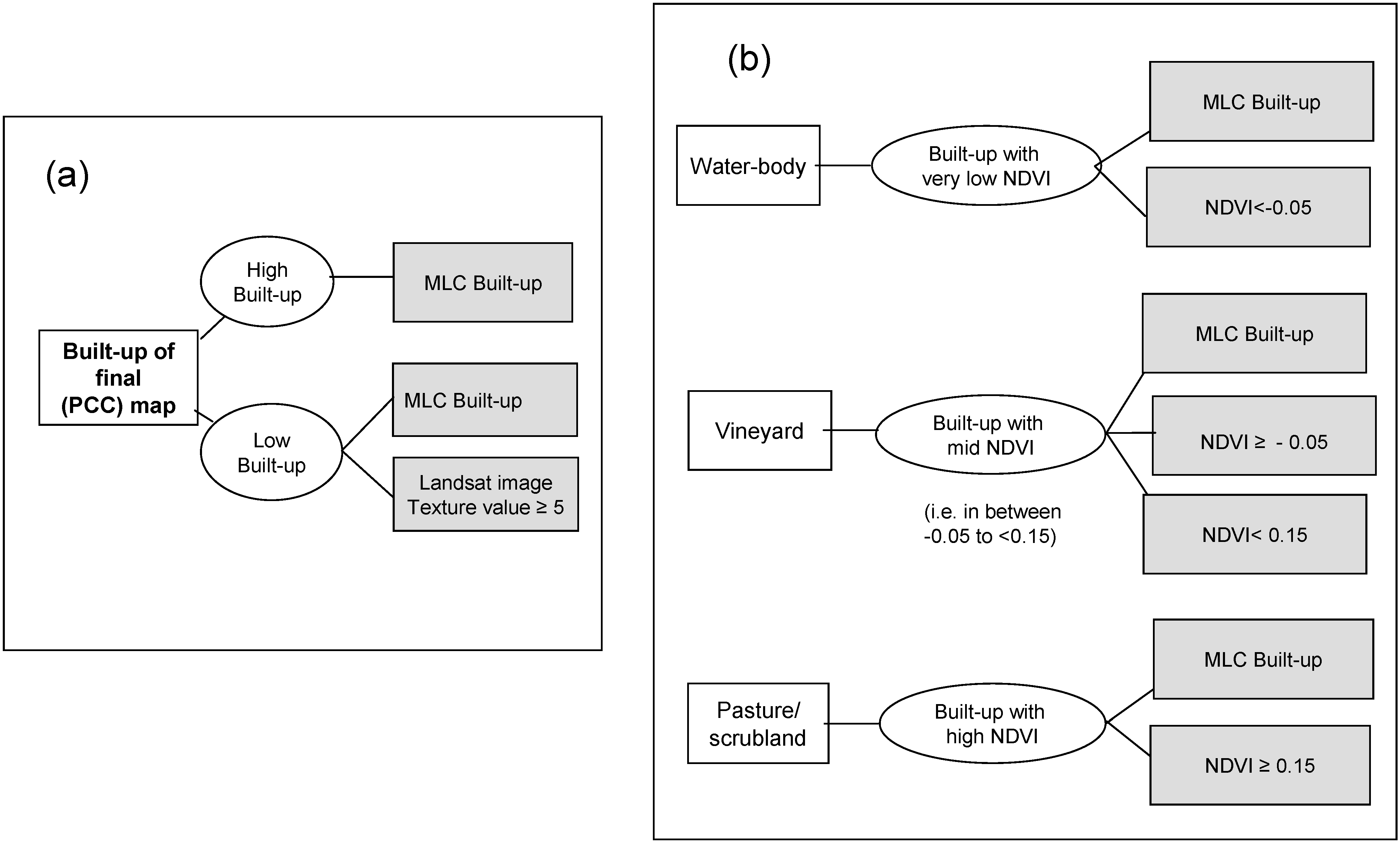
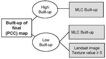
The Built-up LULC patches under Landsat images were generally characterized by high textural value resulting from variegation caused by different features such as buildings, street grids and urban corridors. This is in contrast to the homogenous Pastures which have little to no textural variation. In this study, the MLC maps had high commission error especially in low built-up areas. For this reason, a modified textural analysis [9] was used. However, in our case, the correction based on textural analysis was only applied for the low-built-up areas to avoid increasing the omission error. For this, an AOI (area of interest) was drawn around the high-built-up area, and using the logic rule shown in Figure 2, all Built-up pixels of MLC were retained as such in the post-classification corrected (PCC) map. The MLC Built-up patches in the rest of the study area were modified using the following logic rules: the Built-up pixels of MLC classification with texture value above some critical level (it was ≥5 for 1985 and 2005 Landsat images, and ≥20 in the case of 1995 images) are retained as new Built-up pixels (Figure 2a). The remainder of the MLC Built-up patches were reclassified based on their NDVI threshold values, for example, if NDVI is less than -0.05, then allocated it to Water-body, and if the NDVI value is between -0.05 and 0.15, then reclassified to Vineyard, otherwise to Pasture/scrubland (Figure 2b). These threshold values were determined by detailed inspection of the textural images and NDVI images derived from the respective Landsat imageries corresponding to the LULC categories of interest which was guided with the use of orthorectified aerial photograph of the nearby period.
Figure 2. Hypothesis testing framework for Built-up correction. In both (a) and (b): the left white box is the hypothesis being tested, the ellipses represent the conjunctive decision rules and right shaded boxes represent the variables used. (a) Built-up of MLC classification with the Landsat textural value above some critical level only is retained as Built-up of PCC classification in case of low Built-up areas. (b) Built-up of MLC classification which is not included as Built-up of PCC classification are reclassified to other LULC categories based on critical levels of NDVI values.
Remotesensing 01 00330 g002
The texture analysis [21] of the TM band was performed using a 3 × 3 moving window and the variance Equation (1):
V = ( x i j M ) 2 n 1
where xij = DN value of pixel (i, j); n = number of pixels in a window; and M is the mean of the moving window which is defined in Equation (2):
M = x i j n
Normalized Difference Vegetation Index (NDVI) is the most widely used vegetation index to distinguish healthy vegetation from others or from non-vegetated areas. NDVI was derived using the expression given in Equation (3):
N D V I = ( N I R R ) ( N I R + R )
where NIR = Near Infra Red (band 4 for both Landsat TM and Landsat MSS); R = Red (band 3 in case of Landsat TM images and band 2 for Landsat MSS).

3.3.2. Vineyard post-classification correction

The identification of Vineyards by the satellite sensor is made difficult because they are characterised by bare ground or pasture-like feature between the vine rows, leading to high spectral similarity with the bare ground, scanty grasses in the military reserve (Figure 1) in the north-west and the rocky open woodland to the west. Therefore, the initially misclassified Vineyard pixels in the military reserve were reclassified into Pasture/scrubland, and the apparent Vineyard pixels among the Woodland in the western part of the study area were reclassified into Woodland using a hypothesis testing logic rule. For this, the military reserve and state forest boundaries of the Singleton land use map were utilized for reclassifying the pixels. Additionally, as Vineyard was not expected to be found on elevations higher than 250 m, the misclassified Vineyard pixels above this elevation were also reclassified as Pasture/scrubland. This approach largely corrected the Vineyard and Pasture/scrubland areas. However some further minor corrections were done based on the interpretation of aerial photos and field validation through visits to the study area and personal communication with the local people.

3.3.3. Other minor post-classification corrections

Apart from the Built-up and Vineyard LULC categories, some corrections were made on the Mine/quarry LULC category. The apparent Built-up and Vineyard classified in the real mining patches were converted to Mine/quarry (by using AOI of the area and with a logic rule). Similarly for the 2005 MLC LULC map, the apparent Olive Farms identified at high elevation to the west of the study area were converted to Woodland as olive farms were not expected in state forest areas. Finally the road and railway networks (derived from the Singleton land use map) were added to the Built-up category. The major transport infrastructure had been developed in the area long before 1980s, which was confirmed using historical aerial photographs.

3.4. Accuracy Assessment

The users of LULC maps need to know how accurate the maps are in order to use the data more correctly and efficiently [22,23]. According to Anderson et al. [24], the minimum level of interpretation accuracy in the identification of land use and LULC categories from remote sensing data should be at least 85%. The most widely promoted classification accuracy is in the form of error matrix which can be used to derive a series of descriptive and analytical statistics [6,22,25,26,27]. The procedure is a very effective way to represent accuracy in that the accuracies of each category are plainly described along with both the errors of inclusion (commission errors) and errors of exclusion (omission errors) present in the classification [25]. Overall accuracy, producer’s accuracy, user’s accuracy and Kappa statistics are generally reported, and these terms have been explained in detail in many studies [6,19,22,23,25,26,27,28].
In this study, accuracy assessment was performed for the MLC and PCC classified maps of all three time steps: 1985, 1995, and 2005. Stratified random sampling design was adopted for the accuracy assessment. Only five categories, Woodland, Pasture/scrubland, Vineyard, Built-up, and Water-body were considered for accuracy assessment with the minimum of 50 sample points for each considered category, as recommended by Congalton [25]. The other two LULC categories–Mine/quarry, and Olive- were not considered for accuracy assessment as they cover only a small proportion of the study area. Interpretation is based on aerial photographs and field verification. Overall accuracy, user’s and producer’s accuracies, and the Kappa statistics were derived from the error matrices to find the reliability and accuracy of the maps produced.

3.5. Comparing Classifier Performance

The z-test based on Kappa coefficients is commonly used to infer the superiority of one map production over another. However, this may not be appropriate if the same sample of sites is used in the comparison [29,30,31], as these coefficients assume that the samples used in their calculations are independent. We have used the same set of reference points for testing the accuracy of maps produced by MLC and PCC methods for the same year, to avoid the difference of accuracy due to sampling variability. For this reason, we have performed McNemar’s test [30] to evaluate the superiority of the LULC maps resulting from post-classification over the MLC classified maps. The McNemar’s test is preferable because it is parametric, very simple to understand and execute. Additionally it is more precise and sensitive than the Kappa z-test. The test is based on a chi-square (χ2) statistics, computed from two error matrices using Equation (4):
χ 2 = ( f 12 f 21 ) 2 f 12 + f 21
where f12 denotes number of cases that are wrongly classified by classifier 1 but correctly classified by classifier 2, and f21 denotes number of cases that are correctly classified by classifier 1 but wrongly classified by classifier 2.

4. Results and Discussion

4.1. Classification Accuracy Assessment Using Error Matrices

As would be expected classification using the classical MLC algorithm did not produce satisfactory results especially in the case of Built-up and Vineyard LULC categories. Table 2 shows the mean DN (digital number) values of training pixels of the various LULC categories over band 1–5 and band 7. The difficulty with these signatures is that the mean DN among the LULC categories are quite similar for bands 1 to 3, while there is significant difference among the LULC categories for bands 4, 5 and 7. Pasture/scrubland, Vineyard have relatively larger DN for band 5 followed by Built-up, while Water-body has distinctly lower DN for bands 4, 5 and 7.
Table 2. The mean DN values of the training pixels of different LULC categories used for the maximum likelihood classification; values in bracket are the standard deviations.
LULC categoryBand 1Band 2Band 3Band 4Band 5Band 7
Woodland36.4 (1.3)13.4 (1.1)11.2 (1.6)34.2 (7.4)25.4 (6.9)8.5 (2.5)
Pasture/scrubland43.8 (1.5)19.2 (0.9)22.1 (1.8)32.2 (4.4)58.0 (5.0)24.4 (3.5)
Vineyard43.1 (2.7)18.8 (2.2)21.4 (3.9)27.1 (7.3)54.4 (8.9)27.6 (5.9)
Built-up47.9 (4.5)20.7 (2.4)21.6 (3.7)30.6 (4.3)39.2 (6.6)20.5 (4.6)
Water-body38.3 (1.6)14.6 (1.7)11.9 (2.2)7.2 (2.0)7.0 (2.2)3.8 (1.3)
Mine/quarry43.1 (1.2)16.7 (0.9)16.3 (1.1)13.8 (2.3)20.1 (3.2)11.5 (1.0)
Olive39.4 (0.8)15.9 (0.6)16.0 (0.6)37.3 (1.2)38.3 (1.0)13.5 (0.6)
The poor performance of the MLC classification algorithm is confirmed by the accuracy assessment, which indicated high commission error (i.e., low user’s accuracy) for the Built-up and Vineyard categories, meaning that there is a probability (proportionate to the error) that pixels classified as Built-up and Vineyard may not actually exist on the ground (Table 3). On the other hand, Pasture/scrubland category had high omission error (i.e., low producer’s accuracy), meaning that there is a probability (proportionate to the errors) that ground reference points for this category were classified incorrectly. Lu et al. [32] also found that most of the time, the traditional approach to classification (such as MLC) only distinguishes clearly between forest and non-forest land use and land covers. Similar findings were recorded in this study. The MLC classification accuracy for Woodland and Water body was found to be good, while for other LULC categories the MLC performed quite poorly. As Vineyard paddocks are either characterised by bare ground or alternate pasture between the rows of grape crops, the spectral signatures resembled that of scanty vegetation of Pasture/scrubland, more so in the military reserve and rocky outcrops of the mountainous State Forest to the west. Additionally, the Built-up category also was overestimated.
Table 3. Summary of Accuracy (%) and Kappa statistics of MLC and PCC maps.
LULC category1985 Accuracy1995 Accuracy2005 Accuracy
Producer’sUser’sProducer’sUser’sProducer’sUser’s
MLC maps
Woodland85.193.490.796.383.291.8
Pasture/scrubland47.990.055.496.765.090.3
Vineyard81.544.089.352.687.762.5
Built-up93.255.696.051.195.756.3
Water-body98.0100.083.3100.088.996.0
Overall accuracy71.876.3 79.3
Kappa statistics0.640.700.74
PCC maps
Woodland98.5100.094.291.088.889.6
Pasture/scrubland81.798.688.590.981.188.6
Vineyard98.271.692.977.687.773.5
Built-up98.382.980.088.991.582.7
Water-body98.010090.098.290.796.1
Overall accuracy91.389.586.6
Kappa statistics0.880.86 0.83
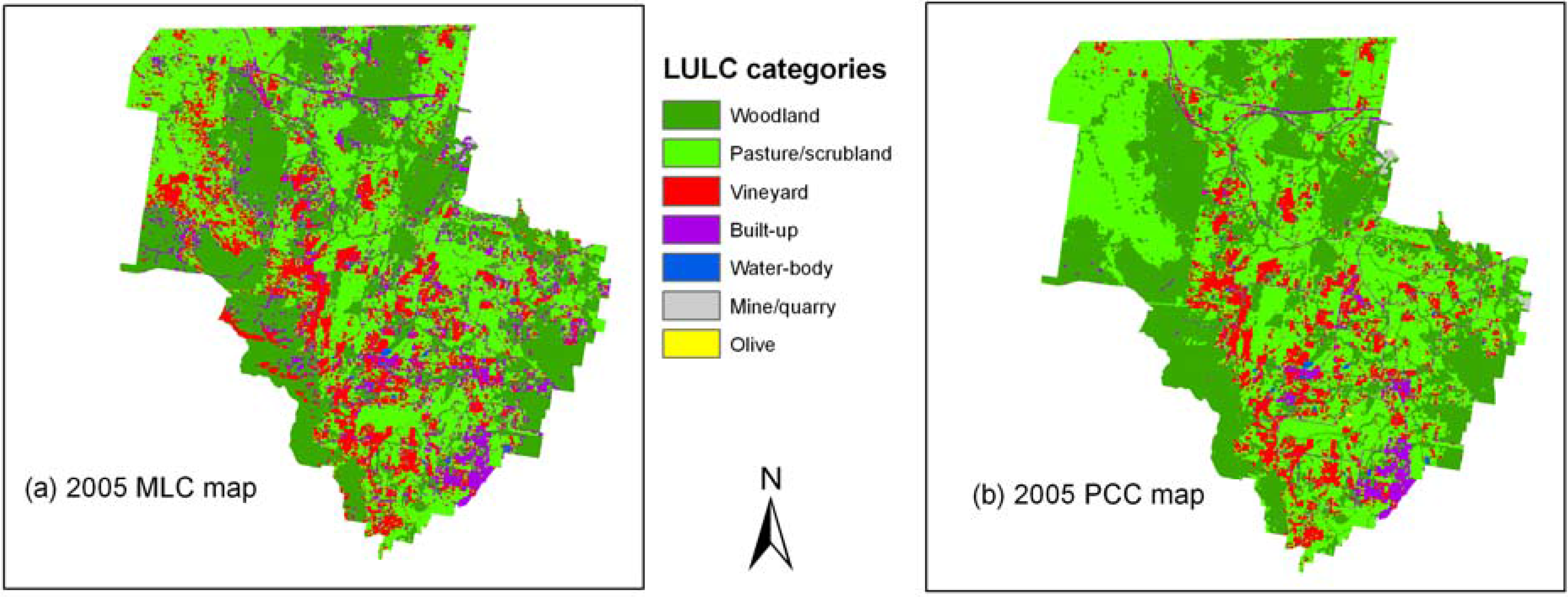
Upon post-classification correction that involved integrating ancillary information in hypothesis testing framework of Knowledge Engineer, the commission errors of the Built-up and Vineyard categories and omission error of the Pasture/scrubland categories were largely reduced (Table 3). These results were quite encouraging. The identification of Built-up category was improved as indicated by increased user’s accuracy from less than 60% to greater than 80% accuracy in all of the three time steps of our analysis. Similarly, the user’s accuracy of Vineyard category increased to above 70%, and producer’s accuracy of Pasture/scrubland improved to above 80%. The overall accuracies of all three PCC maps were above 85%, and Kappa statistics are well above 0.8, indicating a strong agreement or accuracy between the classification map and the ground reference information [26]. It is obvious that the misclassified patches of vineyards in the western forest as well as in the military reserve have disappeared in addition to the reduction of overly estimated Built-up patches resulted from MLC classification (see Figure 3 for example).
Although MLC is one of the most widely used classifiers, it requires input samples to have normal distribution, which makes it to be heavily dependent on statistics. The recent approach is to let the geographical data “have a stronger voice” rather than let statistically derived parameters dictate the analysis [33]. Integration of remotely sensed data with other sources of georeferenced information, such as previous land use data, spatial texture, and digital elevation models (along with their derivatives: slope, aspect, etc.), geology, soils, hydrology, transportation network, vegetation, enable us to achieve greater classification accuracy [9,14,33,34].
Figure 3. Classified maps: (a) MLC and (b) PCC maps for 2005.
Remotesensing 01 00330 g003

4.2. Classifier Performance

Table 4 shows McNemar’s test results with the number of pixels correctly or wrongly classified by MLC and PCC methods. The symbol, f11, denotes the number of cases wrongly classified by both MLC and PCC classifier while f22 denotes the number of cases correctly classified by both the classifiers, while f12 and f21 are the cases that are correctly classified by one classifier but wrongly classified by the other. The table indicates the classifiers agree on f22 and f11 cases but disagree on f12 and f21 cases. The McNemar’s test clearly shows significant improvement of the PCC maps over the MLC maps (Table 4).
Table 4. McNemar’s test showing the superiority of PCC maps vs. MLC maps.
Yearf11f12f21f22Total Chi-square (χ2)P value
1985 maps3479128640076.1<0.001
1995 maps32651130241038.4<0.001
2005 maps4639931641018.8<0.001
f11- number of cases with wrong classification in both maps; classifier 1 (MLC) and classifier 2 ( PCC)
f12- denotes number of cases that are wrongly classified by MLC but correctly classified by PCC
f21- number of cases that are correctly classified by MLC but wrongly classified by PCC and
f22- number of cases with correct classification in both MLC and PCC maps

4.3. Maps and Area Statistics of PCC Classifications
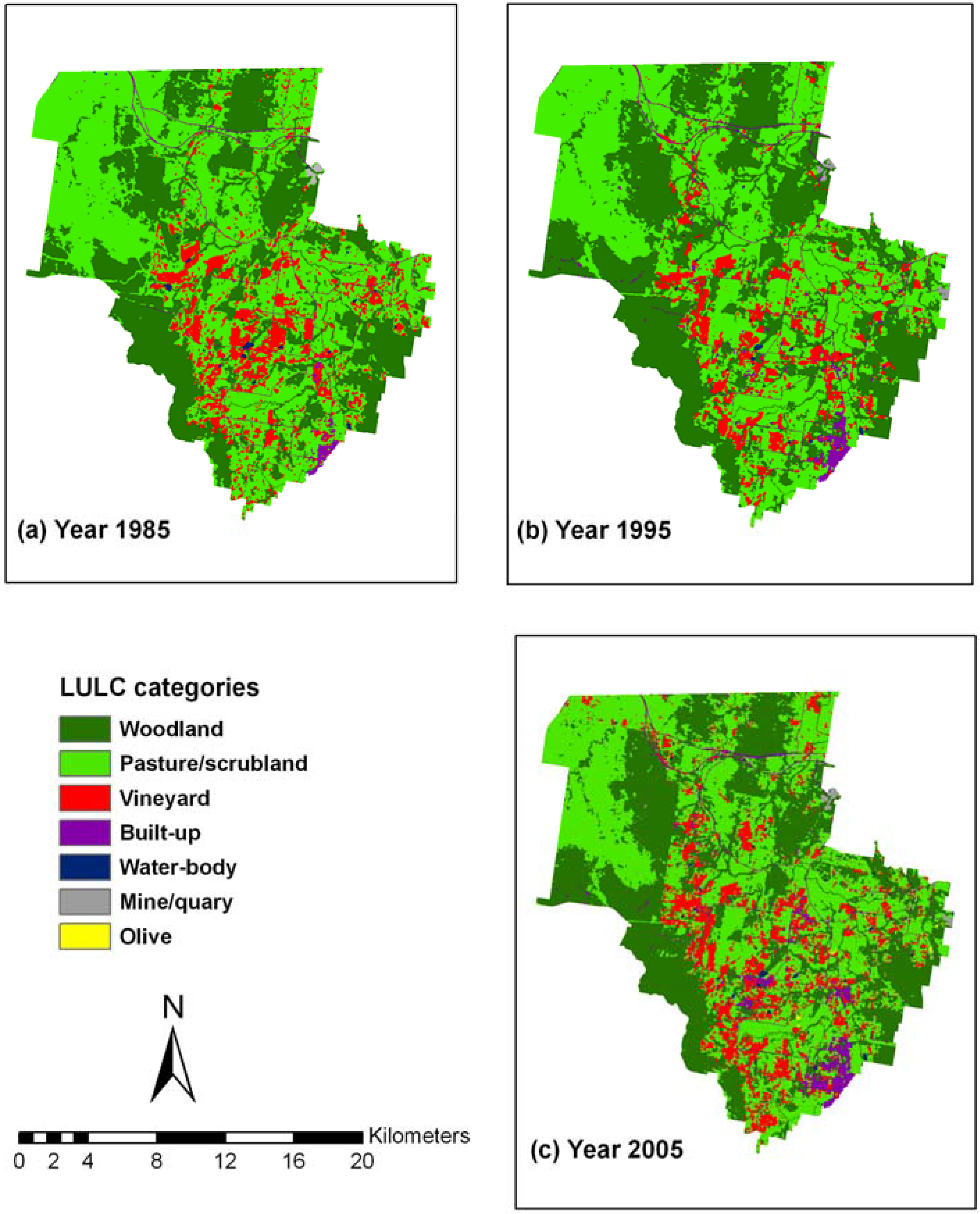
The final maps derived from PCC classification are shown in Figure 4. When each LULC type was compared among the different years, the result indicated that Pasture/scrubland contracted from 53% (of total land of the area) in 1985 to 48.9% in 1995 and then to 46.2% in 2005 (Table 5).
Figure 4. Post classification corrected maps for the years: (a) 1985, (b) 1995 and (c) 2005.
Remotesensing 01 00330 g004
In contrast, Built-up category sequentially increased from 2.0% in 1985 to 2.8% in 1995, and then more than doubled to 4.2% in 2005. However, Vineyards and Woodland categories show inconsistent trends; in the case of Vineyard, it decreased from 9.9% in 1985 to 7.9% in 1995, and then increased by 3% to 10.9% in 2005. On the other hand Woodland area increased from 34.7% in 1985 to 40.1% in 1995, and then decreased to 38% by 2005. In 20 years from 1985 to 2005, all types of LULC were found to have increased except Pasture/scrubland (Table 5). Broadly speaking, more than 95% of the study area is constituted of three LULC categories; Pasture/scrubland, Woodland and Vineyard in all three time steps.
Table 5. Summary of Area statistics based on PCC maps for 1985, 1995 and 2005.
LULC category198519952005Relative change 1985-2005 (%)
Area (ha)% oftotal landArea (ha)% of total landArea (ha)% of total land
Woodland13,156.134.715,190.940.114,412.638.09.6
Pasture/scrubland20,078.853.018,526.648.917,526.946.2-12.7
Vineyard3,766.19.92,983.17.94,147.110.910.1
Built-up757.02.01,050.72.81,580.34.2108.8
Water-body95.30.377.10.2118.20.324.1
Mine/quarry60.70.285.60.282.30.235.6
Olive 46.50.1new LULC
Total37,913.910037,913.910037,913.910012.4

5. Conclusions

Although the MLC is a widely used classifier, it could not perform satisfactorily in deriving accurate and reliable classification of Built-up and Vineyard LULC categories. In this study, we were able to significantly improve MLC maps by incorporating additional data, such as land use, DEM, spatial texture and NDVI value of the Landsat imagery using a hypothesis testing framework based system of classification. The resulting PCC maps can be satisfactorily used for detailed post-classification change detection. This study has demonstrated the usefulness of integrating ancillary data and knowledge-based rules into a classification scheme to improve accuracy of LULC classification.

Acknowledgements

The support of the NSW Department of Natural Resources for providing land use data is greatly acknowledged. We would also like to thank Mr Ken Bray, Mr. Ian Martin and Late Mr Trevor Drayton for their kind help on validating some field information. The first author would also like to thank the Australian Government for providing Endeavour International Postgraduate Research Scholarship to pursue her study in the University of Sydney.

References and Notes

  1. Lambin, E.F.; Turner, B.L.; Geist, H.J.; Agbola, S.B.; Angelsen, A.; Bruce, J.W.; Coomes, O.T.; Dirzo, R.; Fischer, G.; Folke, C.; George, P.S.; Homewood, K.; Imbernon, J.; Leemans, R.; Li, X.; Moran, E.F.; Mortimore, M.; Ramakrishnan, P.S.; Richards, J.F.; Skanes, H.; Steffen, W.; Stone, G.D.; Svedin, U.; Veldkamp, T.A.; Vogel, C.; Xu, J. The causes of land use and land cover change: Moving beyond the myths. Glob. Environ. Change 2001, 11, 261–269. [Google Scholar] [CrossRef]
  2. Goldewijk, K. K.; Ramankutty, N. Land cover change over the last three centuries due to human activities: the availability of new global data sets. Geo. J. 2004, 61, 335–344. [Google Scholar] [CrossRef]
  3. Steele, B.M.; Winne, J.C.; Redmond, R.L. Estimation and mapping of misclassification probabilities for thematic land cover maps. Remote Sens. Environ. 1998, 66, 192–202. [Google Scholar] [CrossRef]
  4. Lu, D.; Weng, Q. A survey of image classification methods and techniques for improving classification performance. Int. J. Remote Sens. 2007, 28, 823–870. [Google Scholar] [CrossRef]
  5. Stow, D.A.; Collins, D.; McKinsey, D. Land use change detection based on multi date imagery from different satellite sensor systems. Geocart. Int. 1990, 5, 3–12. [Google Scholar] [CrossRef]
  6. Foody, G.M. Status of land cover classification accuracy assessment. Remote Sens. Environ. 2002, 80, 185–201. [Google Scholar] [CrossRef]
  7. Wilkinson, G.G. Results of implications of a study of fifteen years of satellite classification experiments. IEEE Trans. Geosci. Remote Sens. 2005, 43, 433–440. [Google Scholar] [CrossRef]
  8. Jensen, J.R. Thematic information extraction: pattern recognition. In Introductory Digital Image Processing – A Remote Sensing Perspective, 3rd ed.; Keith, C.C., Ed.; Prentice Hall Series in Geographic Information Science: Saddle River, NJ, USA, 2005b; pp. 337–406. [Google Scholar]
  9. Stefanov, W.L.; Ramsey, M.S.; Christensen, P.R. Monitoring urban land cover change: An expert system approach to land cover classification of semiarid to arid urban centers. Remote Sens. Environ. 2001, 77, 173–185. [Google Scholar] [CrossRef]
  10. Xiuwan, C. Using remote sensing and GIS to analyse land cover change and its impacts on regional sustainable development. Int. J. Remote Sens. 2002, 23, 107–124. [Google Scholar] [CrossRef]
  11. Currit, N. Development of remotely sensed, historical land cover change database for rural Chihuahua, Mexico. Int. J. Appl. Earth Obs. Geoinf. 2005, 7, 232–247. [Google Scholar] [CrossRef]
  12. Yuan, F.; Sawaya, K.E.; Loeffelholz, B.C.; Bauer, M. E. Land cover classification and change analysis of the Twin Cities (Minnesota) Metropolitan Area by multitemporal Landsat Remote Sensing. Remote Sens. Environ. 2005, 98, 317–328. [Google Scholar] [CrossRef]
  13. Qian, Y.; Zhang, K.; Qiu, F. Spatial contextual noise removal for post classification smoothing of remotely sensed images. ACM Symp. Appl. Comput. 2005, 524–528. [Google Scholar]
  14. Judex, M.; Thamm, M.J.; Menz, G. Improving land cover classification with a knowledge based approach and ancillary data. In Proceeding of the workshop of the EARSeL sig on Land Use and Land Cover 2006, Bonn, Germany, September 28–30, 2006; pp. 184–191.
  15. Yang, X.; Lo, C.P. Using a time series of satellite imagery to detect land use and land cover changes in the Atlanta, Georgia Metropolitan Area. Int. J. Remote Sens. 2002, 23, 1775–1798. [Google Scholar] [CrossRef]
  16. Lower Hunter Regional Strategy; Department of Planning State of New South Wales: Parramatta, New South Wales, Australia, 2006.
  17. Holmes, J.; Hartig, K. Metropolitan colonization and the reinvention of place: class polarization along the Cessnock- Pokolbin Fault Line. Geograph. Res. 2007, 45, 54–70. [Google Scholar] [CrossRef]
  18. Bailly, J.S.; Arnaud, M.; Puech, C. Boosting: a classification method for remote sensing. Int. J. Remote Sens. 2007, 28, 1687–1710. [Google Scholar] [CrossRef]
  19. Liu, X.H.; Skidmore, A.K.; Oosten, H.V. Integration of classification methods for improvement of land cover map accuracy. ISPRS J. Photogramm. Remote Sens. 2002, 56, 257–268. [Google Scholar] [CrossRef]
  20. Weng, Q. Land use change analysis in the Zhujiang Delta of China using satellite remote sensing, GIS and stochastic modeling. J. Environ. Manage. 2002, 64, 273–284. [Google Scholar] [CrossRef] [PubMed]
  21. ERDAS Field guide; Leica Geosystems Geospatial Imaging, LLC: Norcross, Georgia, USA, 2005.
  22. Smits, P.C.; Dellepaine, S.G.; Schowengerdt, R.A. Quality assessment of image classification algorithms for land cover mapping: a review and a proposal for a cost based approach. Int. J. Remote Sens. 1999, 20, 1461–1486. [Google Scholar] [CrossRef]
  23. Plourde, L.; Congalton, R.G. Sampling method and sample placement: How do they affect the accuracy of remotely sensed maps? Photogramm. Eng. Remote Sens. 2003, 69, 289–297. [Google Scholar] [CrossRef]
  24. Anderson, J.R.; Hardy, E.E.; Roach, J.T.; Witmer, R.E. A Land Use and Land Cover Classification System for Use with Remote Sensor Data; Government Printing Office: Washington, DC, USA, 1976.
  25. Congalton, R.G. A review of assessing the accuracy of classification of remotely sensed data. Remote Sens. Environ. 1991, 37, 35–46. [Google Scholar] [CrossRef]
  26. Jensen, J.R. Thematic map accuracy assessment. In Introductory Digital Image Processing–A Remote Sensing Perspective, 3rd ed.; Keith, C.C., Ed.; Prentice Hall Series in Geographic Information Science: Saddle River, NJ, USA, 2005; Sect. C; pp. 495–515. [Google Scholar]
  27. Liu, C.; Frazier, P.; Kumar, L. Comparative assessment of the measures of thematic classification accuracy. Remote Sens. Environ. 2007, 107, 606–616. [Google Scholar] [CrossRef]
  28. Lunetta, R.S.; Congalton, R.G.; Fenstermaker, L.K.; Jensen, J.R.; Tinney, L.R. Remote sensing and geographic information system data integration: error sources and research issues. Photogramm. Eng. Remote Sens. 1991, 57, 677–687. [Google Scholar]
  29. Foody, G.M. Thematic map comparison: evaluating the statistical significance of differences in classification accuracy. Photogramm. Eng. Remote Sens. 2004, 70, 627–633. [Google Scholar] [CrossRef]
  30. De Leeuw, J.; Jia, H.; Yang, L.; Liu, X.; Schmidt, K.; Skidmore, A.K. Comparing accuracy assessments to infer superiority of image classification methods. Int. J. Remote Sens. 2006, 27, 223–232. [Google Scholar] [CrossRef]
  31. Foody, G.M. Map comparison in GIS. Progr.Phys. Geog. 2007, 31, 439–445. [Google Scholar] [CrossRef]
  32. Lu, D.; Moran, E.; Batistella, M. Linear mixture model applied to Amazonian vegetation classification. Remote Sens. Environ. 2003, 87, 456–469. [Google Scholar] [CrossRef] [Green Version]
  33. Jensen, J.R. Information extraction using artificial intelligence. In Introductory Digital Image Processing – A Remote Sensing Perspective, 3rd ed.; Keith, C.C., Ed.; Prentice Hall Series in Geographic Information Science: Saddle River, NJ, USA, 2005; Sect. D; pp. 407–429. [Google Scholar]
  34. Stuckens, J.; Coppin, P.R.; Bauer, M.E. Integrating contextual information with per-pixel classification for improved land cover classification. Remote Sens. Environ. 2000, 71, 282–296. [Google Scholar] [CrossRef]