
Nonprofits and C Corporations: Performance Comparison


Abstract
:1. Introduction
2. Background and Literature Review
2.1. Key Features of Nonprofits (NPs) and C Corporations (CCs)
2.2. Equity and Debt Financing for Nonprofits (NPs) and C Corporations (CCs)
2.3. Assignment of Unlevered and Levered Tax Rates for Nonprofits (NPs) and C Corporations (CCs)
2.3.1. Low “L” Tax Rate Tests
2.3.2. High “H” Tax Rate Tests
2.4. Capital Structure Theory
3. Methodology
We also briefly overview prior research that details how the CSM is used to identify optimal outcomes such as maximum firm value (max VL) and the optimal credit rating (OCR). We then present the method to get costs of borrowing using credit spreads that are matched to interest coverage ratios. This procedure holds a key to discovering max VL and OCR.
3.1. Capital Structure Model (CSM)
3.2. Identifying the Optimal P Choice for Growth and Nongrowth Situations
3.3. P Choices, Costs of Borrowing, and Betas
3.4. Credit Spreads over Time
4. Results Using High (H) Tax Rates under TCJA with Historical Growth
4.1. Variables and Computations
4.2. Illustrations of Large NP and Large CC Outcomes
4.3. Five Illustrative Figures Using TCJA Tax Rates and Growth of 3.12%
5. Results Incorporating Low Tax Rates, TCJA, RTS, and Increased Growth
5.1. ITS Results

| P | PBRBT | gU | EU | Max VL | Max GL | Max %∆EU | NB | ODV | OCR | DGN | |
|---|---|---|---|---|---|---|---|---|---|---|---|
| Panel A. Nongrowth: Pre-TCJA | |||||||||||
| NP-L | 0.3663 | 0.0000 | 0.00% | 11.993 | 12.368 | 0.375 | 3.13% | 8.53% | 0.3552 | A3 | n.a. |
| NP-H | 0.3890 | 0.0000 | 0.00% | 10.710 | 11.548 | 0.838 | 7.82% | 20.11% | 0.3608 | A3 | n.a. |
| CC-L | 0.4500 | 0.0000 | 0.00% | 7.472 | 8.600 | 1.128 | 15.10% | 33.56% | 0.3909 | Baa2 | n.a. |
| CC-H | 0.4594 | 0.0000 | 0.00% | 6.509 | 7.786 | 1.277 | 19.62% | 42.69% | 0.3841 | Baa2 | n.a. |
| Ave | 0.4162 | 0.0000 | 0.00% | 9.171 | 10.075 | 0.904 | 11.42% | 26.22% | 0.3727 | Baa2/A3 | n.a. |
| Panel B. Nongrowth: TCJA | |||||||||||
| NP-L | 0.3663 | 0.0000 | 0.00% | 11.993 | 12.368 | 0.375 | 3.13% | 8.53% | 0.3552 | A3 | n.a. |
| NP-H | 0.3838 | 0.0000 | 0.00% | 11.053 | 11.776 | 0.723 | 6.54% | 17.04% | 0.3602 | A3 | n.a. |
| CC-L | 0.3562 | 0.0000 | 0.00% | 8.646 | 9.498 | 0.853 | 9.86% | 27.68% | 0.3242 | A3 | n.a. |
| CC-H | 0.3601 | 0.0000 | 0.00% | 7.911 | 8.845 | 0.934 | 11.81% | 32.78% | 0.3221 | A3 | n.a. |
| Ave | 0.3666 | 0.0000 | 0.00% | 9.901 | 10.622 | 0.721 | 7.83% | 21.51% | 0.3404 | A3 | n.a. |
| Panel C. 3.12% Growth: Pre-TCJA | |||||||||||
| NP-L | 0.3451 | 0.1938 | 2.00% | 12.729 | 13.292 | 0.563 | 4.42% | 12.82% | 0.3305 | A3 | 0.924 |
| NP-H | 0.3682 | 0.2144 | 2.14% | 11.317 | 12.146 | 0.829 | 7.33% | 19.90% | 0.3430 | A3 | 0.598 |
| CC-L | 0.4569 | 0.2692 | 2.15% | 7.358 | 8.284 | 0.926 | 12.59% | 27.56% | 0.4058 | Baa2 | −0.316 |
| CC-H | 0.4747 | 0.2933 | 2.25% | 6.300 | 7.319 | 1.020 | 16.19% | 34.10% | 0.4086 | Baa2 | −0.467 |
| Ave | 0.4112 | 0.2427 | 2.14% | 9.426 | 10.260 | 0.835 | 10.13% | 23.59% | 0.3720 | Baa2/A3 | 0.185 |
| Panel D. 3.12% Growth: TCJA | |||||||||||
| NP-L | 0.3451 | 0.1938 | 2.00% | 12.729 | 13.292 | 0.563 | 4.42% | 12.82% | 0.3305 | A3 | 0.924 |
| NP-H | 0.3624 | 0.2078 | 2.10% | 11.703 | 12.469 | 0.766 | 6.54% | 18.05% | 0.3402 | A3 | 0.693 |
| CC-L | 0.3462 | 0.2522 | 2.28% | 8.895 | 9.653 | 0.757 | 8.51% | 24.58% | 0.3190 | A3 | 0.154 |
| CC-H | 0.3514 | 0.2607 | 2.32% | 8.107 | 8.908 | 0.800 | 9.87% | 28.09% | 0.3199 | A3 | 0.062 |
| Ave | 0.3513 | 0.2286 | 2.18% | 10.359 | 11.080 | 0.722 | 7.34% | 20.89% | 0.3274 | A3 | 0.458 |
| Panel E. 3.90% Growth: TCJA | |||||||||||
| NP-L | 0.3337 | 0.2297 | 2.49% | 13.164 | 13.940 | 0.776 | 5.90% | 17.67% | 0.3151 | A3 | 1.572 |
| NP-H | 0.3501 | 0.2446 | 2.59% | 12.116 | 13.046 | 0.930 | 7.68% | 21.93% | 0.3251 | A3 | 1.270 |
| CC-L | 0.3346 | 0.2931 | 2.80% | 9.202 | 10.043 | 0.840 | 9.13% | 27.29% | 0.3066 | A3 | 0.544 |
| CC-H | 0.3396 | 0.3021 | 2.85% | 8.391 | 9.258 | 0.867 | 10.33% | 30.43% | 0.3078 | A3 | 0.412 |
| Ave | 0.3395 | 0.2674 | 2.68% | 10.718 | 11.572 | 0.853 | 8.26% | 24.33% | 0.3137 | A3 | 0.950 |
| Panel F. 4.50% Growth: TCJA | |||||||||||
| NP-L | 0.3231 | 0.2556 | 2.86% | 13.596 | 14.625 | 1.029 | 7.57% | 23.42% | 0.3004 | A3 | 2.257 |
| NP-H | 0.3386 | 0.2709 | 2.97% | 12.527 | 13.665 | 1.138 | 9.08% | 26.82% | 0.3104 | A3 | 1.889 |
| CC-L | 0.3234 | 0.3217 | 3.20% | 9.523 | 10.483 | 0.960 | 10.09% | 31.19% | 0.2937 | A3 | 0.985 |
| CC-H | 0.3280 | 0.3308 | 3.26% | 8.686 | 9.657 | 0.970 | 11.17% | 34.05% | 0.2951 | A3 | 0.811 |
| Ave | 0.3283 | 0.2948 | 3.07% | 11.083 | 12.107 | 1.024 | 9.48% | 28.87% | 0.2999 | A3 | 1.486 |
5.2. RTS Results
| P | PBRBT | gU | EU | Max VL | Max GL | Max %∆EU | NB | ODV | OCR | DGN | |
|---|---|---|---|---|---|---|---|---|---|---|---|
| Panel A. Nongrowth: Pre-TCJA | |||||||||||
| NP-L | 0.3663 | 0.0000 | 0.00% | 11.993 | 12.368 | 0.375 | 3.12% | 8.53% | 0.3552 | A3 | n.a. |
| NP-H | 0.3890 | 0.0000 | 0.00% | 10.710 | 11.406 | 0.696 | 6.50% | 16.70% | 0.3653 | A3 | n.a. |
| CC-L | 0.3606 | 0.0000 | 0.00% | 7.472 | 8.055 | 0.583 | 7.81% | 21.66% | 0.3344 | A3 | n.a. |
| CC-H | 0.3680 | 0.0000 | 0.00% | 6.509 | 7.183 | 0.674 | 10.36% | 28.14% | 0.3335 | A3 | n.a. |
| Ave | 0.3710 | 0.0000 | 0.00% | 9.171 | 9.753 | 0.582 | 6.95% | 18.76% | 0.3471 | A3 | n.a. |
| Panel B. Nongrowth: TCJA | |||||||||||
| NP-L | 0.3663 | 0.0000 | 0.00% | 11.993 | 12.368 | 0.375 | 3.12% | 8.53% | 0.3552 | A3 | n.a. |
| NP-H | 0.3838 | 0.0000 | 0.00% | 11.053 | 11.678 | 0.625 | 5.66% | 14.74% | 0.3632 | A3 | n.a. |
| CC-L | 0.3562 | 0.0000 | 0.00% | 8.646 | 9.123 | 0.477 | 5.52% | 15.49% | 0.3375 | A3 | n.a. |
| CC-H | 0.3601 | 0.0000 | 0.00% | 7.911 | 8.460 | 0.549 | 6.93% | 19.25% | 0.3368 | A3 | n.a. |
| Ave | 0.3666 | 0.0000 | 0.00% | 9.901 | 10.407 | 0.506 | 5.31% | 14.50% | 0.3482 | A3 | n.a. |
| Panel C. 3.12% Growth: Pre-TCJA | |||||||||||
| NP-L | 0.3451 | 0.1938 | 2.00% | 12.729 | 13.292 | 0.563 | 4.42% | 12.82% | 0.3305 | A3 | 0.924 |
| NP-H | 0.3653 | 0.1981 | 2.06% | 11.406 | 12.177 | 0.771 | 6.76% | 18.51% | 0.3421 | A3 | 0.771 |
| CC-L | 0.3381 | 0.1997 | 2.08% | 8.362 | 9.034 | 0.673 | 8.04% | 23.79% | 0.3129 | A3 | 0.979 |
| CC-H | 0.3443 | 0.2027 | 2.12% | 7.303 | 8.026 | 0.723 | 9.90% | 28.77% | 0.3132 | A3 | 0.843 |
| Ave | 0.3482 | 0.1986 | 2.07% | 9.950 | 10.632 | 0.683 | 7.28% | 20.97% | 0.3247 | A3 | 0.879 |
| Panel D. 3.12% Growth: TCJA | |||||||||||
| NP-L | 0.3451 | 0.1938 | 2.00% | 12.729 | 13.292 | 0.563 | 4.42% | 12.82% | 0.3305 | A3 | 0.924 |
| NP-H | 0.3606 | 0.1971 | 2.05% | 11.762 | 12.489 | 0.727 | 6.18% | 17.13% | 0.3397 | A3 | 0.810 |
| CC-L | 0.3348 | 0.1969 | 2.04% | 9.199 | 9.782 | 0.583 | 6.34% | 18.95% | 0.3148 | A3 | 0.660 |
| CC-H | 0.3380 | 0.1987 | 2.07% | 8.430 | 9.052 | 0.622 | 7.38% | 21.85% | 0.3148 | A3 | 0.592 |
| Ave | 0.3446 | 0.1966 | 2.04% | 10.530 | 11.154 | 0.624 | 6.08% | 17.69% | 0.3249 | A3 | 0.747 |
| Panel E. 3.90% Growth: TCJA | |||||||||||
| NP-L | 0.3337 | 0.2297 | 2.49% | 13.164 | 13.940 | 0.776 | 5.90% | 17.67% | 0.3151 | A3 | 1.572 |
| NP-H | 0.3484 | 0.2328 | 2.53% | 12.174 | 13.086 | 0.912 | 7.50% | 21.51% | 0.3241 | A3 | 1.408 |
| CC-L | 0.3234 | 0.2328 | 2.53% | 9.523 | 10.266 | 0.743 | 7.80% | 24.13% | 0.3000 | A3 | 1.143 |
| CC-H | 0.3263 | 0.2346 | 2.56% | 8.732 | 9.499 | 0.768 | 8.79% | 26.94% | 0.2999 | A3 | 1.039 |
| Ave | 0.3330 | 0.2325 | 2.53% | 10.898 | 11.698 | 0.800 | 7.50% | 22.56% | 0.3098 | A3 | 1.291 |
| Panel F. 4.50% Growth: TCJA | |||||||||||
| NP-L | 0.3231 | 0.2556 | 2.86% | 13.596 | 14.625 | 1.029 | 7.57% | 23.42% | 0.3004 | A3 | 2.257 |
| NP-H | 0.3371 | 0.2585 | 2.91% | 12.582 | 13.722 | 1.140 | 9.06% | 26.87% | 0.3091 | A3 | 2.043 |
| CC-L | 0.3128 | 0.2587 | 2.91% | 9.845 | 10.781 | 0.936 | 9.50% | 30.38% | 0.2856 | A3 | 1.658 |
| CC-H | 0.3155 | 0.2603 | 2.93% | 9.030 | 9.973 | 0.944 | 10.45% | 33.13% | 0.2857 | A3 | 1.513 |
| Ave | 0.3221 | 0.2583 | 2.90% | 11.263 | 12.275 | 1.012 | 9.14% | 28.45% | 0.295 | A3 | 1.868 |
5.3. Limitations and Future Research
6. Discussion
7. Materials and Methods
8. Conclusions
Funding
Informed Consent Statement
Data Availability Statement
Acknowledgments
Conflicts of Interest
References
- Anheier, Helmut. 2014. Nonprofit Organizations. Theory, Management, Policy, 2nd ed. New York: Routledge, pp. 1–594. [Google Scholar]
- Baxter, Nevins. 1967. Leverage risk of ruin and the cost of capital. Journal of Finance 22: 395–403. [Google Scholar]
- Berk, Jonathan, Richard Stanton, and Josef Zechner. 2010. Human capital, bankruptcy and capital structure. Journal of Finance 65: 891–926. [Google Scholar] [CrossRef] [Green Version]
- Bowman, Woods. 2002. The uniqueness of NP finance and the decision to borrow. NP Management and Leadership 23: 293–311. [Google Scholar]
- Bowman, Woods. 2015. The Price of NPO Debt. NP Quarterly. Available online: https://NPquarterly.org/2015/08/06/the-price-of-NP-debt/ (accessed on 31 December 2019).
- Brookings. 2017. 9 Facts about Pass-through Businesses. Available online: https://www.brookings.edu/research/9-facts-about-pass-through-businesses/#fact5 (accessed on 19 December 2019).
- Calabrese, Thad. 2011. Testing competing capital structure theories of nonprofit organizations. Public Budgeting and Finance 31: 119–43. [Google Scholar] [CrossRef]
- Calabrese, Thad, and Todd Ely. 2016. Borrowing for the public good: The growing importance of tax-exempt bonds for public charities. Nonprofit and Voluntary Sector Quarterly 45: 458–77. [Google Scholar] [CrossRef]
- Damodaran, Aswath. 2021. Damodaran Online: Home Page for Aswath Damodaran. Available online: http://pages.stern.nyu.edu/~adamodar/New_Home_Page/datacurrent.html (accessed on 15 January 2021).
- DeAngelo, Harry, and Ronald Masulis. 1980. Optimal capital structure under corporate and personal taxes. Journal of Financial Economics 8: 3–29. [Google Scholar] [CrossRef]
- Donaldson, Gordon. 1961. Corporate Debt Capacity: A Study of Corporate Debt Policy and the Determination of Corporate Debt Capacity. Boston: Harvard Business School, pp. 1–294. [Google Scholar]
- Farrar, Donald, and Lee Selwyn. 1967. Taxes, corporate policy, and return to investors. National Tax Journal 20: 444–54. [Google Scholar] [CrossRef]
- Federal Reserve Economic Data. 2020. 30-Year Treasury Constant Maturity Rate. Federal Reserve Bank of St. Louis. Available online: https://fred.stlouisfed.org/series/DGS30 (accessed on 25 July 2020).
- Graham, John. 2000. How big are the tax benefits of debt? Journal of Finance 55: 1901–41. [Google Scholar] [CrossRef]
- Graham, John, and Campbell Harvey. 2001. The theory and practice of corporate finance: Evidence from the field. Journal of Financial Economics 60: 187–243. [Google Scholar] [CrossRef]
- Hackbarth, Dirk, Christopher Hennessy, and Hayne Leland. 2007. Can the trade-off theory explain debt structure? Review of Financial Studies 20: 1389–428. [Google Scholar] [CrossRef] [Green Version]
- Hull, Robert. 2005. Firm value and the debt-equity choice. Regional Business Review 24: 50–75. [Google Scholar]
- Hull, Robert. 2010. A capital structure model with growth. Investment Management and Financial Innovation 7: 26–40. [Google Scholar]
- Hull, Robert. 2012. A capital structure model with wealth transfers. Investment Management and Financial Innovation 9: 19–32. [Google Scholar]
- Hull, Robert. 2014. A capital structure model (CSM) with tax rate changes. Investment Management and Financial Innovations 11: 8–21. [Google Scholar]
- Hull, Robert. 2018. Capital structure model (CSM): Correction, constraints, and applications. Investment Management and Financial Innovation 15: 245–62. [Google Scholar] [CrossRef] [Green Version]
- Hull, Robert. 2019. Business wealth and tax policy. Theoretical Economics Letters 9: 1020–39. [Google Scholar] [CrossRef] [Green Version]
- Hull, Robert. 2020a. Credit ratings and firm value. Investment Management and Financial Innovation 17: 157–68. [Google Scholar] [CrossRef]
- Hull, Robert. 2020b. Pass-through and C corp outputs under TCJA. International Journal of Financial Studies 18: 46. [Google Scholar] [CrossRef]
- Hull, Robert, and David Price. 2015. Pass-through valuation. The Journal of Entrepreneurial Finance 17: 82–116. [Google Scholar] [CrossRef]
- Hull, Robert, and John Hull. 2021. Taxpayer wealth and federal tax revenue under a tax policy that shields retained earnings used for growth from taxes. eJournal of Tax Research 19: 48–96. [Google Scholar]
- Hull, Robert, and Shane Van Dalsem. 2021. Nonprofits and pass-throughs: Performance comparison. International Journal of Financial Studies 9: 13. [Google Scholar] [CrossRef]
- Jegers, Marc, and Else Verschueren. 2006. On the capital structure of nonprofit organisations: An empirical study for Californian organisations. Financial Accountability & Management 22: 309–29. [Google Scholar]
- Jensen, Michael. 1986. Agency costs of free cash flow, corporate finance, and takeovers. American Economic Review 76: 323–29. [Google Scholar]
- Jensen, Michael, and William Meckling. 1976. Theory of the firm: Managerial behavior, agency costs and ownership structure. Journal of Financial Economics 3: 305–60. [Google Scholar] [CrossRef]
- Kisgen, Darren. 2006. Credit ratings and capital structure. Journal of Finance 61: 1035–72. [Google Scholar] [CrossRef]
- Korteweg, Arthur. 2010. The net benefits of leverage. Journal of Finance 65: 2137–70. [Google Scholar] [CrossRef]
- Manne, Geoffrey. 1999. Agency costs and the oversight of charitable organizations. Wisconsin Law Review 227: 227–90. [Google Scholar]
- McBride, William. 2012. CRS, at Odds with Academic Studies, Continues to Claim No Harm in Raising Top Earners Tax Rates. Tax Foundation. Available online: https://taxfoundation.org/crs-odds-academic-studies-continues-claim-no-harm-raising-top-earners-tax-rates (accessed on 1 February 2020).
- Miller, Clara. 2003. Hidden in plain sight: Nonprofit capital structure. Nonprofit Quarterly, March 21, 1–8. [Google Scholar]
- Miller, Merton. 1977. Debt and taxes. Journal of Finance 32: 261–75. [Google Scholar]
- Morningstar. 2019. Credit Ratings. Available online: https://ratingagency.morningstar.com/mcr/ratings-surveillance/corporate-financial%20institutions (accessed on 24 August 2021).
- Myers, Stewart. 1977. Determinants of corporate borrowing. Journal of Financial Economics 5: 147–75. [Google Scholar] [CrossRef] [Green Version]
- Myers, Stewart, and Nicholas Majluf. 1984. Corporate financing and investment decisions when firms have information that investors do not have. Journal of Financial Economics 13: 187–221. [Google Scholar] [CrossRef] [Green Version]
- National Center for Charitable Statistics. 2018. The Nonprofit Sector in Brief 2018. Available online: https://nccs.urban.org/publication/nonprofit-sector-brief-2018#the-nonprofit-sector-in-brief-2018-public-charites-giving-and-volunteering (accessed on 2 February 2020).
- Tax Foundation. 2018. The Tax Foundation’s Tax and Growth Model, April. Available online: https://taxfoundation.org/overview-tax-foundations-taxes-growth-model/ (accessed on 20 May 2020).
- Tax Policy Center. 2020. How Do Taxes Affect the Economy in the Long Run? Available online: https://www.taxpolicycenter.org/briefing-book/how-do-taxes-affect-economy-long-run (accessed on 20 May 2020).
- Trussell, John. 2012. A comparison of the capital structures of nonprofit and proprietary healthcare organizations. Journal of Healthcare and Finance 39: 1–12. [Google Scholar]
- US Bureau of Economic Analysis. 2020. US Real GDP Growth Rate by Year. Available online: http://www.multpl.com/us-real-gdp-growth-rate/table/by-year (accessed on 11 January 2020).
- Van Binsbergen, Jules, John Graham, and Jie Yang. 2010. Cost of debt. Journal of Finance 65: 2089–36. [Google Scholar] [CrossRef]


| Nonprofit | C Corp |
|---|---|
| Owned By: No individuals | Owned By: Individual investors |
| Ownership categories: Corporation (501c3), association, trust | Ownership categories: C corp (files its own tax return using Form 1120) |
| Board Members: Nominated | Board Members: Elected by equity owners |
| Official obligations: Fulfill duties related to goals involving service, education, and research | Official obligations: Increase ownership wealth by providing profitable services and products |
| Major Goal: Maximize value in terms of service distributions | Major Goal: Maximize value in terms of monetary distributions |
| Mission: Described largely in terms of service, education, research, and growth | Mission: Described largely in terms of profit, efficiency, service, and growth |
| Decision-making and implementation: Cautiously proceeds to satisfy mission and constituencies | Decision-making and implementation: Quickly responds to profitable opportunities |
| Sources of Revenues: Services, contributions, grants, and investments (including endowment income) | Sources of Revenues: Business activities (sales and services) and investments in other businesses |
| Equity Distributions: Non-monetary distributions in form of services rendered to those in need | Equity Distributions: Monetary distributions to owners in form of cash payouts and capital gains |
| Sources of Equity Financing: Internal equity (eligible revenues, investment/endowment income); External equity (contributions, grants, government) | Sources of Equity Financing: Internal equity (retained earnings); External equity (new seasoned equity offerings or equity-like offerings such as warrants) |
| Sources of Debt Financing: Personal tax-exempt debt, nonfinancial debt (mortgages), short-term debt (trade credit, bank borrowings avoided as interest not exempt from taxes) | Sources of Debt Financing: Bond issues (various types such as senior, subordinate, callable, convertible, etc.), short-term debt (trade credit, bank borrowings) |
| Corporate Taxes: Only apply to profitable ventures | Corporate Taxes: Apply to taxable corporate earnings |
| Personal Equity Taxes: Zero unless there are taxable for-profit ventures that have distributions | Personal Equity Taxes: Personal taxes paid on dividends and capital gains |
| Personal Debt Taxes: Zero or minor due to issuing mostly tax-exempt debt | Personal Debt Taxes: Personal taxes paid on interest from debt |
| Interest or Retained Earnings Tax Shield: Zero or small tax shields for side ventures that are for-profit | Interest or Retained Earnings Tax Shield: Full business tax shields |
| Nonprofit (unlevered, levered, and target tax rates) | C Corporation (unlevered, levered, and target tax rates) |
| Panel A: Low (L) Tax Rates | |
| Pre-TCJA (target levered rate in parenthesis) | |
| Nonprofit (NP): Tax rates are the same for ITS and RTS | C Corp (CC): Levered tax rates differ for ITS and RTS |
| ITS | |
| TC1 = 0 and TC2 = 0 (0) | TC1 = 0.30 and TC2 = 0.2499 (0.254) |
| TE1 = 0 and TE2 = 0 (0) | TE1 = 0.11 and TE2 = 0. 0916 (0.094) |
| TD1 = 0 and TD2 = 0 (0) | TD1 = 0.15 and TD2 = 0.1791 (0.175) |
| RTS | |
| TC1 = 0.30 and TC2 = 0.2577 (0.254) | |
| TE1 = 0.11 and TE2 = 0. 0945 (0.094) | |
| TD1 = 0.15 and TD2 = 0.1739 (0.175) | |
| TCJA (target levered rate in parenthesis) | |
| Nonprofit (NP): Tax rates are the same for ITS and RTS | C Corp (CC): Tax rates are the same for ITS and RTS |
| TC1 = 0 and TC2 = 0 (0) | TC1 = 0.19 and TC2 = 0.1632 (0.165) |
| TE1 = 0 and TE2 = 0 (0) | TE1 = 0.11 and TE2 = 0. 0945 (0.094) |
| TD1 = 0 and TD2 = 0 (0) | TD1 = 0.14 and TD2 = 0.1623 (0.16) |
| Panel B: High (H) Tax Rates | |
| Pre-TCJA (target levered rate in parenthesis) | |
| Nonprofit (NP): Tax rates are the same for ITS and RTS | C Corp (CC): Levered tax rates differ for ITS and RTS |
| ITS | |
| TC1 = 0.06 and TC2 = 0.0515 (0.05) | TC1 = 0.35 and TC2 = 0.2915 (0.295) |
| TE1 = 0.05 and TE2 = 0.0429 (0.045) | TE1 = 0.165 and TE2 = 0.1374 (0.14) |
| TD1 = 0.0 and TD2 = 0 (0) | TD1 = 0.19 and TD2 = 0.2269 (0.224) |
| RTS | |
| TC1 = 0.35 and TC2 = 0.3006 (0.295) | |
| TE1 = 0.165 and TE2 = 0.1417 (0.14) | |
| TD1 = 0.19 and TD2 = 0.2203 (0.224) | |
| TCJA (target levered rate in parenthesis) | |
| Nonprofit (NP): Tax rates are the same for ITS and RTS | C Corp (CC): Tax rates are the same for ITS and RTS |
| TC1 = 0.04 and TC2 = 0.0343 (0.035) | TC1 = 0.21 and TC2 = 0.1803 (0.18) |
| TE1 = 0.04 and TE2 = 0.0343 (0.035) | TE1 = 0.165 and TE2 = 0.1417 (0.14) |
| TD1 = 0 and TD2 = 0 (0) | TD1 = 0.180 and TD2 = 0.2087 (0.21) |
| P Choice | T C2 | ICR | Moody’s Rating | Credit Spread | rD | rL | βD | βL |
|---|---|---|---|---|---|---|---|---|
| 0.09222051 | 0.0582 | 16.000 | Aaa | 0.69% | 5.64% | 8.44% | 0.1426 | 0.7211 |
| 0.19166453 | 0.0565 | 7.500 | Aa2 | 0.85% | 5.80% | 8.60% | 0.1756 | 0.7541 |
| 0.23123954 | 0.0548 | 6.000 | A1 | 1.07% | 6.02% | 8.82% | 0.2211 | 0.7996 |
| 0.27998121 | 0.0531 | 4.875 | A2 | 1.18% | 6.13% | 8.93% | 0.2438 | 0.8223 |
| 0.36815152 | 0.0515 | 3.625 | A3 | 1.33% | 6.28% | 9.08% | 0.2748 | 0.8533 |
| 0.45834713 | 0.0500 | 2.750 | Baa2 | 1.71% | 6.66% | 9.46% | 0.3533 | 0.9318 |
| 0.48762513 | 0.0485 | 2.375 | Ba1 | 2.31% | 7.26% | 10.06% | 0.4773 | 1.0558 |
| 0.51330250 | 0.0470 | 2.125 | Ba2 | 2.77% | 7.72% | 10.52% | 0.5723 | 1.1508 |
| 0.49974477 | 0.0456 | 1.875 | B1 | 4.05% | 9.00% | 11.80% | 0.8368 | 1.4153 |
| 0.52977557 | 0.0442 | 1.625 | B2 | 4.86% | 9.81% | 12.61% | 1.0041 | 1.5826 |
| 0.56478929 | 0.0429 | 1.375 | B3 | 5.94% | 10.89% | 13.69% | 1.2273 | 1.8058 |
| 0.57334105 | 0.0416 | 1.025 | Caa | 9.46% | 14.41% | 17.21% | 1.9545 | 2.5331 |
| 0.78389816 | 0.0404 | 0.725 | Ca2 | 9.97% | 14.92% | 17.72% | 2.0599 | 2.6384 |
| 1.10736026 | 0.0392 | 0.425 | C2 | 13.09% | 18.04% | 20.84% | 2.7045 | 3.2831 |
| 1.89828374 | 0.0380 | 0.200 | D2 | 17.44% | 22.39% | 25.19% | 3.6033 | 4.1818 |
| Credit Ratings Moody’s/S&P | Credit Spread Statistics by Years/Period (Means for the Eight Years in the Last Column) | ||||||||
|---|---|---|---|---|---|---|---|---|---|
| 2013 | 2014 | 2015 | 2016 | 2017 | 2018 | 2019 | 2020 | 2013–2020 | |
| Aaa/AAA | 0.4000% | 0.4000% | 0.7500% | 0.6000% | 0.5400% | 0.7500% | 0.6300% | 0.6900% | 0.5950% |
| Aa2/AA | 0.7000% | 0.7000% | 1.0000% | 0.8000% | 0.7200% | 1.0000% | 0.7800% | 0.8500% | 0.8188% |
| A1/A+ | 0.8500% | 0.9000% | 1.1000% | 1.0000% | 0.9000% | 1.2500% | 0.9750% | 1.0700% | 1.0056% |
| A2/A | 1.0000% | 1.0000% | 1.2500% | 1.1000% | 0.9900% | 1.3750% | 1.0764% | 1.1800% | 1.1214% |
| A3/A− | 1.3000% | 1.2000% | 1.7500% | 1.2500% | 1.1250% | 1.5625% | 1.2168% | 1.3300% | 1.3418% |
| Baa2/BBB | 2.0000% | 1.7500% | 2.2500% | 1.6000% | 1.2700% | 2.0000% | 1.5600% | 1.7100% | 1.7675% |
| Ba1/BB+ | 3.0000% | 2.7500% | 3.2500% | 2.5000% | 1.9844% | 3.0000% | 2.0000% | 2.3100% | 2.5993% |
| Ba2/BB | 4.0000% | 3.2500% | 4.2500% | 3.0000% | 2.3813% | 3.6000% | 2.4000% | 2.7700% | 3.2064% |
| B1/B+ | 5.5000% | 4.0000% | 5.5000% | 3.7500% | 2.9766% | 4.5000% | 3.5100% | 4.0500% | 4.2233% |
| B2/B | 6.5000% | 5.0000% | 6.5000% | 4.5000% | 3.5719% | 5.4000% | 4.2120% | 4.8600% | 5.0680% |
| B3/B− | 7.2500% | 6.0000% | 7.5000% | 5.5000% | 4.3656% | 6.6000% | 5.1480% | 5.9400% | 6.0380% |
| Caa/CCC | 8.7500% | 7.0000% | 9.0000% | 6.5000% | 8.6369% | 9.0000% | 8.2000% | 9.4600% | 8.3184% |
| Ca2/CC | 9.5000% | 8.0000% | 12.0000% | 8.0000% | 10.6300% | 11.0769% | 8.6424% | 9.9700% | 9.7274% |
| C2/C | 10.5000% | 10.0000% | 16.0000% | 10.5000% | 13.9519% | 14.5385% | 11.3412% | 13.0900% | 12.4902% |
| D2/D | 12.0000% | 12.0000% | 20.0000% | 14.0000% | 18.6025% | 19.3846% | 15.1164% | 17.4400% | 16.0679% |
| Mean | 4.8833% | 4.2633% | 6.1400% | 4.3067% | 4.8431% | 5.6692% | 4.4539% | 5.1147% | 4.9593% |
| StDev | 3.9775% | 3.6493% | 5.8879% | 3.9770% | 5.5564% | 5.5750% | 4.4309% | 5.1321% | 4.7383% |
| Panel A. Alpha Computations for High (H) Tax Rates Pre-TCJA |
| Large Nonprofit (NP) Alpha Computations: |
| For an unlevered situation for the high (H) tax rate scenario for a pre-TCJA tax rate environment and an ITS tax policy, the unlevered personal equity tax rate (TE1) is 0.05, the unlevered corporate tax rate (TC1) = 0.06, and the unlevered personal debt tax rate (TD1) = 0. The latter only exists hypothetically (since unlevered means no debt) but is assigned a beginning value to achieve an effective levered personal tax rate on debt (TD2) at the optimal P choice. TD1 and TD2 are zero because we assume large NPs have enough clout to avoid issuing taxable debt, which is to say all debt they issue can be exempt from personal taxes. Following prior CSM research originating in Hull (2014) and using a 0.03 change in tax rates between P choices, the levered personal equity tax rate (TE2) is less than TE1 since taxes paid by equity owners decrease by 0.03 with each increasing P choice. Similarly, the levered corporate tax rate (TC2) is less than TC1 since corporate taxes decrease by 0.03 with each increasing P choice. If TD1 was not assumed to be zero, TD2 would be greater than TD1 since TD2 increases by 0.03 with each increasing P choice. For the first debt-for-equity choice using TD1 = 0, we have: TD2 = TD1(1 + ΔTD1)1 = 0(1 − 0.03)1 = 0. Using TE1 = 0.05, we have: TE2 = TE1(1 − ΔTE1)1 = 0.05(1 − 0.03)1 = 0.0485. Using TC1 = 0.06, we have: TC2 = TC2(1 − ΔTC2)1 = 0.06(1 − 0.03)1 = 0.0582. Computing the alphas to ten digits (so later computations can minimize rounding off errors), we have: α1 = (1 − TE2)(1 − TC2)/(1 − TD2) = (1 − 0.0485)(1 − 0.0582)/(1 − 0) = 0.8961227000. α2 = (1 − TE2)(1 − TC2)/(1 − TE1)(1 − TC1) = (1 − 0.0485)(1 − 0.0582)/(1 − 0.05)(1 − 0.06) = 1.0034968645. For the fifth (and optimal) debt-for-equity choice using TD2 = TD1(1 + 0.03)5 = 0(0.8587340257) = 0, TE2 = TE1(1 − 0.03)5 = 0.05(0.8587340257) = 0.0429367013, and TC2 = TC1(1 − 0.03)5 = 0.06(0.8587340257) = 0.0515240415, we have: α1 = (1 − TE2)(1 − TC2)/(1 − TD2) = (1 − 0.0429367013)(1 − 0.0515240415)/(1 − 0) = 0.9077515296. α2 = (1 − TE2)(1 − TC2)/(1 − TE1)(1 − TC1) = (1 − 0.0429367013)(1 − 0.0515240415)/(1 − 0.05)(1 − 0.06) = 1.0165190700. |
| Large C Corporation (CC) Alpha Computations: |
| For an unlevered situation for the high (H) tax rate scenario for a pre-TCJA tax rate environment and an ITS tax policy, the unlevered personal equity tax rate (TE1) is 0.165, the unlevered corporate tax rate (TC1) = 0.35, and the beginning personal tax rate on debt income is TD1 = 0.19. For the first debt-for-equity choice using TD1 = 0.19, we have: TD2 = TD1(1 + ΔTD1)1 = 0.19(1 − 0.03)1 = 0.1957. Using TE1 = 0.165, we have: TE2 = TE1(1 + ΔTE1)1 = 0.165(1 − 0.03)1 = 0.16005. Using TC1 = 0.35, we have: TC2 = TC2(1 − ΔTC2)1 = 0.35(1 − 0.03)1 = 0.3395, we have (to ten digits so later computations can minimize rounding off errors): α1 = (1 − TE2)(1 − TC2)/(1 − TD2) = (1 − 0.16005)(1 − 0.3395)/(1 − 0.1957) = 0.6897761718. α2 = (1 − TE2)(1 − TC2)/(1 − TE1)(1 − TC1) = (1 − 0.16005)(1 − 0.3395)/(1 − 0.165)(1 − 0.35) = 1.0221777522. For the sixth (and optimal) debt-for-equity choice using TD2 = TD1(1 + 0.03)6 = 0.19(0.8329720049) = 0.2268699363, TE2 = TE1(1 − 0.03)6 = 0.165(0.8329720049) = 0.1374403808, and TC2 = TC1(1 − 0.03)6 = 0.35(0.8329720049) = 0.2915402017, we have: α1 = (1 − TE2)(1 − TC2)/(1 − TD2) = (1 − 0.1374403808)(1 − 0.2915402017)/(1 − 0.1582646809) = 0.7904088103. α2 = (1 − TE2)(1 − TC2)/(1 − TE1)(1-TC1) = (1 − 0.1374403808)(1 − 0.2915402017)/(1 − 0.165)(1 − 0.35) = 1.1259121397. |
| Panel B. Unlevered Firm Value (EU) Computations |
| NP example using CC definitions given in Section 3.1: PBRBT = 0.2144; CFBT = USD 1,000,000; RE = PBRBT(CFBT) = 0.2144(USD 1,000,000) = USD 214,400. CRE = TC2(RE) = 0.0515240415(USD 214,400) = USD 11,046.75. %CRE per USD 1,000,000 of CFBT = USD 11,046.75/USD 1,000,000 = 0.01104675 or 1.104675% or about 1.10%. C = (1 − PBRBT)(CFBT) = (1 − 0.2144)(USD 1,000,000) = USD 785,600. GU = rU(1 − TC1)RE/C = 0.08338(1 − 0.06)USD 214,400/USD 785,600 = 0.021390112 or 2.1390112%. rUg = rU − gU = 0.08338 − 0.0213901116 = 0.0619898884. EU = (1 − PBRBT)(1 − TE1)(1 − TC1)CFBT/rUg = (1 − 0.2144)(1 − 0.05)(1 − 0.06)USD 1,000,000/0.0619898884 = USD 11,317,020. |
| CC example using CC definitions given in Section 3.1: PBRBT = 0.2933; CFBT = USD 1,000,000; RE = PBRBT(CFBT) = 0.2933(USD 1,000,000) = USD 293,300. CRE = TC2(RE) = 0.2915402017(USD 293,300) = USD 85,508.74. %CRE per USD 1,000,000 of CFBT = USD 85,508.74/USD 1,000,000 = 0.08550874 or 8.55087% or about 8.55%. C = (1 − PBRBT)(CFBT) = (1 − 0.2933)(USD 1,000,000) = USD 706,700. GU = rU(1 − TE1)RE/C = 0.08338(1 − 0.165)USD 293,300/USD 706,700 = 0.0224932505 or 2.249325046%. rUg = rU − gU = 0.065 − 0.0224932505 = 0.0608867495. EU = (1 − PBRBT)(1 − TE1)CFBT/rUg = (1 − 0.2933)(1 − 0.165)USD 1,000,000/0.0608867495 = USD 6,299,588. |
| Panel A. Key Outcomes for P Choices (Optimal Outcomes in Bold Print) | |||||||||
| P Choice = Proportion of Unlevered Firm Value (EU) Retired by Debt (D) | |||||||||
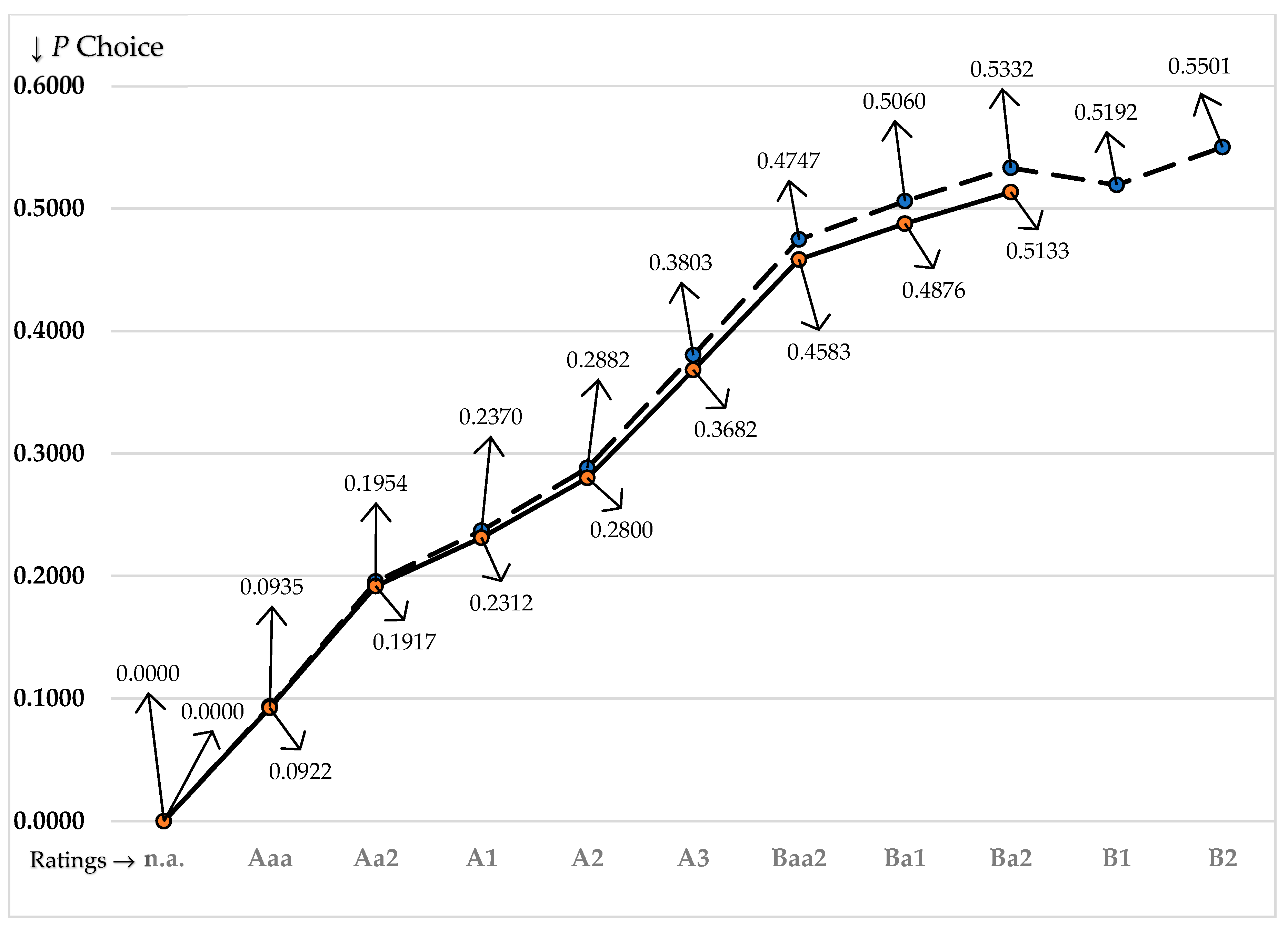
| Outcomes | 0.0000 | 0.0922 | 0.1917 | 0.2312 | 0.2800 | 0.3682 | 0.4583 | 0.4876 | 0.5133 |
| Moody’s Rating | n.a. | Aaa | Aa2 | A1 | A2 | A3 | Baa2 | Ba1 | Ba2 |
| Debt (D) | 0.000 | 1.044 | 2.169 | 2.617 | 3.169 | 4.166 | 5.187 | 5.518 | 5.809 |
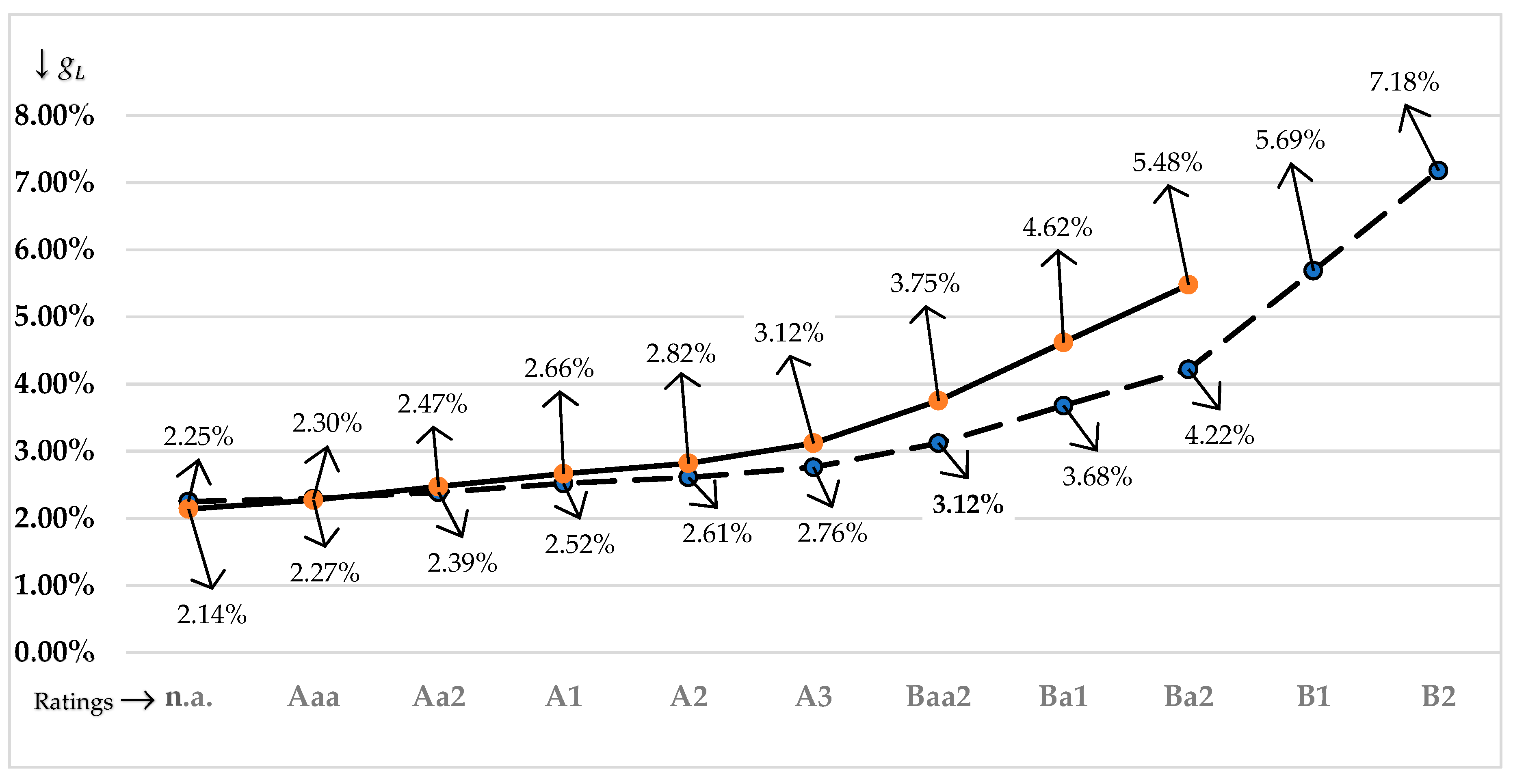
| Equity growth rate: gL | 2.14% | 2.27% | 2.47% | 2.66% | 2.82% | 3.12% | 3.75% | 4.62% | 5.48% |
| Growth adjusted: rLg | 6.20% | 6.17% | 6.13% | 6.16% | 6.11% | 5.96% | 5.71% | 5.44% | 5.04% |
| 1st component of GL | 0.000 | 0.188 | 0.323 | 0.308 | 0.292 | 0.181 | −0.325 | −1.209 | −2.339 |
| 2nd component of GL | 0.000 | 0.098 | 0.213 | 0.195 | 0.319 | 0.648 | 1.217 | 1.874 | 2.956 |
| Gain to leverage: GL | 0.000 | 0.286 | 0.535 | 0.503 | 0.610 | 0.829 | 0.892 | 0.665 | 0.617 |
| Firm value: VL | 11.317 | 11.603 | 11.852 | 11.820 | 11.927 | 12.146 | 12.209 | 11.982 | 11.934 |
| Equity value: EL | 11.317 | 10.560 | 9.683 | 9.203 | 8.759 | 7.980 | 7.022 | 6.464 | 6.125 |
| %∆EU | 0.00% | 2.53% | 4.73% | 4.45% | 5.39% | 7.33% | 7.89% | 5.88% | 5.46% |
| NB | 0.0% | 27.4% | 24.7% | 19.2% | 19.3% | 19.9% | 17.2% | 12.1% | 10.6% |
| DV | 0.0000 | 0.0899 | 0.1830 | 0.2214 | 0.2657 | 0.3430 | 0.4248 | 0.4605 | 0.4868 |
| Panel B. Computations for Optimal Outcomes at P = 0.36815152 | |||||||||
| D = P(EU) = 0.36815152(USD 11,317,020) = USD 4,166,378 or D = −(1 − TD2)I/rD = −(1 − 0)USD 261,648.54/0.0628 = USD 4,166,378. gL = r − (1 − TC2)RE/[C − G − −(1 − TC2)I] = 0.090 − (1 − 0.0515240415)USD 214,400/[USD 785,600 + USD 54,438 − 37 − −(1 − 0.0515240415)USD 261,648.54] = 0.0311967879 or about 3.12%. Thus, rLg = −rL − gL = 0.0–08 − 0.0311967879 = 0.0596032121 or about 5.96%. Max GL = −(1 − αIrD/rLg)D + –(1 − α2rUg/rLg)EU = −[1 − 0.9077515296(0.0628)/0.0596032121]USD 4,166,378 + –[1 − 1.01651907(0.0619898884)/0.0596032121]USD 11,317,020 = USD 181,494 + USD 647,597 = USD 829,091. Max VL = EU + Max GL = USD 11,317,020 + USD 829,091 = USD 12,146,111. EL = −VL − D = USD 12,146,111 − USD 4,166,378 = USD 7,979,733. Max %∆EU = Max GL/EU = USD 829,091/USD 11,317,020 = 0.0733 or 7.33%. NB = Max GL/D = USD 829,091/USD 4,166,378 = 0.1990 or 19.90%. ODV = D/Max VL = USD 4,166,378/USD 12,146,111 = 0.3430. | |||||||||
| Panel A. Key Outcomes for P Choices (Optimal Outcomes in Bold Print) | |||||||||
| P Choice = Proportion of Unlevered Firm Value (EU) Retired by Debt (D) | |||||||||
| Outcomes | 0.0000 | 0.0935 | 0.1954 | 0.2370 | 0.2882 | 0.3803 | 0.4747 | 0.5060 | 0.5332 |
| Moody’s Rating | n.a. | Aaa | Aa2 | A1 | A2 | A3 | Baa2 | Ba1 | Ba2 |
| Debt (D) | 0.000 | 0.589 | 1.231 | 1.493 | 1.816 | 2.396 | 2.991 | 3.188 | 3.359 |
| Equity growth rate: gL | 2.25% | 2.30% | 2.39% | 2.52% | 2.61% | 2.76% | 3.12% | 3.68% | 4.22% |
| Growth adjusted: rLg | 6.09% | 6.14% | 6.21% | 6.30% | 6.32% | 6.32% | 6.34% | 6.38% | 6.30% |
| 1st component of GL | 0.000 | 0.216 | 0.415 | 0.452 | 0.496 | 0.563 | 0.507 | 0.246 | −0.065 |
| 2nd component of GL | 0.000 | 0.081 | 0.146 | 0.184 | 0.288 | 0.415 | 0.512 | 0.584 | 0.786 |
| Gain to leverage: GL | 0.000 | 0.297 | 0.562 | 0.636 | 0.784 | 0.977 | 1.020 | 0.830 | 0.721 |
| Firm value: VL | 6.300 | 6.597 | 6.861 | 6.936 | 7.084 | 7.277 | 7.319 | 7.130 | 7.021 |
| Equity value: EL | 6.300 | 6.008 | 5.630 | 5.443 | 5.268 | 4.881 | 4.329 | 3.942 | 3.662 |
| %∆EU | 0.00% | 4.71% | 8.92% | 10.10% | 12.45% | 15.51% | 16.19% | 13.17% | 11.45% |
| NB | 0.0% | 50.5% | 45.6% | 42.6% | 43.2% | 40.8% | 34.10% | 26.0% | 21.5% |
| DV | 0.0000 | 0.0892 | 0.1794 | 0.2153 | 0.2563 | 0.3292 | 0.4086 | 0.4471 | 0.4784 |
| Panel B. Computations for Optimal Outcomes at P = 0.47473223 | |||||||||
| D = P(EU) = 0.47473223(USD 6,299,588) = USD 2,990,617 or D = −(1 − TD2)I/rD = −(1 − 0.2268699363)USD 257,621.74/0.0666 = USD 2,990,617. gL = r − (1 − TC2)RE/[C − G − −(1 − TC2)I] = 0.0946(1 − 0.2915402017)USD 293,300/[USD 706,700 + USD 105,790 − 59 − −(1 − 0.2915402017)USD 257,621.74] = 0.0312028632 or about 3.12%. Thus, rLg = −rL − gL = 0.0–46 − 0.0312028632 = 0.0633971368. Max GL = −(1 − αIrD/rLg)D +–(1 − α2rUg/rLg)EU = −[1 − 0.7904088103(0.0666)/0.0633971368]USD 2,990,617 + –[1 − 1.1259121397(0.0608867495)/0.0633971368]USD 6,299,588 = USD 507,386 + USD 512,336 = USD 1,019,722. Max VL = EU + Max GL = USD 6,299,588 + USD 1,019,722 = USD 7,319,310. EL = −VL − D = USD 7,319,310 − USD 2,990,617 = USD 4,328,693. Max %∆EU = Max GL/EU = USD 1,019,722/USD 6,299,588 = 0.161871 or about 16.19%. NB = Max GL/D = USD 1,019,722/USD 2,990,617 = 0.340974 or about 34.10%. ODV = D/Max VL = USD 2,990,617/USD 7,319,310 = 0.4086. | |||||||||
Disclaimer/Publisher’s Note: The statements, opinions and data contained in all publications are solely those of the individual author(s) and contributor(s) and not of MDPI and/or the editor(s). MDPI and/or the editor(s) disclaim responsibility for any injury to people or property resulting from any ideas, methods, instructions or products referred to in the content. |
© 2023 by the author. Licensee MDPI, Basel, Switzerland. This article is an open access article distributed under the terms and conditions of the Creative Commons Attribution (CC BY) license (https://creativecommons.org/licenses/by/4.0/).
Share and Cite
Hull, R.M. Nonprofits and C Corporations: Performance Comparison. Int. J. Financial Stud. 2023, 11, 18. https://doi.org/10.3390/ijfs11010018
Hull RM. Nonprofits and C Corporations: Performance Comparison. International Journal of Financial Studies. 2023; 11(1):18. https://doi.org/10.3390/ijfs11010018
Chicago/Turabian StyleHull, Robert Martin. 2023. "Nonprofits and C Corporations: Performance Comparison" International Journal of Financial Studies 11, no. 1: 18. https://doi.org/10.3390/ijfs11010018
APA StyleHull, R. M. (2023). Nonprofits and C Corporations: Performance Comparison. International Journal of Financial Studies, 11(1), 18. https://doi.org/10.3390/ijfs11010018