Surface Urban Heat Island Analysis of Shanghai (China) Based on the Change of Land Use and Land Cover


Abstract
:1. Introduction
2. Data Collection
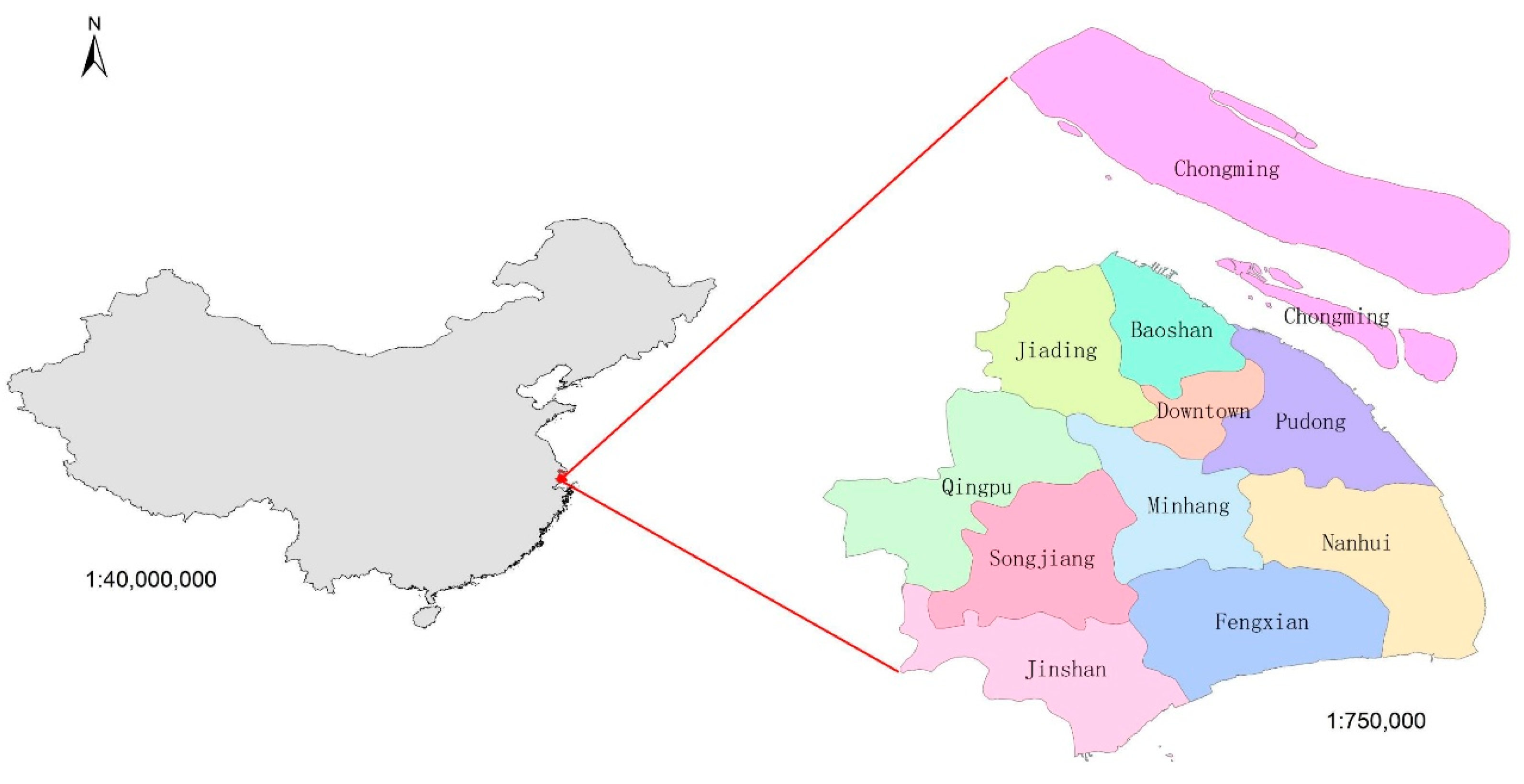
2.1. Study Area
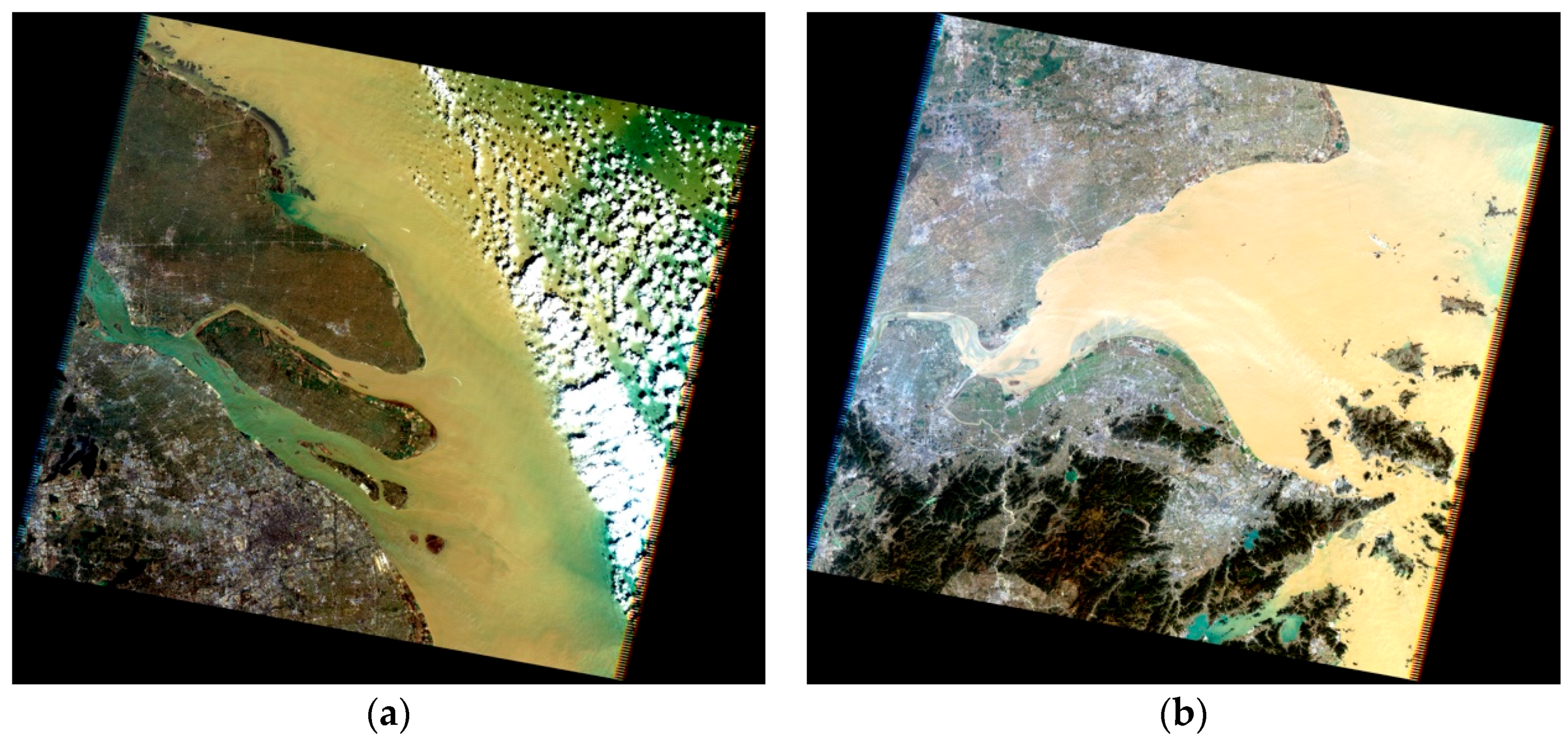
2.2. Image Data
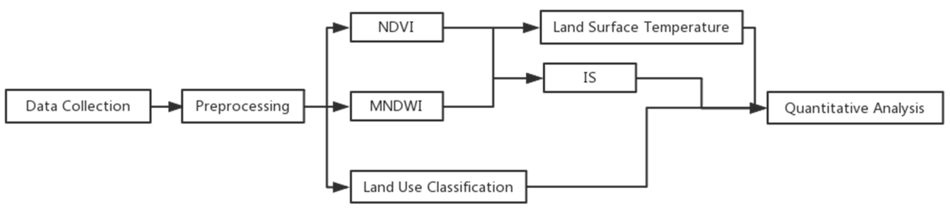
3. Methodology
3.1. Pre-processing
3.1.1. Radiometric Calibration
3.1.2. Atmospheric correction
3.2. Impervious Surface
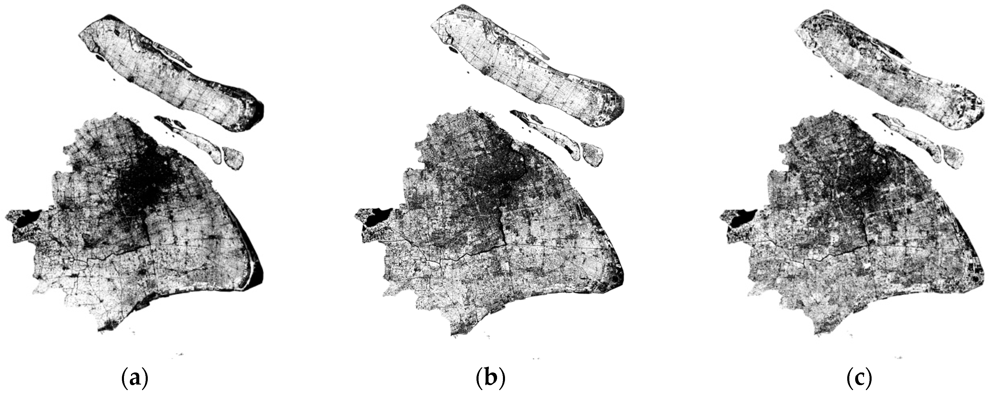
3.2.1. NDVI
3.2.2. MNDWI
3.2.3. Extraction of Impervious Surface
3.3. Land Use Classification
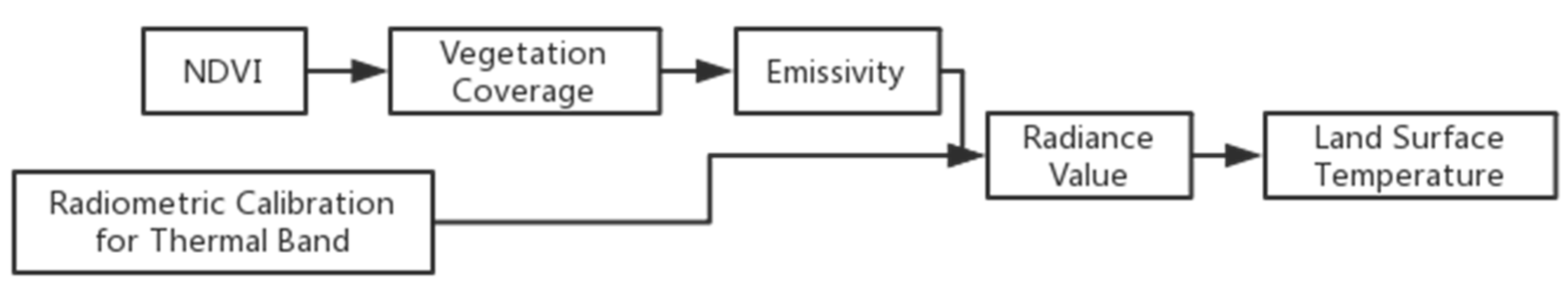
3.4. Land Surface Temperature
4. Experiment
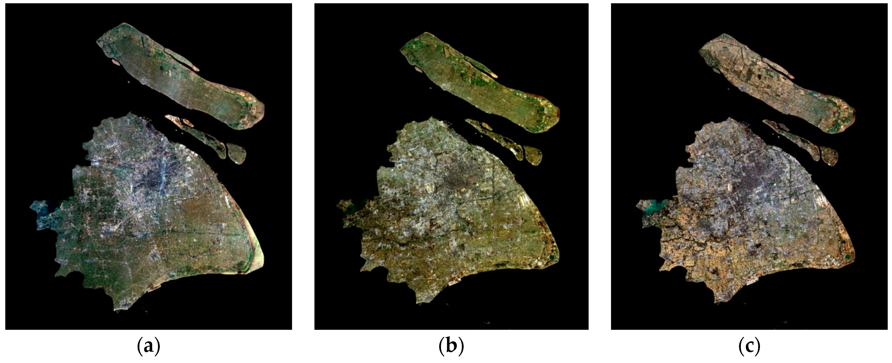
4.1. Preprocessing
4.2. Impervious Surface Extraction
4.2.1. Impervious Surface Calculation
4.2.2. Accuracy Assessment
4.3. Land Use Detection
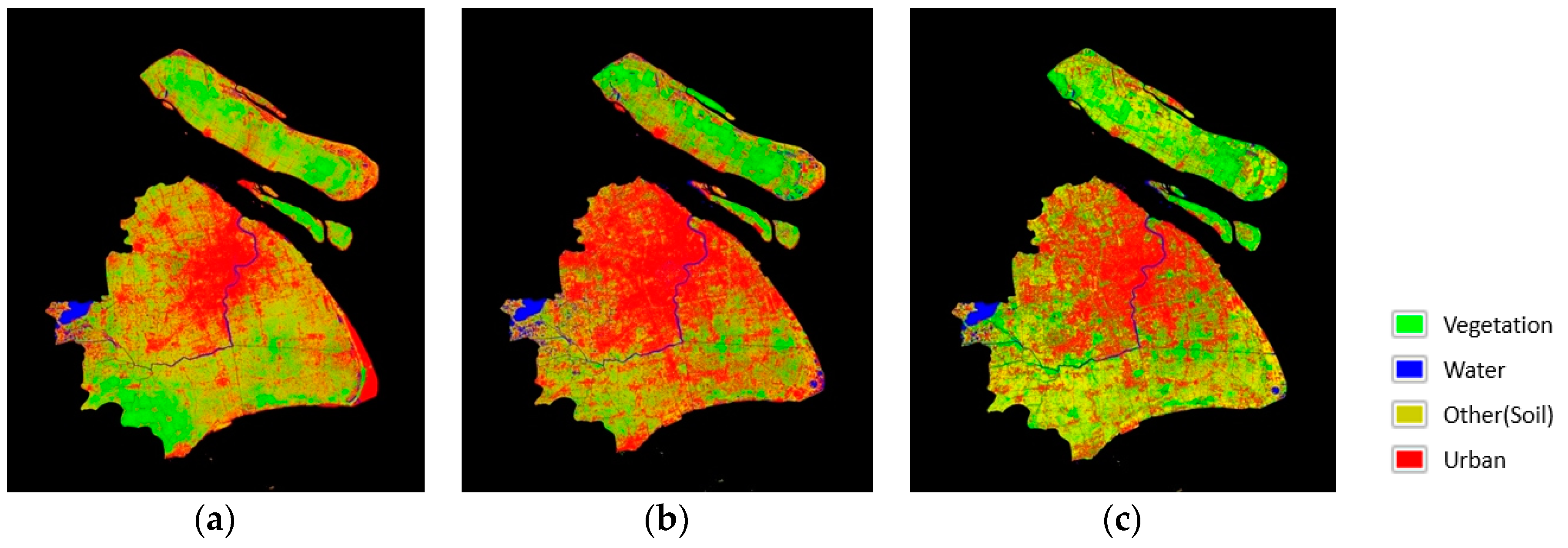
4.3.1. Classification
4.3.2. Confusion Matrix
4.4. Land Surface Temperature Retrieval
4.4.1. Calculation Process
4.4.2. Land Surface Temperature Intervals
5. Results and Analysis
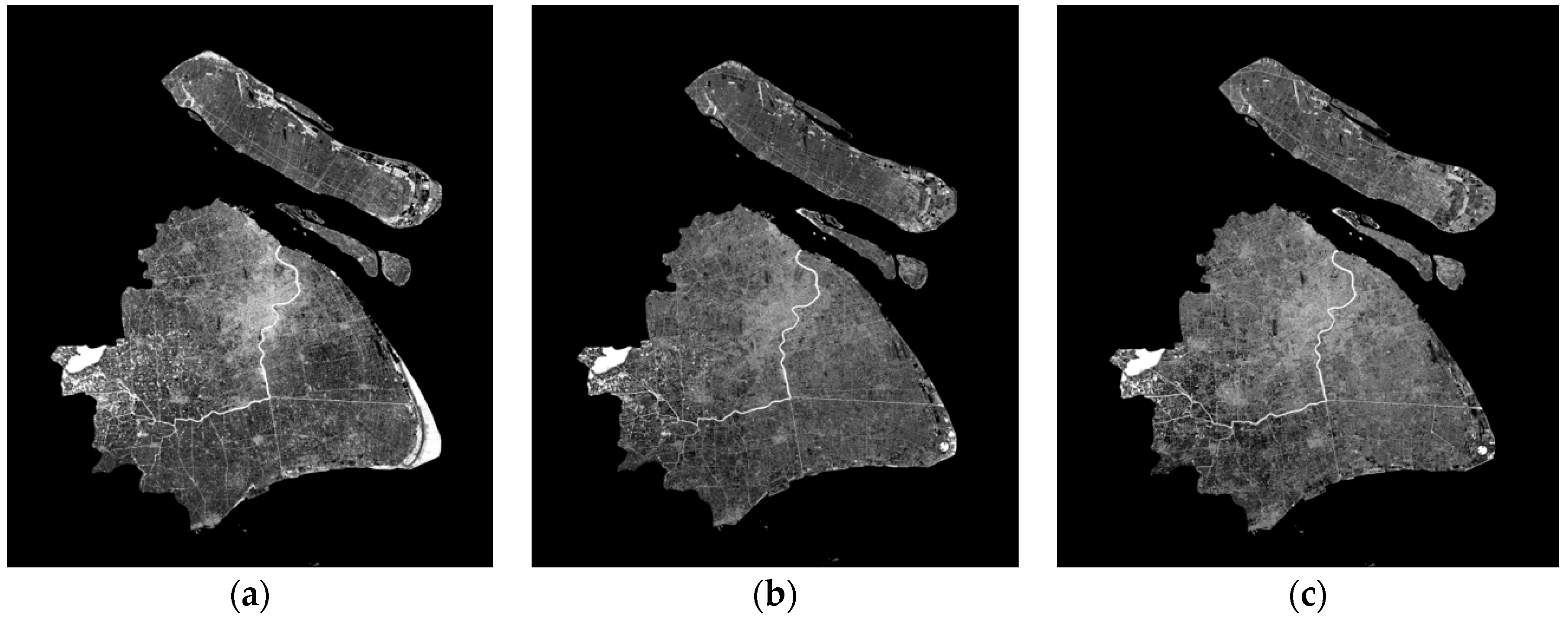
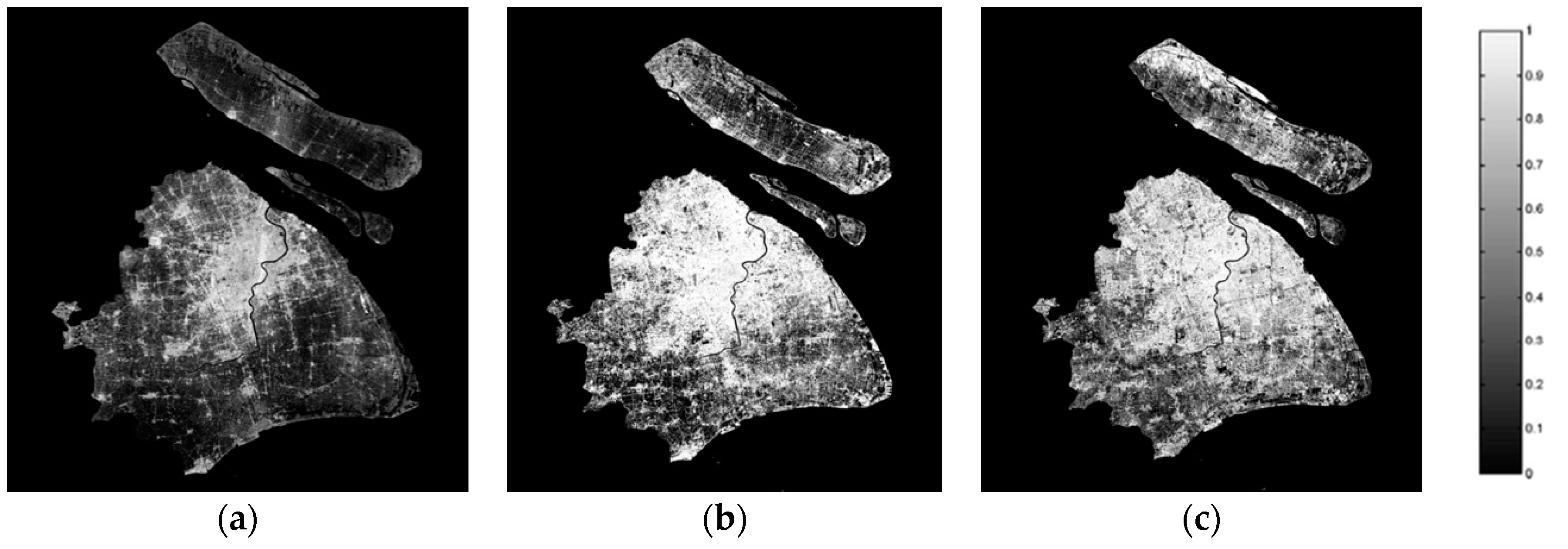
5.1. Spatial Distribution and Characteristics of Impervious Surface
5.1.1. Impervious Surface Distribution in Shanghai
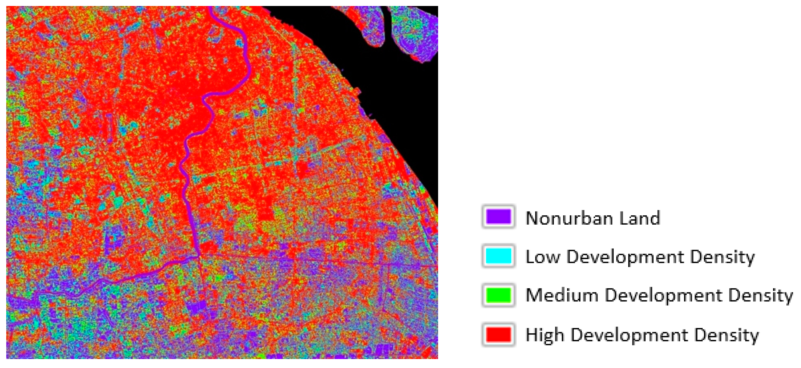
5.1.2. Urban Development Density Analysis
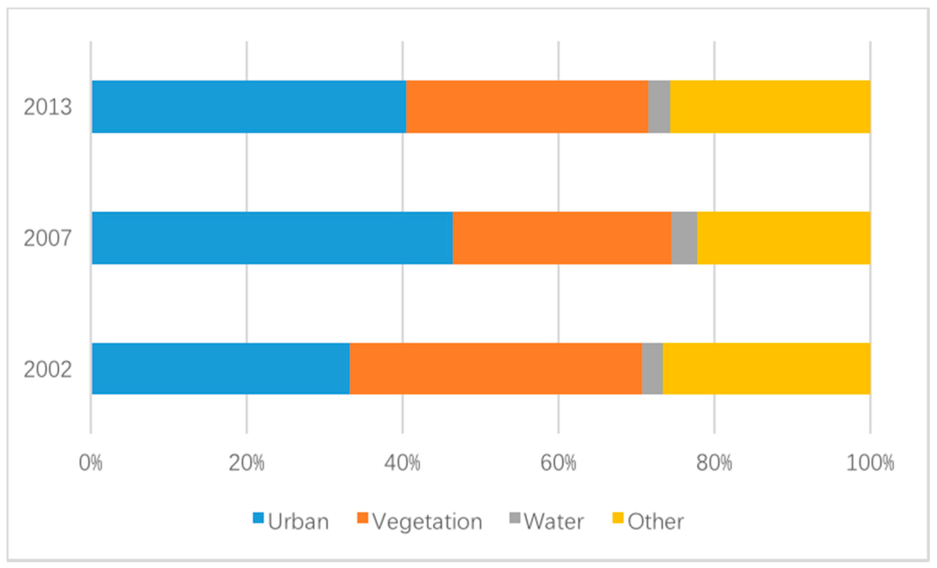
5.2. Land-Use and Land-Cover Change
5.3. Surface Urban Heat Island Analysis
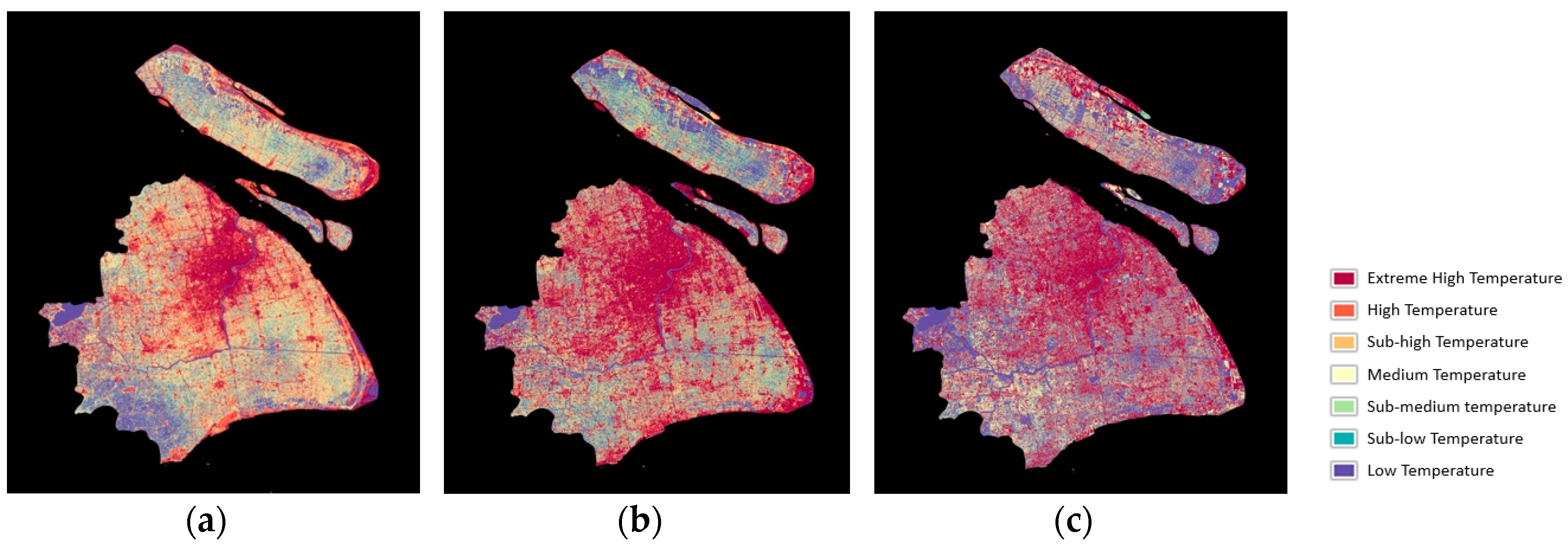
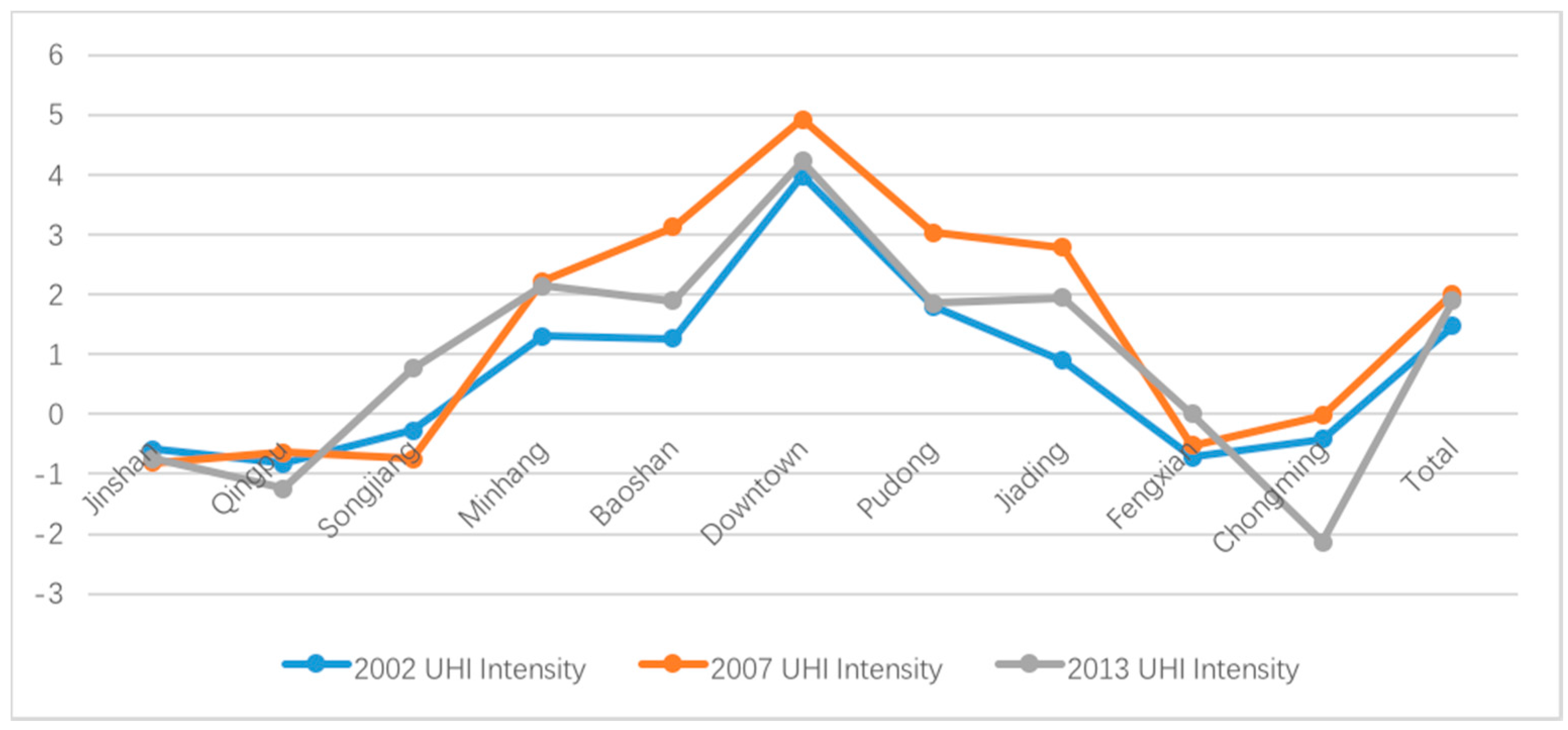
5.3.1. Surface Urban Heat Island Intensity Distribution
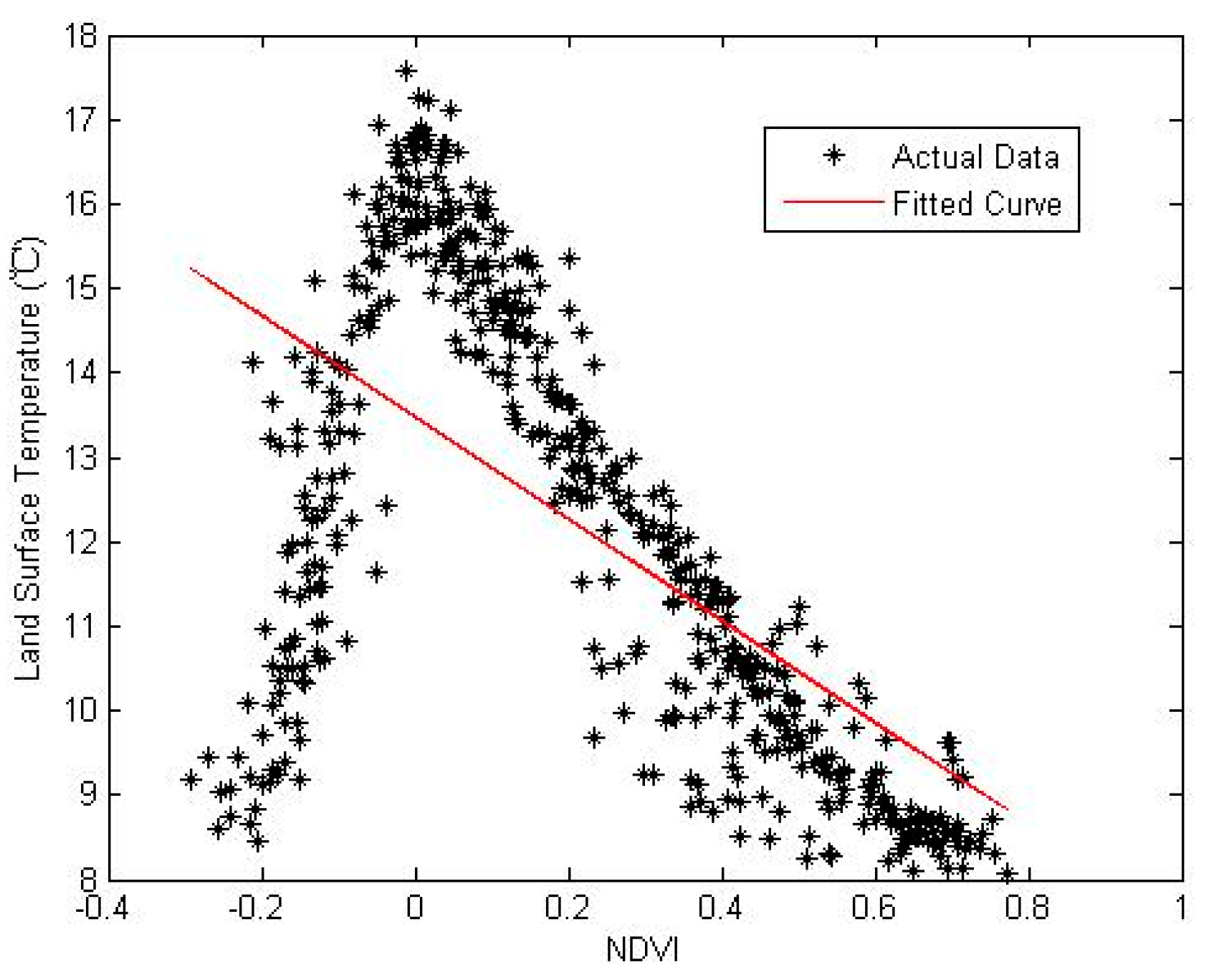
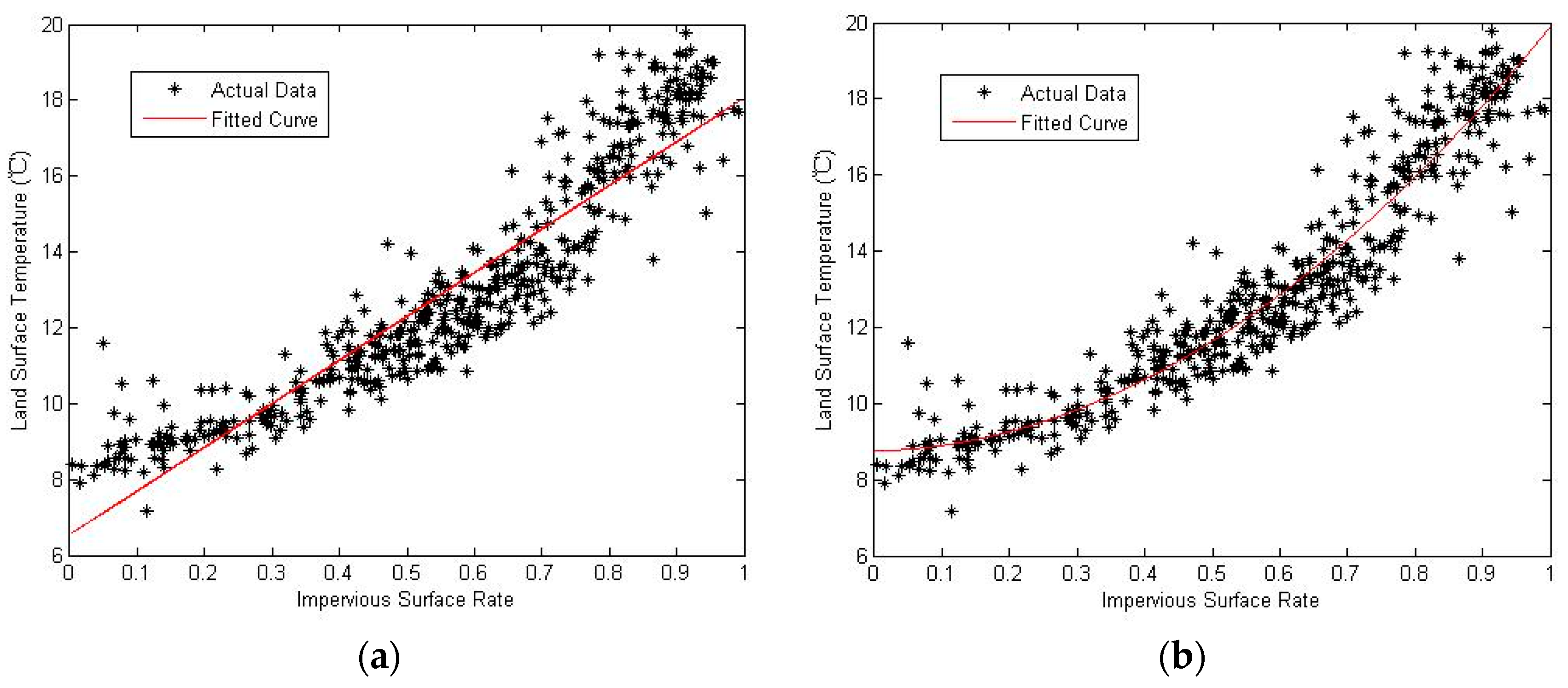
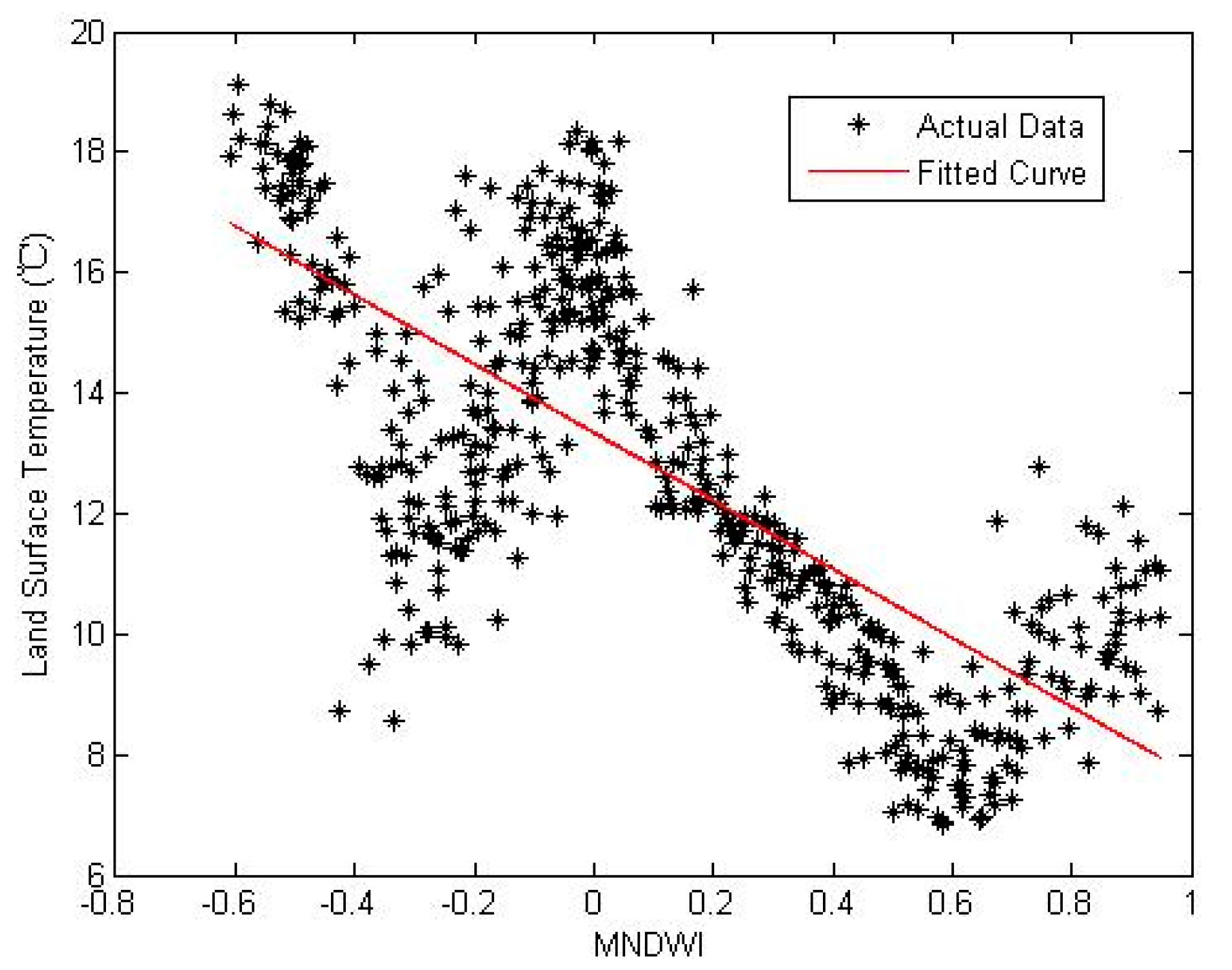
5.3.2. Correlation Analysis of SUHI and IS, LUCC
6. Discussion
7. Conclusions
Acknowledgments
Author Contributions
Conflicts of Interest
References
- Heilig, G.K. World Urbanization Prospects: The 2011 Revision; United Nations, Department of Economic and Social Affairs (DESA), Population Division, Population Estimates and Projections Section: New York, NY, USA, 2012. [Google Scholar]
- Reid, R.S.; Kruska, R.L.; Muthui, N.; Taye, A.; Wotton, S.; Wilson, C.J.; Mulatu, W. Land-use and land-cover dynamics in response to changes in climatic, biological and socio-political forces: The case of southwestern Ethiopia. Landsc. Ecol. 2000, 15, 339–355. [Google Scholar] [CrossRef]
- Huang, J.; Zhao, X.; Tang, L.; Qiu, Q. Analysis on spatiotemporal changes of urban thermal landscape pattern in the context of urbanisation: A case study of Xiamen City. Shengtai Xuebao/Acta Ecol. Sin. 2012, 32, 622–631. [Google Scholar] [CrossRef]
- Alavipanah, S.; Wegmann, M.; Qureshi, S.; Weng, Q.; Koellner, T. The role of vegetation in mitigating urban land surface temperatures: A case study of Munich, Germany during the warm season. Sustainability 2015, 7, 4689–4706. [Google Scholar] [CrossRef]
- Giorgio, G.A.; Ragosta, M.; Telesca, V. Climate variability and industrial-suburban heat environment in a Mediterranean area. Sustainability 2017, 9, 775. [Google Scholar] [CrossRef]
- Wang, J.; Da, L.; Song, K.; Li, B.L. Temporal variations of surface water quality in urban, suburban and rural areas during rapid urbanization in Shanghai, China. Environ. Pollut. 2008, 152, 387–393. [Google Scholar] [CrossRef] [PubMed]
- Cao, K. Analysis of urban rain island effect in shanghai and its changing trend. Water Resour. Power 2009, 5, 31–33. [Google Scholar]
- Kim, H.H. Urban heat island. Int. J. Remote Sens. 1992, 13, 2319–2336. [Google Scholar] [CrossRef]
- Bornstein, R.D. Observations of the urban heat island effect in New York City. J. Appl. Meteorol. 1968, 7, 575–582. [Google Scholar] [CrossRef]
- Magee, N.; Curtis, J.; Wendler, G. The urban heat island effect at Fairbanks, Alaska. Theor. Appl. Climatol. 1999, 64, 39–47. [Google Scholar] [CrossRef]
- Morris, C.J.G.; Simmonds, I.; Plummer, N. Quantification of the influences of wind and cloud on the nocturnal urban heat island of a large city. J. Appl. Meteorol. 2001, 40, 169–182. [Google Scholar] [CrossRef]
- Ackerman, B. Temporal march of the Chicago heat island. J. Clim. Appl. Meteorol. 1985, 24, 547–554. [Google Scholar] [CrossRef]
- Jusuf, S.K.; Wong, N.H.; Hagen, E.; Anggoro, R.; Hong, Y. The influence of land use on the urban heat island in Singapore. Habitat Int. 2007, 31, 232–242. [Google Scholar] [CrossRef]
- Sarkar, H. Study of land cover and population density influences on urban heat island in tropical cities by using remote sensing and GIS: A methodological consideration. In Proceedings of the 3rd FIG Regional Conference, Jakarta, Indonesia, 3–7 October 2004. [Google Scholar]
- Jincai, D.; Zhikai, Z.; Hong, X.; Hongmei, Z. A study of the high temperature distribution and the heat island effect in the summer of the Shanghai area. Chin. J. Atmos. Sci. Chin. Ed. 2002, 26, 420–431. [Google Scholar]
- Yue, W.; Xu, J.; Xu, L. Impact of human activities on urban thermal environment in Shanghai. Acta Geogr. Sin. 2008, 63, 247–256. [Google Scholar]
- Hao, L.P.; Fang, Z.F.; Li, Z.L.; Liu, Z.Q.; He, J.H. The inter-annual climate change and heat island effect of Chengdu during the recent fifty years. Sci. Meteor. Sin. 2007, 27, 648–654. [Google Scholar]
- Yang, B. Progress of urban heat island effect. J. Meteorol. Environ. 2013, 2, 101–106. [Google Scholar]
- Bai, Z.P.; Qi, T. Monitoring “heat island effect” in urban regions. Cities Disaster Reduct. 2004, 2, 27–28. [Google Scholar]
- Zhao, K.X. Current situation and countermeasures of urban heat island effect. Chin. Landsc. Archit. 1999, 6, 44–45. [Google Scholar]
- Wang, G.X.; Shen, X.L. On the relationship between urbanization and heat island effect in Shanghai. J. Subtrop. Res. Environ. 2010, 5, 1–11. [Google Scholar]
- Chen, X.L.; Zhao, H.M.; Li, P.X.; Yin, Z.Y. Remote sensing image-based analysis of the relationship between urban heat island and land use/cover changes. Remote Sens. Environ. 2006, 104, 133–146. [Google Scholar] [CrossRef]
- Weng, Q.; Lu, D.; Schubring, J. Estimation of land surface temperature–vegetation abundance relationship for urban heat island studies. Remote Sens. Environ. 2004, 89, 467–483. [Google Scholar] [CrossRef]
- Sailor, D.J. Simulated urban climate response to modifications in surface albedo and vegetative cover. J. Appl. Meteorol. 1995, 34, 1694–1704. [Google Scholar] [CrossRef]
- Arnfield, A.J. Two decades of urban climate research: A review of turbulence, exchanges of energy and water, and the urban heat island. Int. J. Climatol. 2003, 23, 1–26. [Google Scholar] [CrossRef]
- Yuan, F.; Bauer, M.E. Comparison of impervious surface area and normalized difference vegetation index as indicators of surface urban heat island effects in Landsat imagery. Remote Sens. Environ. 2007, 106, 375–386. [Google Scholar] [CrossRef]
- Zhou, Y.; Shi, T.M.; Yuan-Man, H.U.; Gao, C.; Liu, M. Relationships between land surface temperature and normalized difference vegetation index based on urban land use type. Chin. J. Ecol. 2011, 30, 1504–1512. [Google Scholar]
- Xu, H.Q. Quantitative analysis on the relationship of urban impervious surface with other components of the urban ecosystem. Acta Ecol. Sin. 2009, 29, 2456–2462. [Google Scholar]
- Lin, Y.S.; Xu, H.Q.; Zhou, R. A study on urban impervious surface area and its relation with urban heat island: Quanzhou city, China. Remote Sens. Technol. Appl. 2007, 22, 14–19. [Google Scholar]
- Cao, L.; Hu, W.H.; Meng, X.L.; Li, J.X. Relationships between land surface temperature and key landscape elements in urban area. Chin. J. Ecol. 2011, 30, 2329–2334. [Google Scholar]
- Mu, H.Z.; Kong, C.Y.; Tang, X.; Ke, X.X. Preliminary analysis of temperature change in Shanghai and urbanization impacts. J. Trop. Meteorol. 2008, 24, 673–674. [Google Scholar]
- Li, D.; Bou-Zeid, E. Quality and sensitivity of high-resolution numerical simulation of urban heat islands. Environ. Res. Lett. 2014, 9, 055001. [Google Scholar] [CrossRef]
- Voogt, J.A.; Oke, T.R. Thermal remote sensing of urban climates. Remote Sens. Environ. 2003, 86, 370–384. [Google Scholar] [CrossRef]
- Quattrochi, D.A.; Luvall, J.C.; Rickman, D.L.; Estes, M.G.; Laymon, C.A.; Howell, B.F. A decision support information system for urban landscape management using thermal infrared data: Decision support systems. Photogramm. Eng. Remote Sens. 2000, 66, 1195–1207. [Google Scholar]
- Picón, A.J.; Vásquez, R.; González, J.; Luvall, J.; Rickman, D. Use of remote sensing observations to study the urban climate on tropical coastal cities. Rev. Umbral (Etapa IV Colecc. Complet.) 2017, 1, 218–232. [Google Scholar]
- EnergyPlus. Available online: https://energyplus.net/weather-location/asia_wmo_region_2/CHN/ (accessed on 25 May 2017).
- United States Geological Survey. Available online: https://www.usgs.gov (accessed on 3 April 2017).
- Zhou, J.Q.; Ye, Q.; Shao, Y.S.; Zhu, S.L.; Guan, Z.Q. Principles and Application of Remote Sensing; Wuhan University Press: Wuhan, China, 2014. [Google Scholar]
- McFeeters, S.K. The use of the Normalized Difference Water Index (NDWI) in the delineation of open water features. Int. J. Remote Sens. 1996, 17, 1425–1432. [Google Scholar] [CrossRef]
- Xu, H. A study on information extraction of water body with the modified normalized difference water index (MNDWI). J. Remote Sens. 2005, 9, 589–595. [Google Scholar]
- Leprieur, C.; Verstraete, M.M.; Pinty, B. Evaluation of the performance of various vegetation indices to retrieve vegetation cover from AVHRR data. Remote Sens. Rev. 1994, 10, 265–284. [Google Scholar] [CrossRef]
- Kim, H.; Loh, W.Y. Classification trees with unbiased multiway splits. J. Am. Stat. Assoc. 2001, 96, 589–604. [Google Scholar] [CrossRef]
- Jiménez-Muñoz, J.C.; Sobrino, J.A.; Skoković, D.; Mattar, C.; Cristóbal, J. Land surface temperature retrieval methods from Landsat-8 thermal infrared sensor data. IEEE Geosci. Remote Sens. Lett. 2014, 11, 1840–1843. [Google Scholar] [CrossRef]
- Copertino, V.A.; Pierro, M.D.; Scavone, G.; Telesca, V. Comparison of algorithms to retrieve lst from LANDSAT-7 ETM+ IR data in the Basilicata Ionian band. Tethys J. Weather Clim. West. Mediterr. 2002, 25–34. [Google Scholar]
- Sobrino, J.A.; Jiménez-Muñoz, J.C.; Paolini, L. Land surface temperature retrieval from LANDSAT TM 5. Remote Sens. Environ. 2004, 90, 434–440. [Google Scholar] [CrossRef]
- Jiménez-Muñoz, J.C.; Sobrino, J.A. A generalized single-channel method for retrieving land surface temperature from remote sensing data. J. Geophys. Res. Atmos. 2003, 108, 2015–2023. [Google Scholar] [CrossRef]
- Zhang, X.; Zhu, Q.J.; Min, X.J. Analysis of split window algorithms for estimating land surface temperature from AVHRR data. J. Image Gr. 1999, 4, 595–599. [Google Scholar]
- Prata, A.J. Land surface temperatures derived from the advanced very high resolution radiometer and the along-track scanning radiometer. J. Geophys. Res. Atmos. 1993, 981, 16689–16702. [Google Scholar] [CrossRef]
- Sobrino, J.A.; Li, Z.; Stoll, M.P.; Becker, F. Multi-channel and multi-angle algorithms for estimating sea and land surface temperature with ATSR data. Int. J. Remote Sens. 1996, 17, 2089–2114. [Google Scholar] [CrossRef]
- Ding, F.; Xu, H.Q. Comparison of three algorithms for retrieving land surface temperature from LANDSAT TM thermal infrared band. J. Fujian Normal Univ. (Nat. Sci. Ed.) 2008, 24, 91–96. [Google Scholar]
- Xian, G.; Crane, M. An analysis of urban thermal characteristics and associated land cover in Tampa Bay and Las Vegas using Landsat satellite data. Remote Sens. Environ. 2006, 104, 147–156. [Google Scholar] [CrossRef]
- Zhang, Y.; Bao, W.J.; Qi, Y.U. Study on seasonal variations of the urban heat island and its interannual changes in a typical Chinese megacity. Chin. J. Geophys. 2012, 55, 1121–1128. [Google Scholar]
- Shanghai Municipal Statistics Bureau. 2017. Available online: http://www.stats-sh.gov.cn/frontinfo/staticPageView.xhtml?para=ldcy (accessed on 25 May 2017).


| Jan | Feb | Mar | Apr | May | Jun | Jul | Aug | Sep | Oct | Nov | Dec | |
|---|---|---|---|---|---|---|---|---|---|---|---|---|
| Avg Temp. (℃) | 4 | 5 | 8 | 14 | 19 | 24 | 28 | 27 | 23 | 18 | 12 | 7 |
| Wind Direction (°) | 290 | 40 | 0 | 110 | 90 | 110 | 150 | 140 | 60 | 20 | 20 | 290 |
| Wind Speed (m/s) | 2 | 3 | 3 | 3 | 3 | 2 | 4 | 2 | 3 | 2 | 3 | 2 |
| Relative Humidity | 73 | 78 | 73 | 76 | 81 | 83 | 79 | 77 | 82 | 75 | 73 | 70 |
| Global Horiz Radiation (Avg Daily Total, Wh/sq.m) | 2131 | 2362 | 2791 | 4041 | 4119 | 4003 | 4782 | 5061 | 3257 | 3338 | 2533 | 2316 |
| Avg precipitation (mm) | 74.4 | 59.1 | 93.8 | 74.2 | 84.5 | 181.8 | 145.7 | 213.7 | 87.1 | 55.6 | 52.3 | 43.9 |
| File Name | 2002003 | 2007033 | 2013337 |
|---|---|---|---|
| Location | Shanghai | ||
| Sensor | Landsat5 TM | Landsat5 TM | Landsat8 OLI |
| Spatial | 30 × 30 m | ||
| Temporal | 3 January 2002 | 2 February 2007 | 3 December 2013 |
| Spectral (micrometers) | Band 1 = Blue (0.45–0.52) Band 2 = Green (0.52–0.6) Band 3 = Red (0.63–0.69) Band 4 = NIR (0.76–0.9) Band 5 = SWIR (1.55–1.75) Band 6 = TIR (10.4–12.5) * Band 7 = SWIR (2.08–2.35) | Band 1 = Blue (0.45–0.52) Band 2 = Green (0.52–0.6) Band 3 = Red (0.63–0.69) Band 4 = NIR (0.76–0.9) Band 5 = SWIR (1.55–1.75) Band 6 = TIR (10.4–12.5) * Band 7 = SWIR (2.08–2.35) | Band 1 = Coastal (0.433–0.453) Band 2 = Blue (0.450–0.515) Band 3 = Green (0.525–0.6) Band 4 = Red (0.630–0.680) Band 5 = NIR (0.845–0.885) Band 6 = SWIR 1 (1.560–1.660) Band 7 = SWIR 2 (2.100–2.300) Band 8 = Pan (0.500–0.680) * Band 9 = Cirrus (1.360–1.390) Band 10 = TIRS 1 (10.6–11.2) * Band 11 = TIRS 2 (12.0–12.5) * |
| Year | 2002 | 2009 | 2013 |
|---|---|---|---|
| Percentage | 19.47% | 36.23% | 37.09% |
| Area (km2) | 1234.40 | 2296.98 | 2351.56 |
| Year | 2002 | 2009 | 2013 |
|---|---|---|---|
| Accuracy | 90.50% | 87.79% | 89.34% |
| Year | 2002 | 2009 | 2013 |
|---|---|---|---|
| Overall Accuracy | 85.59% | 83.20% | 88.14% |
| Kappa Coefficient | 0.7874 | 0.7536 | 0.8117 |
| Temperature Grade | Range |
|---|---|
| Extreme high temperature | |
| High temperature | |
| Sub-high temperature | |
| Medium temperature | |
| Sub-medium temperature | |
| Sub-low temperature | |
| Low temperature |
| Downtown | Pudong | Minhang | Baoshan | Jiading | |
| 2002 | 160.87 | 217.63 | 126.59 | 148.41 | 86.71 |
| 2007 | 242.64 | 528.73 | 230.77 | 210.64 | 216.13 |
| 2013 | 238.95 | 544.71 | 231.06 | 216.39 | 216.70 |
| Jinshan | Songjiang | Qingpu | Fengxian | Chongming | |
| 2002 | 35.93 | 64.15 | 69.78 | 50.41 | 177.92 |
| 2007 | 111.27 | 165.76 | 155.06 | 194.93 | 241.05 |
| 2013 | 112.86 | 180.09 | 155.64 | 196.77 | 258.39 |
| Downtown | Pudong | Minhang | Baoshan | Jiading | |
| 2002 | 55.66% | 17.98% | 34.03% | 49.47% | 18.89% |
| 2007 | 83.95% | 43.69% | 62.03% | 70.21% | 47.08% |
| 2013 | 82.68% | 45.02% | 62.11% | 72.13% | 47.21% |
| Jinshan | Songjiang | Qingpu | Fengxian | Chongming | |
| 2002 | 6.13% | 10.60% | 10.32% | 7.34% | 15.01% |
| 2007 | 18.99% | 27.39% | 22.94% | 28.37% | 20.34% |
| 2013 | 19.26% | 29.76% | 23.02% | 28.64% | 21.80% |
| Downtown | Pudong | Minhang | Baoshan | Jiading | |
| 2002–2007 | 81.77 | 311.10 | 104.18 | 62.23 | 129.42 |
| 2007–2013 | −3.69 | 15.98 | 0.29 | 5.75 | 0.57 |
| Total | 78.08 | 327.08 | 104.47 | 67.98 | 129.99 |
| Jinshan | Songjiang | Qingpu | Fengxian | Chongming | |
| 2002–2007 | 75.34 | 101.61 | 85.28 | 144.52 | 63.13 |
| 2007–2013 | 1.59 | 14.33 | 0.58 | 1.84 | 17.34 |
| Total | 76.93 | 115.94 | 85.86 | 146.36 | 80.47 |
| Downtown | Pudong | Minhang | Baoshan | Jiading | |
| 2002–2007 | 50.83% | 142.95% | 82.29% | 41.93% | 149.25% |
| 2007–2013 | −1.52% | 3.02% | 0.126% | 2.73% | 0.264% |
| Jinshan | Songjiang | Qingpu | Fengxian | Chongming | |
| 2002–2007 | 209.68% | 158.39% | 122.21% | 286.68% | 35.48% |
| 2007–2013 | 1.43% | 8.65% | 0.374% | 0.944% | 7.19% |
| Urban | Vegetation | Water | Other | |
|---|---|---|---|---|
| 2002 | 2105.96 | 2375.86 | 165.64 | 1692.84 |
| 2007 | 2940.93 | 1785.94 | 202.10 | 1413.76 |
| 2013 | 2562.84 | 1973.15 | 175.39 | 1629.98 |
| 2002 Avg Temp. | 2002 UHI Intensity | 2007 Avg Temp. | 2007 UHI Intensity | 2013 Avg Temp. | 2013 UHI Intensity | |
|---|---|---|---|---|---|---|
| Jinshan | 7.697 | −0.586 | 10.736 | −0.806 | 10.436 | −0.753 |
| Qingpu | 7.459 | −0.824 | 10.908 | −0.638 | 9.974 | −1.246 |
| Songjiang | 8.084 | −0.274 | 10.813 | −0.742 | 11.942 | 0.764 |
| Minhang | 9.577 | 1.297 | 13.647 | 2.217 | 14.145 | 2.135 |
| Baoshan | 9.485 | 1.266 | 14.636 | 3.122 | 13.746 | 1.894 |
| Downtown | 12.192 | 3.978 | 16.135 | 4.914 | 15.864 | 4.217 |
| Pudong | 9.997 | 1.797 | 14.742 | 3.033 | 12.798 | 1.853 |
| Jiading | 9.096 | 0.897 | 14.126 | 2.783 | 13.120 | 1.935 |
| Fengxian | 7.437 | −0.721 | 11.063 | −0.523 | 11.752 | −0.004 |
| Chongming | 7.765 | −0.416 | 11.130 | −0.024 | 8.969 | −2.131 |
| Total | 8.846 | 1.463 | 11.837 | 2.012 | 11.033 | 1.894 |
© 2017 by the authors. Licensee MDPI, Basel, Switzerland. This article is an open access article distributed under the terms and conditions of the Creative Commons Attribution (CC BY) license (http://creativecommons.org/licenses/by/4.0/).
Share and Cite
Wang, H.; Zhang, Y.; Tsou, J.Y.; Li, Y. Surface Urban Heat Island Analysis of Shanghai (China) Based on the Change of Land Use and Land Cover. Sustainability 2017, 9, 1538. https://doi.org/10.3390/su9091538
Wang H, Zhang Y, Tsou JY, Li Y. Surface Urban Heat Island Analysis of Shanghai (China) Based on the Change of Land Use and Land Cover. Sustainability. 2017; 9(9):1538. https://doi.org/10.3390/su9091538
Chicago/Turabian StyleWang, Haiting, Yuanzhi Zhang, Jin Yeu Tsou, and Yu Li. 2017. "Surface Urban Heat Island Analysis of Shanghai (China) Based on the Change of Land Use and Land Cover" Sustainability 9, no. 9: 1538. https://doi.org/10.3390/su9091538
APA StyleWang, H., Zhang, Y., Tsou, J. Y., & Li, Y. (2017). Surface Urban Heat Island Analysis of Shanghai (China) Based on the Change of Land Use and Land Cover. Sustainability, 9(9), 1538. https://doi.org/10.3390/su9091538