Analysis of Total Factor Efficiency of Water Resource and Energy in China: A Study Based on DEA-SBM Model

Abstract

One of the serious issues that China faces during its fast economic development is the low input–output efficiency of water and energy resources and growing water pollution. With the current economic development model of China, economic growth still requires large input of water resource and energy resource. This paper has focused on the total factor efficiency of water resource and energy resource by each province in China. We treat the undesirable outputs as outputs in the DEA-SBM Model instead of as inputs in previous studies, and design a new MATLAB programming to achieve optimization solutions of multi-variable constrained nonlinear functions to evaluate the Total Factor Efficiency of Water resource (TFEW) and the Total Factor Efficiency of Energy (TFEE) in China accurately. By using the method, this paper has analyzed the TFEW and TFEE in China from 2003 to 2014 by economic zones and typical provinces and provided corresponding policy recommendations.

1. Introduction

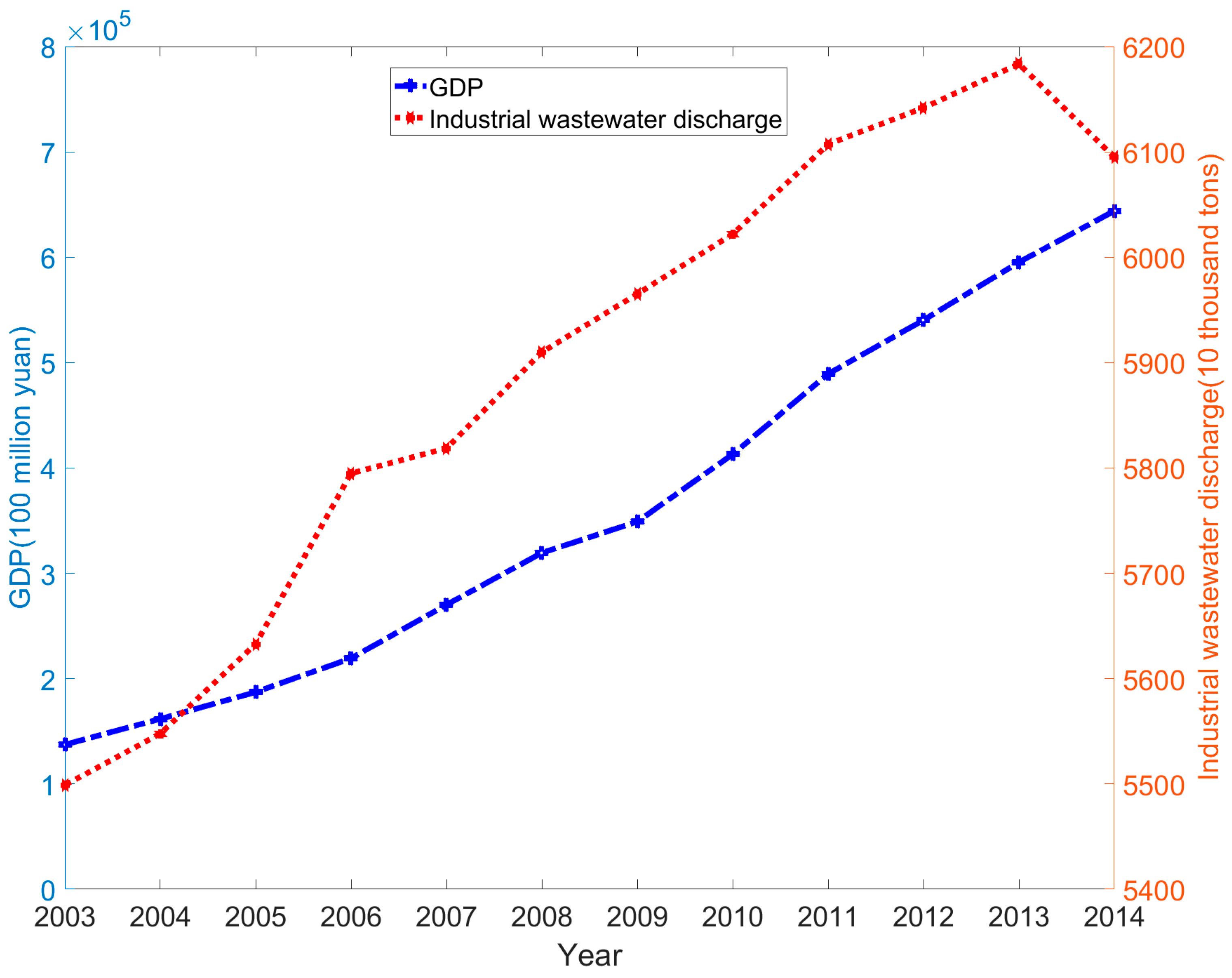
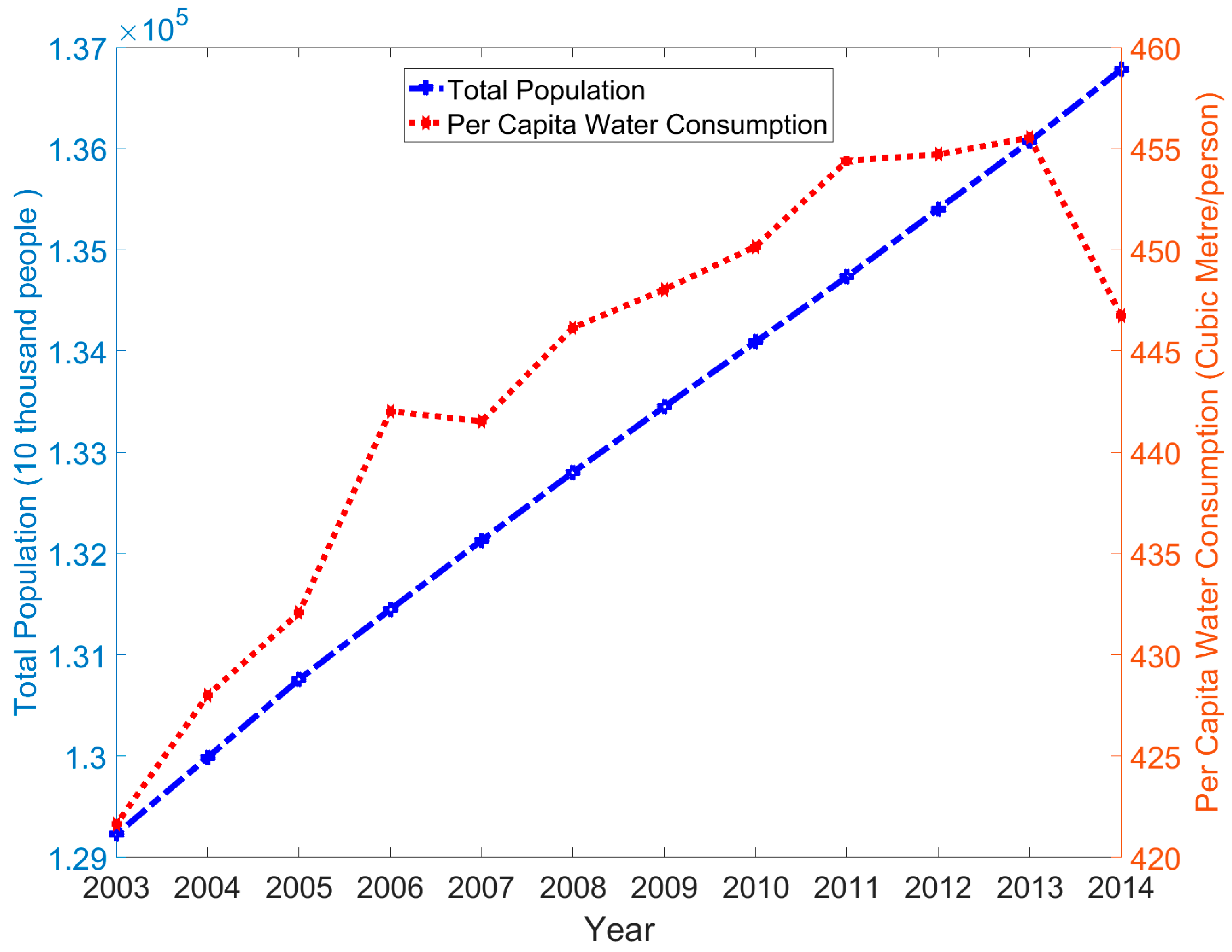
Water is not only a crucial resource for the survival of mankind, it is also a strategic resource for the development of human society. Because of the reform and opening-up, China has achieved fast economic growth along with growing water resource consumption (see Figure 1) [1].

Although water is the crucial basis for human survival and development, China is not rich in water resource. The nation’s average water resource per unit area is only 299 thousand m³/km², around 83% of the world’s average level. However, China’s per capita water resource consumption has been above 440 m³/person since 2006, which becomes an increasingly heavy burden (see Figure 2) [1].

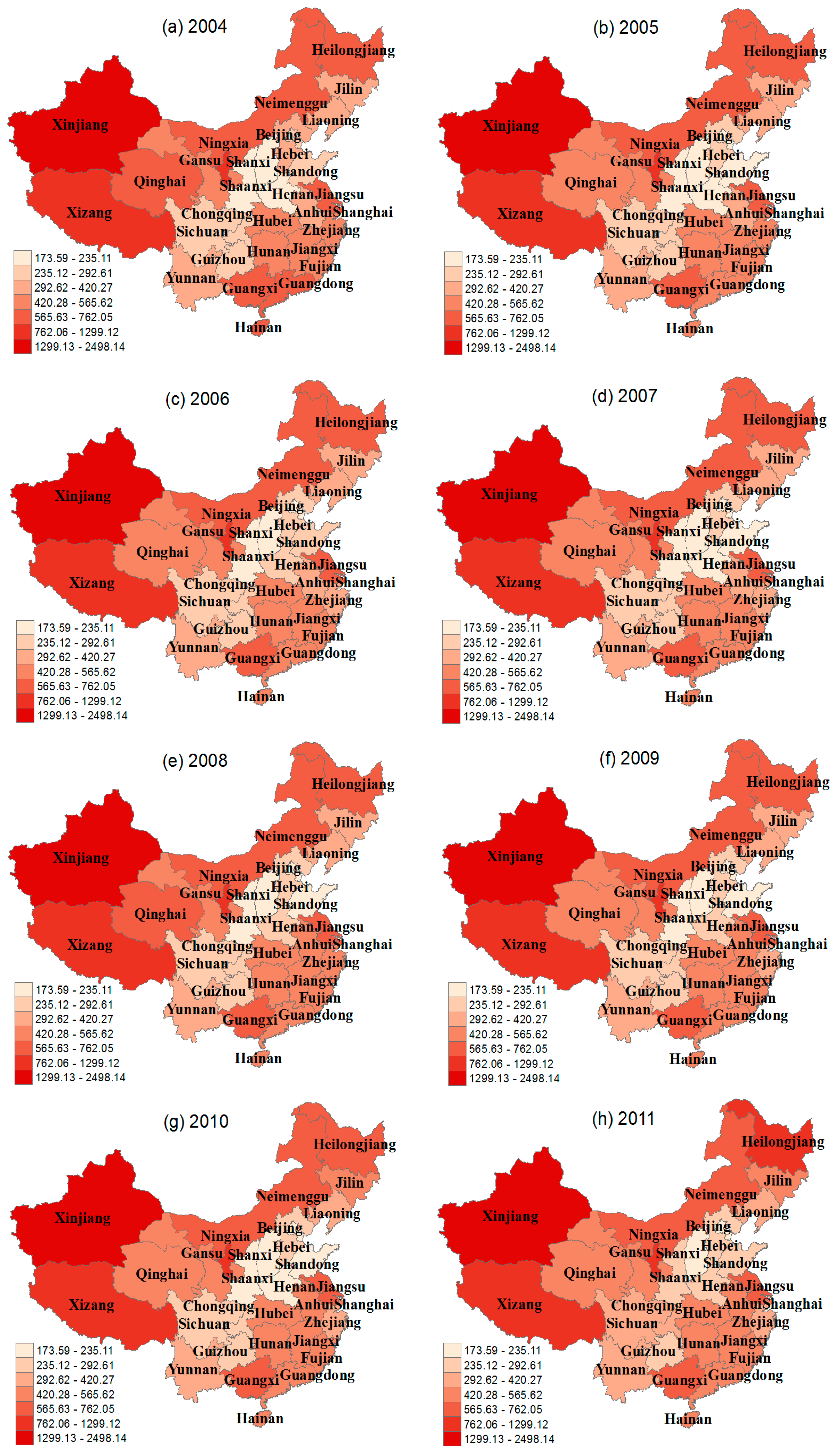
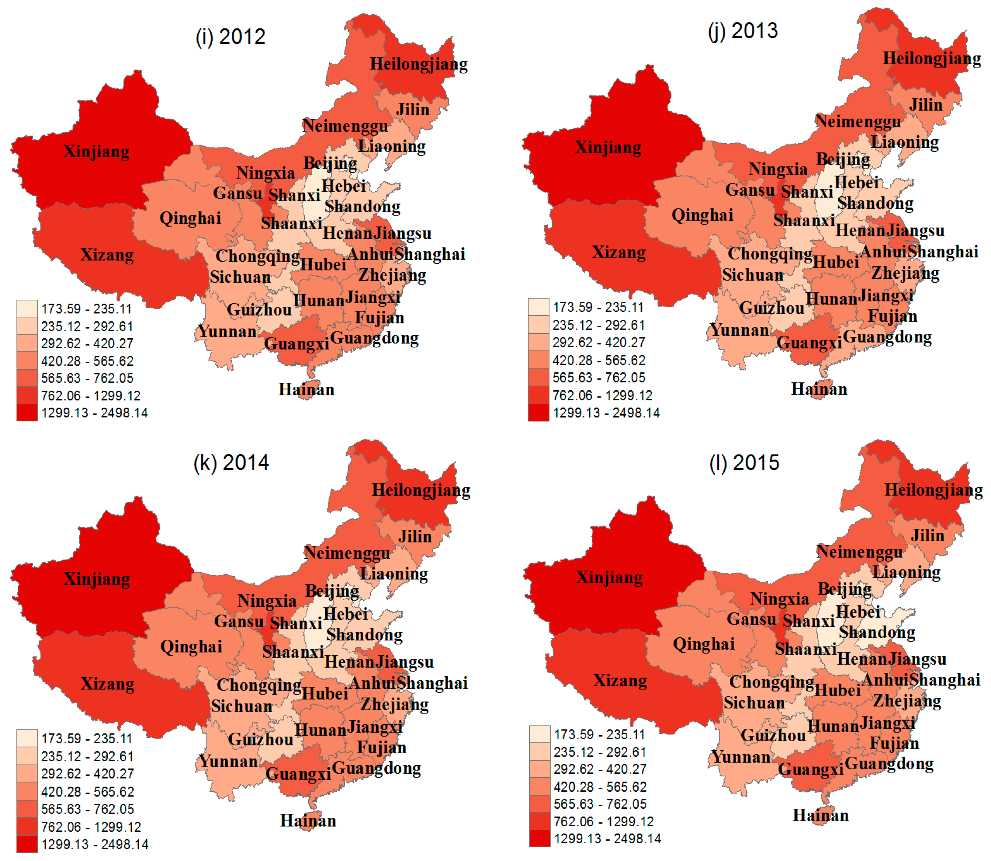
Moreover, the temporal and spatial distributions of provincial per capita water resource consumption of China are very unbalanced, which cannot match well with the farmland resource and other economic factors. In addition, the construction of China’s hydraulic project system is still not perfect. Thus, the conflict between supply and demand of water resources is becoming increasingly acute in north, northwest, southwest and coastal cities in China (see Figure 3) [2].

In fact, both the central government and local governments of all levels have highly emphasized the importance of water resource. In 2011, the first administration document issued by the Chinese Central Committee of the Communist Party and the State Council was about the speeding up of hydraulic reform in China. In this “No. 1 Document”, the central government clearly stated that in order to strengthen water resource management and improve factor efficiency in both industrial and agricultural utilization of water resource, we must draw a red line in water efficiency by 2020: (1) building the reasonable allocation and high-efficient utilization system of water resource; (2) keeping the annual national total water consumption below 670 billion m³; (3) significantly improving the urban and rural water supply ratio, and fully protecting drinking water safety for urban and rural residents; and (4) increasing the effective utilization coefficient of farmland irrigation water equal to or greater than 0.55 [3].

Current academic studies mainly focus on the efficiency of water utilization in China. Wang and Lu (2014) studied the regional difference in efficiency of water utilization in agriculture [4]. Han et al. (2016) studied the footprint of grey water across different provinces, its efficiency and development patterns [5]. However, apart from the efficiency of water utilization as well as its constraints on China’s economic development, we must also pay attention to another crucial aspect: the large-volume emissions of wastewater along with serious water pollution during the process of manufacture and economic development.

By focusing our study on the efficiency of China’s water resource, we must answer these two questions from a quantitatively aspect: What is the input–output efficiency of water resource as a production factor? How should the effect of undesirable outputs such as wastewater generated during the production process be measured? We consider the second question because the pollution of wastewater discharge to existing water resources can be controlled by reducing the wastewater as an undesirable output. In 2014, China’s total discharge of wastewater amounted to 71.62 billion tons, which contains 73,184.74 kg lead, 745.91 kg mercury, and 17,251.10 kg cadmium [2]. These pollutants entered the water or soil and further increased the level of water and soil pollution [6]. This situation also pushed the government and the enterprises to use emission reduction technologies widely. Li et al. (2017) take the textile industry in China as an example. They find that with emission reduction technologies, the textile industry increase water reuse rate of 15% to over 30% at the end of 2015 [7]. Therefore, it will help to relieve the water shortage pressure faced by China.

As for the second question, the common practice in academic literature is to treat the undesirable outputs (such as pollution) as input factors in production functions. Although this could greatly simplify the model setting and calculation process, it did not treat pollution as an output or result of the production process. Hence, this method did not exactly match the fundamental structure of the production model, and would result in certain deviation from the reality.

Therefore, based on the theoretical discussion and empirical studies on water efficiency, this paper has considered the features of water resources in China as well as its utilization efficiency in different provinces, and constructed a comprehensive research system on water efficiency and sustainable development of China. In the following parts, Section 2 will systematically review major literature on water efficiency. By introducing the undesirable outputs into the Data Envelope Analysis (DEA) Model commonly adopted by similar studies, Section 3 will set up a model to achieve maximum output with minimum undesirable outputs. Based on the innovative MATLAB programming designed by us, Section 4 will quantitatively calculate and analyze the utilization efficiency of water resource in different provinces and economic zones of China under the assumption of maximum output with minimum undesirable outputs, and discuss possible reasons for the difference across different regions. Finally, Section 5 will provide conclusion on overall findings of this study and related policy recommendations.

2. Literature Review

In terms of the development of academic studies on water efficiency, it has been through early stages of study on production efficiency and consumption efficiency, and now reached the stage of overall productivity of water resources as well as overall economic efficiency study covering all kinds of output factors. The early stage studies mainly focused on one of the traditional usages of water resource in agriculture: irrigation. Choudhury and Kumar (1980) have analyzed the growth and yield of wheat with different water pressures during irrigation in order to find the optimal irrigation water pressure to achieve certain wheat yields [8]. Barker et al. (2000) have differentiated irrigation efficiency into water transmission efficiency and field utilization efficiency. They pointed out that a high irrigation efficiency may not be able to ensure a high water resource utilization efficiency or management skills [9]. Kaneko et al. (2004) have used the Cobb–Douglas Production Function to assess the irrigation efficiency of water resource [10]. By calculating the irrigation efficiency of water resource in different provinces of China from 1999 to 2002, they have concluded that the main factors that impacts irrigation efficiency of agriculture include natural factors (such as climate, soil, etc.) and infrastructure (such as farmland construction, irrigation facilities, etc.) Based on the cross-sectional survey data of farmers, Speelman et al. (2007) have calculated the irrigation efficiency under different scales of economy. Their study shows that factors including land ownership, agricultural acreage, irrigation technology, different types of crops and their plantation structures will all have impacts on the irrigation efficiency [11].

With the development of research in this field, academic studies on water efficiency have gradually expanded from the traditional irrigation usage in agriculture to the entire agriculture and the overall input–output structure of the national economy. Based on their calculation result of water efficiency in agriculture, Wang and Zhao (2008) have obtained the conclusion that the southwest region of China has the highest water efficiency; the northwest region has the lowest water efficiency; the northeast region and the coastal region in the south have higher water efficiency compared with the national average; and the water efficiency along the Yellow River and Yangtze River region is lower than the national average [12]. According to them, the regional distribution of agricultural production is one of the determining factors of water efficiency. Based on his analysis on the structural impact and efficiency impact on changes of water resource consumption intensity in China, Chen (2008) has concluded that from 2002 to 2005, the overall trend of industrial consumption intensity of water resource has been on the decline with decreasing proportions of industrial consumption within the total water consumption and improving proportions of industrial water efficiency in the entire water efficiency index [13]. Xu et al. (2010) have pointed out that the Total Factor Efficiency of Water of China has a declining pattern from the north region to the south, with the highest efficiency level in north China while the lowest water efficiency in south China [14]. Based on the analysis on different economic zones in China, Liu and Wang (2012) have calculated the agricultural water efficiency for eastern region, central region and western region of China respectively. They found that the eastern region has the highest agricultural water efficiency; the central region has lower agricultural water efficiency; and the western region has the lowest agricultural water efficiency [15].

Meanwhile, various methodologies regarding water efficiency studies have emerged. In terms of efficiency evaluation indices, some studies have adopted the “Single-Factor Water Efficiency”. For example, Liu (2007) and Li et al. (2008) have used “Single-Factor Water Efficiency” indices such as the water consumption per 10 thousand RMB of GDP output, water consumption per 10 thousand industrial value added, and average irrigation water consumption per acre in agriculture, etc. to measure the efficiency of water resources [16,17]. These indices are easy to obtain raw data and calculate, but cannot comprehensively represent the important roles of the water resource during the production process, especially on both input and output sides of production. Therefore, more studies have adopted the “Total Factor” efficiency indices raised by Hu and Huang (2006) in order to show that the final product is the result of all the input factors combined, including water resource and other input factors and to mitigate the limits of “Single-Factor Water Efficiency” indices [18].

With the development and application of “Total-Factor Water Efficiency” methodologies and indices, the industry coverage of academic researches on water efficiency has been greatly widened. For example, Reznetti and Dupon (2009) have used the DEA Model to study the Total Factor Efficiency of urban water suppliers [19]. André et al. (2010) have used the DEA Model to study the agricultural water efficiency of Spain [20]. Qian et al. (2011) have used the input-oriented DEA Model and the GDP as output to calculate the water efficiency of China from 1998 to 2008. They found that in general, the water efficiency of China has shown a U-shape development pattern of first decline and then increase [21]. Liao and Dong (2011) have used the DEA Model and the Malmquist Index to analyze the water efficiency of west provinces of China from 2007 to 2008. They have found that the water efficiency of provinces such as Sichuan, Shaanxi, Xinjiang, Inner Mongolia and Guangxi are higher than the others. However, the overall water efficiency of the west region has been on a declining trend [22]. Worthington (2014) has systematically summarized the frontier approaches for assessment of urban water supply and production efficiency including the DEA method [23]. Ren et al. (2017) have used the two-stage DEA Model to analyze the water efficiency of the cities under Gansu Province in China from 2004 to 2013 [24].

In existing studies, the researchers are focusing more on the output efficiency of various input resources, while tend to ignore the importance of undesirable outputs such as pollution during the production process. Although some literature such as Färe and Grosskopf (2010) and Chen (2014) have included pollutant factors into the DEA Model, they have mainly treated the pollutants as input factors in their studies [25,26]. The reason is that one key assumption of the DEA Model is to achieve maximum output under minimum input. The maximization of pollutants as an output clearly contradicts with the basic setting of this model as well as common sense. Therefore, putting it on the input side can ensure the minimum pollutants. However, pollutions including water pollution itself are the result of putting water resource into the production process. Putting water pollution on the input side would contradict with the role of water resource as an input factor, and make it more difficult to measure the influence of water pollution as an output on the input efficiency of water resource. Therefore, this paper has made a few innovative adjustments to the regular DEA Model in Section 3. By adjusting the output factors in this model, we could achieve minimum undesirable outputs (such as pollution) while enduring the maximum productive outputs by using our DEA Model. In addition to this modified DEA Model, we have further designed a new MATLAB algorithm for calculation.

3. Methodology and Data

3.1. Total Factor Efficiency of Water Resource (TFEW) and DEA-SBM Model

This paper will use the DEA-SBM Model to calculate the provincial Total Factor Efficiency of Water resource (TFEW) and Total Factor Efficiency of Energy (TFEE) in China. The DEA (Data Envelope Analysis) Model was first published by Charnes and Cooper (1984) [27] and has now been widely adopted to evaluate the comparative efficiency of multiple Decision Making Units (DMU) with the same type of inputs and outputs. Because the calculation of the DEA Model based on input and output data of DMUs does not require detailed assumptions or constraints on the production function, this model can be widely used in estimation of energy efficiency. For example, Chang (2013) argued that the DEA Model has huge application potential in energy efficiency evaluation [28]. Zhang et al. (2011) also used the DEA Model to study the TFEE of major developing countries around the world from 1980 to 2005 [29].

In addition, Tone (2001) has further developed the SBM Model to overcome the “Slack Issue” of the DEA Model in terms of DMU input factors [30], which has been widely accepted in this research field. Li and Hu (2012) and Huang (2015) also adopted the DEA-SBM method to calculate the TFEE of pollutants in order to exclude the effects from environmental factors and stochastic errors [31,32].

DEA-SBM model can be divided into two parts: one is the objective function, the other is the constraint conditions. According to the different properties of variables, the constraint conditions are divided into two types: the theoretical value is less than or equal to the actual value, or the theoretical value is greater than or equal to the actual value. In the initial DEA-SBM model only containing desirable input and undesirable output, the constraint condition is that the theoretical desirable input is less than or equal to the actual desirable input and the theoretical desirable output is greater than or equal to the actual desirable input. The two constraint conditions correspond to the inevitable waste and loss during the production process. In the objective function, the numerator is the ratio of the theoretical value of the desirable input to the actual value of the desirable input, and the denominator is the ratio of the theoretical value of the desirable output to the actual value of the desirable output. The value of the objective function is between 0 and 1. The closer the value is to 1, the more efficient and better the system is.

When an undesirable output is introduced into the DEA-SBM model, the constraint of undesirable output is needed. Because the undesirable output is often beyond the expectation during the actual production process, we need to add the constraint condition that the theoretical undesirable output is less than or equal to the actual undesirable output. If we follow usual principle of designing the objective function in the DEA-SBM model, we should take the sum of the ratio of the theoretical and actual values of the desirable input and undesirable output as the numerator of the objective function, and the ratio of theoretical and actual values of the desirable output as the denominator. Although this treatment mathematically conforms to the designing principle of the model, it is contrary to actual production and contradicts to the fact that undesirable output belongs to the realm of output, rather than input. Therefore, we improve the DEA-SBM model. We take the ratio of the theoretical value of the desirable input to the actual value of it as the numerator of the objective function. The ratio of the theoretical value of the desirable output to the actual value of the desirable output, adding the ratio of the actual value of the undesirable output and the theoretical value of the undesirable output, is the denominator of the objective function. Thus, our improvements of the DEA-SBM model are obvious: (1) combining those two different outputs at the output end; (2) distinguishing the outputs from the inputs—not only in the mathematical model, but also in line with the actual production; and (3) keeping the value of objective function between 0 and 1, which is convenient for calculation and comparison.

We have selected Labor, Capital, and Total Consumption of Energy and Water Resources as the input factors of production. By using the DEA Model to calculate the optimal water resource and energy resource input on the production possibility frontier of each $DMU$, the TFEW (or TFEE) could be defined as the ratio of the optimal water resource (or energy resource) input compared with the actual water resource (or energy resource) input. The TFEW (or TFEE) of the $i\mathrm{th}$ $DMU (DM{U}_i)$ at period t (i.e.,$TFE{W}_{i,t}$ or $TFE{E}_{i,t}$) could be written as:

$$TFE{W}_{i,t}=\frac{w_{i,t}}{W_{i,t}}.$$

(1)

$$TFE{E}_{i,t}=\frac{e_{i,t}}{E_{i,t}}$$

(2)

In Equations (1) and (2) above, $w_{i,t}$ is the optimal water resource input on the production possibility frontier of $DM{U}_i$; $e_{i,t}$is the optimal energy resource input on the production possibility frontier of $DM{U}_i$; $W_{i,t}$ is the actual water resource input of $DM{U}_i$ at period t; and $E_{i,t}$is the actual energy resource input of $DM{U}_i$ at period t.

After clarifying the definition of $TFE{W}_{i,t}$ and $TFE{E}_{i,t}$, let us look at the DEA-SBM Model. For each Decision Making Unit ($DMU$), the input vector of m production factors by $DM{U}_i$at period t is $x_i$; its desirable output vector of $n_g$ products is written as $y_i^g$, and its undesirable output vector of $n_b$ products is expressed as $y_i^b$. Let the Input Matrix $X$, Undesirable Output Matrix $Y^b$ and Desirable Output Matrix $Y^g$ be:

$$X=(x_{ij})\in R_{m\times s}$$

(3)

$$Y^b=(x_{ij}^b)\in R_{n_b\times s}$$

(4)

$$Y^g=(x_{ij}^g)\in R_{n_g\times s}$$

(5)

In Equations (3)–(5) above, $x_i={(x_{1i},x_{2i},\dots ,x_{m,s})}^t,y_i^b={(y_{1i}^b,y_{2i}^b,\dots ,y_{n_{g^s}}^b)}^t,y_i^g={(y_{1i}^g,y_{2i}^g,\dots ,y_{n_{g^s}}^g)}^t$, which, respectively, represent the $i\mathrm{th}$ column vector of Input Matrix $X$, Undesirable Output Matrix $Y^b$ and Desirable Output Matrix $Y^g$, i.e., the $i\mathrm{th}$ Decision Making Unit’s ($DM{U}_i$) actual input vector, actual undesirable output vector and actual desirable output vector. When $x_i$, $y_i^b$ and $y_i^g$ are larger than zero, the Input–Output possibility set (${\rho }_i$) of $DM{U}_i$ could be written as:

$${\rho }_i=\{(x,y^b,y^g)|x\ge X\lambda ,y^b\ge Y^b\lambda ,y^g\le Y^g\lambda ,\lambda \ge 0\}$$

(6)

In Equation (6) above, $\lambda$ represents the ratio vector of the actual output compared with the optimal output on the production possibility frontier of $DM{U}_i$. If $x\ge X\lambda$, it means that the actual input is higher compared with the optimal input on the production possibility frontier. If $y^b\ge Y^b\lambda$, it means that compared with the undesirable output on the production possibility frontier, the actual undesirable output is higher. If $y^g\le Y^g\lambda$, it means that the actual desirable output is lower than the desirable output level on the production possibility frontier.

Therefore, we could obtain the efficiency index ${\rho }_i$ of the ith Decision Making Unit ($DM{U}_i$) in our DEA-SBM Model by the Optimization Target Function below:

$$\begin{gathered} \min {\rho }_i=\frac{\frac{1}{m}{{\displaystyle \sum }}_{j=1}^m\frac{{{\displaystyle \sum }}_{r=1}^s{x}_{j,r}{\lambda }_r}{x_{j,i}}}{1+\frac{1}{n_b+n_g}\left\{({{\displaystyle \sum }}_{j=1}^{n_g}\frac{{{\displaystyle \sum }}_{r=1}^s{y}_{j,r}^g{\lambda }_r}{y_{j,i}^g}-n_g)+(n_b-{{\displaystyle \sum }}_{j=1}^{n_b}\frac{{{\displaystyle \sum }}_{r=1}^s{y}_{j,r}^b{\lambda }_r}{y_{j,i}^b})\right\}} \\ st X\lambda \le x_i \\ {Y}^b\lambda \le y_i^b \\ -Y^g\lambda \le -y_i^g \\ \lambda \ge 0 \end{gathered}$$

(7)

This paper has used the fmincon() Function in MATLAB software which is widely used for the optimization solution of multi-variable constrained nonlinear functions, and made a few adjustments on the form of the target functions in our DEA-SBM Model. By using matrices of known variables and ratio vectors to express the Slack Variable Vector, we are able to keep the MATLAB programming functions in consistence with the form of the target functions in our DEA-SBM Model. Through multiple tests, the results from this Model are highly robust with different initial variable values, and the calculations have shown good convergence and high accuracy. Therefore, we have good reason to believe that the calculation result from this DEA-SBM Model is the global optimal solution rather than the local optimal solution of an optimization problem.

The efficiency indicator $\rho$ obtained from this optimization model above should range between 0 and 1, and decreases monotonically with the increase of “Input Slack” and “Output Slack”. The increase in “Input Slack” means there is waste in input factors, so the efficiency is lower. The increase in “Undesirable Output Slack” means the output is getting farther away from the undesirable output level on the production possibility frontier, so the production efficiency is lower. The increase in “Desirable Output Slack” means the actual output is moving away from the optimal desirable output level on the production possibility frontier, and therefore the production efficiency is also lower. When $\rho =1$, which means the “Input Slack” and “Output Slack” are both 0, the input–output level or ratio of this DMU has reached optimization and the highest production efficiency.

We choose the DEA model because it has the following advantages in this study: (1) In contrast to other efficiency assessment methods that can only process single output variable, the DEA model can handle multiple input and output variables at the same time, with no need to construct a production function to estimate the parameters. In this study, the DEA model can handle the variables at the input end, and incorporate the annual regional GDP into the model in addition to the wastewater itself at the output end. (2) The DEA model is ideal for calculate the total factor efficiency to comprehensively measure input–output efficiency and compare the efficiency among DMUs. (3) The DEA model is not affected by the input–output dimension. We can select the variables just according to our research subject, without limitations from the dimensions of different variables. (4) The weights in the DEA model are not influenced by subjective factors. The weight of each DMU is generated by the mathematical programming without pre-assignment. The evaluation of each DMU is relatively fair.

The DEA model may also have its limitations in our research: (1) The choice of input and output variables in the DEA model will influence the total factor efficiency evaluation significantly. (2) Although comprehensive evaluation of total factor efficiency can be made, the high or low efficiency of every DMU still require further investigation and explanation. Therefore, we carefully choose the input and output variables, and use the official data released by National Bureau of Statistics of China. Moreover, we do the calculation work by the MATLAB algorithm designed by ourselves, to achieve originality in our research and high calculation accuracy. Finally, we explain the results by contrasting the total factor efficiency of water resource and total factor efficiency of energy, in addition to comparing those efficiency in different regions and main provinces in China.

3.2. Variables and Data Source

Based on the official statistics data of China from 2003 to 2014, this paper has developed a water resource database for the DEA-SBM Model on water efficiency analysis. Following the common practice in similar academic studies, our database did not include the statistics of Tibet, Hong Kong, Macau and Taiwan.

The input variables selected in this DEA-SBM Model can be divided into three categories.

(1) Labor: The total number of employed population in each province each year. The data source is the official China Statistical Yearbook published by National Bureau of Statistics of China from 2003 to 2014 [2].

(2) Capital: Due to the quantitative requirements of the SBM Model, and also following common practices in this academic field, this paper has used the capital stock from fixed assets investment by different provinces every year as our Capital input factor. Because neither “China Statistical Yearbook” or the Provincial Statistical Yearbooks have provided this data directly, this paper has adopted the commonly used “Perpetual Inventory” accounting method to estimate the Capital Stock from Fixed Assets Investment of each province in each year$-K_{n,t}$:

$$K_{n,t}=K_{n,t-1}+I_{n,t}-D_{n,t}=(1-d_n)K_{n,t-1}+I_{n,t}$$

(8)

In Equation (8), $K_{n,t-1}$ means last year’s capital stock from fixed assets investment by certain province; $I_{n,t}$ is the additional fixed assets investment in current year by that province; and $d_n$ is the depreciation rate of fixed assets in that province. Based on the estimation method of Capital Stock by Hall and Jones (1999) [33], the capital stock from fixed assets investment by that province in last year should be:

$$K_{n,t-1}=I_{n,t-1}/(k_n+d_n)$$

(9)

In Equation (9), $I_{n,t-1}$ means the additional fixed assets investment in last year by that province; $k_n$ is the growth rate of fixed assets investment in that province. To generalize the estimation, we used the geometric method to calculate this average growth rate of fixed assets investment in an m-year period:

$$k_n={(I_{n,m}/I_{n,0})}^{\frac{1}{m}}-1$$

(10)

Data above can be directly obtained from China Statistical Yearbook published by National Bureau of Statistics of China [2] and the Statistical Yearbook of each province from 2003 to 2014. Therefore, through Equations (8)–(10), we can obtain the annual amount of capital stock invested by each province in China. In actual computation, we have adjusted the “Fixed Assets Investment” amount of each year based on the “Price Indices of Investment in Fixed Assets” (PIIFA) with year 2003 being the base period.

(3) Total Energy Consumption and Total Water Consumption: To better assess the TFEW and TFEE, we have selected the total energy consumption and total water consumption amount of each province in China as the most important input factors in our model for the calculation of TFE. Through comparison between the TFE based on total energy consumption, we could better analyze the production efficiency of water resources in different provinces of China. The provincial total energy consumption data come from the China Energy Statistical Yearbook of each year (from 2003 to 2014) [34], while the annual total water consumption data of each province come from the official China Statistical Yearbook published by National Bureau of Statistics of China each year (2003–2014) [2].

The output variables selected in this DEA-SBM Model can be divided into two categories.

(1)

Annual Gross Regional Domestic Product (Annual Regional GDP): This variable comes from the official data annually published by the National Bureau of Statistics of China. In this paper, we have used the GDP deflator to adjust the regional GDP amount for each year [2].

(2)

Undesirable Output as an Output Factor: As listed in Section 2, many studies treated wastewater as input factors. As explained above, this method makes some sense given the model setting of the DEA-SBM Model. However, undesirable outputs in themselves are still outputs and the result from using input factors in the production process. Therefore, putting water pollution on the input side would contradict with the role of water resource and energy resource as input factors, and make it difficult to measure the influence of undesirable outputs on the input efficiency of energy resource and water resource. Based on the innovative adjustments on our theoretical model in Section 3.1, we have included the undesirable outputs into our model as important outputs. In empirical studies, Ma (2012) and Li et al. (2016) have also adopted similar model settings [35,36]. In our model, we have selected the official statistical data on annual wastewater emissions (in ten thousand tons) of each province published by National Bureau of Statistics of China each year (from 2003 to 2014) as our undesirable output data [2]. According to the National Bureau of Statistics of China, this indicator is the sum of the final wastewater emitted by every province of the specific year, including lead, mercury, cadmium, chromium, arsenic and other pollution components. Thus, although the wastewater is theoretically available for recycling, it is reasonable to take this official data indicator as one of the output variable in our DEA model.

3.3. Data Processing

In terms of technical processing of raw data, we had already tried almost all the DEA solving softwares available. We found small differences and inconsistencies in the calculation results by different software. Since none of these software programs provide explicit calculation logic, only showing calculation results based on DMU input and output data, it is difficult for us to determine the optimal DEA software for our research topic. We decide to improve the current DEA Model by designing an innovative MATLAB programming based on the assumption of maximized production and minimized unfavorable output in order to check whether each DMU can reach the optimal efficiency as in previous studies (please refer to Appendix A). Our purpose is to pursue originality in our research and high calculation accuracy of the TFEW and TFEE within each DMU.

4. Results and Discussion

By using the DEA-SBM Model and the innovative MATLAB programming and based on the input–output variables we mentioned in Section 3.2, we have obtained the Total Factor Efficiency of Water resource (TFEW) and the Total Factor Efficiency of Energy (TFEE) of each province in China from 2003 to 2014 (please refer to the Tables S1 and S2 in the Supplementary Materials).

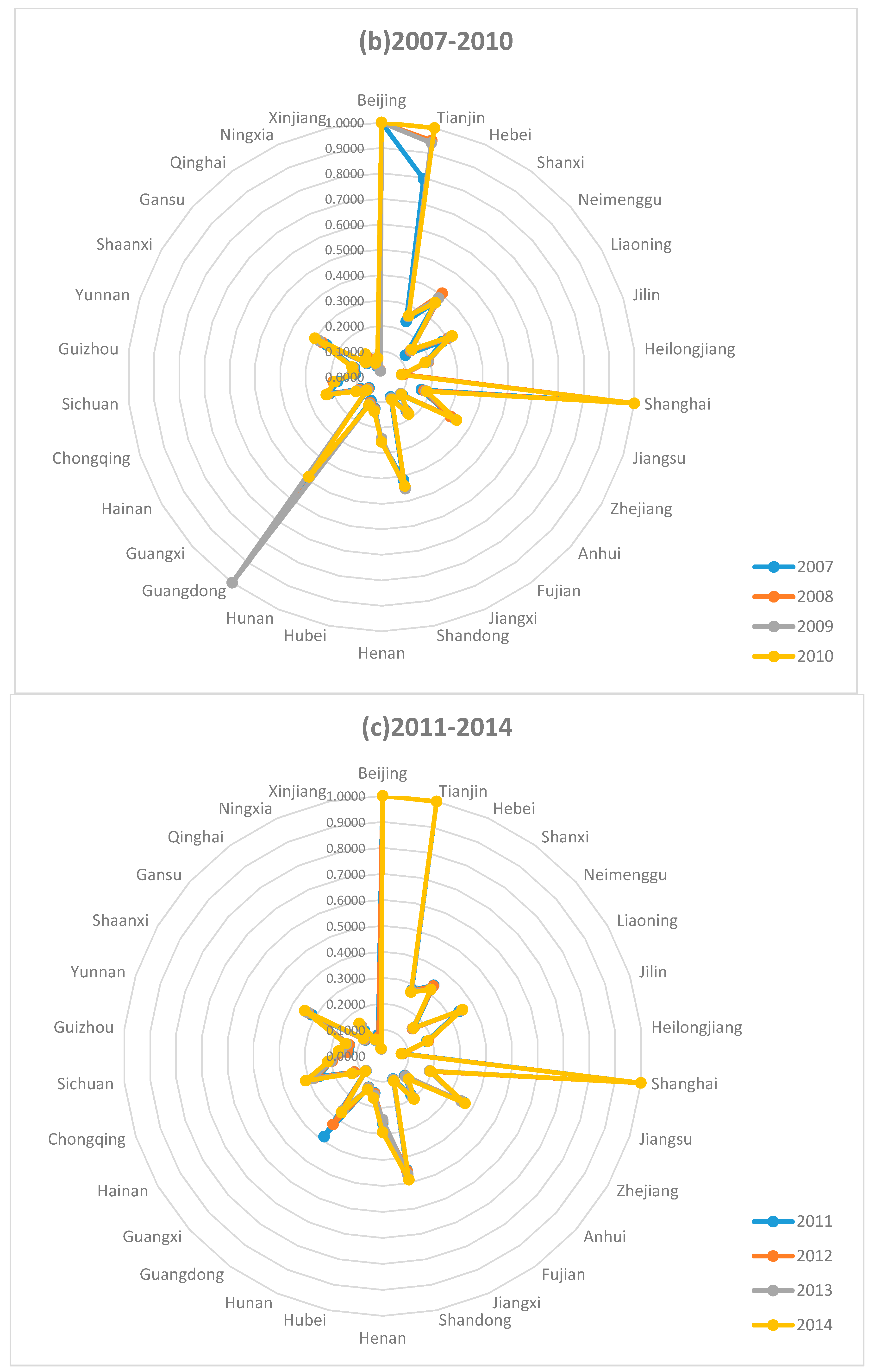
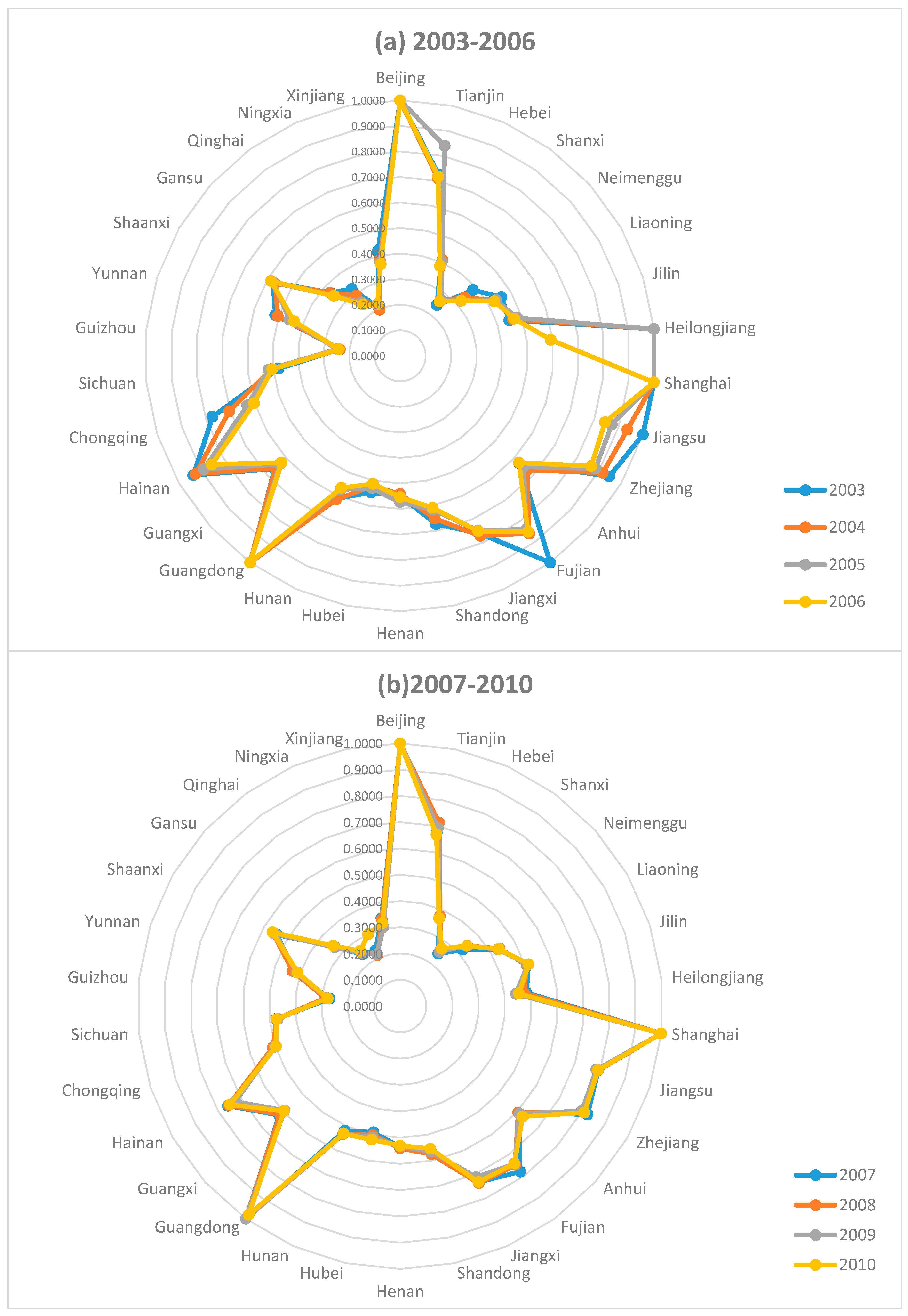
We also compare the Total Factor Efficiency of Water resource and Total Factor Efficiency of Energy between different provinces (see Figure 4 and Figure 5).

From the calculation results, we found distinct characteristics and trends of the Total Factor Efficiency of Water resource (TFEW) and the Total Factor Efficiency of Energy (TFEE) in China.

(1) Different Development Level of TFEW across the Provinces, Which Are Inconsistent with the Economic Advance Level of Each Province.

For the eastern provinces of China, except for Beijing and Shanghai, which have kept an optimal water resource Total Factor Input Efficiency throughout the study period, and Tianjin, which has quickly returned to the optimal water efficiency level after some fluctuations from 2006 to 2009, all other provinces have shown an unsatisfying TFEW. Major economic provinces including Guangdong, Jiangsu and Zhejiang Provinces all have a low TFEW. Except in 2003, Jiangsu Province’s TFEW has never achieved above 0.2 throughout the study period. Since 2004, Fujian Province has experienced a sharp decrease in TFEW, as is the case with Guangdong Province since 2010. The TFEW of these two provinces in 2014 were only 20.56% and 26.93%, respectively, of their highest TFEW level throughout the study period. The main reason is that, along with the fast economic development of eastern regions, the wastewater emissions by these provinces have also been increasing. As two of the top-ranking provinces in China in terms of total regional GDP of 2014, Guangdong Province had a wastewater emission of 9.05 billion tons in that year, while Jiangsu Province had a wastewater emission of 6.01 billion tons. The total wastewater emission of these two provinces combined has already exceeded the total wastewater emission of 11 western provinces in China combined in that same year (14.52 billion tons). Although the pressure of water resources faced by the eastern provinces is reducing, the per capita water withdrawals falls from 444.68 cubic meters per person in 2004 to 381.62 cubic meters per person in 2014 [1], the raise of TFEW in major economic provinces will help to further reduce the pressure and create greater room for future development.

The TFEW in northeast China is also far from optimal. The TFEW of Liaoning Province has declined from its highest level 1 in 2003 to 0.2763 in 2007. Although its water efficiency has improved a little in recent years, in 2014, it has only climbed to 35.49% of the highest level. The TFEW of Jilin Province has also experienced sharp decrease. In 2014, it was only 35.30% of its highest level during the study period (0.5167 in 2003). The decline of TFEW in Heilongjiang Province is even more shocking. After its prime level of 1 from 2003 to 2005, its water efficiency has kept declining to 0.0726 in 2014, which was only 7.26% of its highest level. There is no province in China other than Heilongjiang that has witnessed such a sharp and rapid decline in TFEW. We have noticed that the development trend of TFEW in northeast China has accompanied the trend of fast-growing emissions of wastewater and slowing-down GDP growth of the provinces mentioned above. Take Heilongjiang Province as an example, its wastewater emission of 2011 has increased by 27.06% compared with that of 2010. At the same time, its GDP growth rate has been declining since 2010. Its GDP growth rate in 2014 was only 4.04%. Meanwhile, the per capita water consumption in the northeast provinces increased from 451.55 cubic meters per person in 2004 to 585.31 cubic meters per person in 2014 [1]. Therefore, the northeast provinces need to maintain economic growth while increasing the TFEW. It can reverse the current decline tendency of economic growth on the basis of using existing water resources more effectively. For central regions of China, the TFEW of Shanxi, Anhui, Henan, Hubei and Hunan Provinces have all experienced continuous decline since 2003. During our study period, the per capita water consumption in the central provinces increased from 343.39 cubic meters per person in 2004 to 405.20 cubic meters per person in 2014 [1]. Although, from their development trend, we have seen some recovery in TFEW of Anhui, Hubei and Hunan Provinces in the last five years, their efficiency level was still quite far away from their highest level in 2003. Despite being the province with the smallest decline in TFEW in central China, Jiangxi Province also has some significant problems. First, its TFEW across the study period has always been low (all lower than 0.11). Second, although its TFEW has seen some recovery since 2009, its level in 2014 was still lower than its highest level in 2003. Therefore, the central provinces need to recognize the realistic and potential pressure of water resources utilization and improve the TFEW.

For western regions of China, although the per capita water consumption was essentially flat (from 669.59 cubic meters per person in 2004 to 664.18 cubic meters per person in 2014 [1]), their TFEW throughout the study period is the lowest in China. In 2014, the TFEW of Guangxi, Gansu, Ningxia, and Xinjiang Provinces were lower than 0.1, and even the highest level among western provinces of Shaanxi Province was only 0.3462. From data of the last five years, we have seen an improving trend in TFEW of Inner Mongolia, Chongqing, Sichuan, Guizhou, Shaanxi, Gansu, Qinghai, and Ningxia Provinces, with the latter seven provinces reaching their highest TFEW in 2014 and ranking top among all the four economic zones of China. The pressure of water resources is not so significant. However, because the absolute level of TFEW is still quite low, there are still many improvements to work on in the future.

In conclusion, the TFEW across different provinces in China are generally quite low, with unsatisfying development trend in recent years. Except for cities such as Beijing (including Tianjin) and Shanghai which have kept an optimal TFEW level across the study period, all the other provinces still have a low level, even for the economically developed regions in the east. Our calculation result has also proved that if China still makes GDP growth as its most important and even the only indicator for measuring economic development, the huge amounts of undesirable output (such as wastewater) generated along with the fast economic growth will negatively influence the total factor efficiency of water resource in China.

(2) The TFEW Generally Lower Than TFEE

Except for Beijing and Shanghai, the TFEW is clearly lower than TFEE across different provinces in China. Even for the eastern regions with the most developed economy, this case still widely exists. Take Guangdong, the province with the highest GDP level in China, as an example, except for the years from 2003 to 2009 with optimal efficiency level, from 2010 to 2014, the TFEW is even lower than 50% of the TFEE. The proportion of TFEW/TFEE has also been declining across the years, from 49.63% in 2010 to 36.70% in 2014. Another major developed province in eastern China, Jiangsu is also facing the same situation, only with an even shocking contrast between the TFEW and TFEE. During the entire study period, the ratio between TFEW against TFEE has never reached above 30%. In 2004 and 2006, this ratio was even lower than 20%. This trend did not stop until 2013, and the above ratio has gradually recovered to 27.4% and 27.7%, respectively, in 2013 and 2014. Evidence above has shown that for these two provinces, the energy resource input has played a more important role in GDP growth than the water resource. This has also shown that for coastal regions such as Guangdong and Jiangsu Province whose water resource is much richer than central and western regions of China, the ratio between TFEW against TFEE is clearly lower than the other regions due to less attention on the utilization efficiency of water resource and emission of wastewater.

Among the eastern provinces, Tianjin is one of the very few cities in China with higher TFEW compared with TFEE. Moreover, with the optimal or close-to-optimal level of TFEW, Tianjin’s TFEE has kept an upwards trend. Since 2011, Tianjin has reached the optimal level of 1 for both TFEW and TFEE. With its neighboring city, Beijing, keeping an optimal level of TFEW and TFEE and the development of economic integration covering Beijing, Tianjin and Hebei by the Chinese government, it is not surprising for Tianjin to achieve such outstanding efficiency. In 2004, the department with the most authority in economic administration within the Chinese government, the National Development and Reform Commission, organized a series of meetings for the Heads of Beijing, Tianjin and Hebei to reach the so-called “Langfang Consensus” regarding the fundamental topics in the economic integration of these three regions. In addition to the regular discussion and negotiation system between the Development and Reform Commissions of these three cities, as well as regular joint conference arrangements between the senior leaders, they have also decided to coordinate major topics of ecosystem construction and environmental protection within this region, and jointly initiate measures on water resource protection and optimal utilization [37]. Thanks to their unique geographic location and administrative status as municipality directly under the central government, Tianjin and Beijing have always been working closely together on economic development, resource utilization and environmental protection, with closer cooperation and faster integration compared with that of Hebei. Later on, in the “Eleventh Five-Year Plan” of China published in 2006, the economic integration and regional development of Beijing, Tianjin and Hebei as a whole has also been mentioned. After that, the National Development and Reform Commission officially initiated the plan for a “Beijing-Tianjin-Hebei Metropolitan Area” [38]. In February 2014, Chinese President Xi Jinping has even raised the topic of integrated development of Beijing-Tianjin-Hebei area to the level of “major national strategy” [39]. Therefore, from the perspective of TFEW, Tianjin has become the biggest winner through this “Beijing-Tianjin-Hebei Integration Initiative”.

For northeast regions of China, the structure of TFEW compared with TFEE also shows a similar pattern with that of the eastern region. For example, the ratio between TFEW against TFEE of Liaoning, Jilin and Heilongjiang Provinces within the study period has shown a clear declining trend, especially for Jilin and Heilongjiang Provinces. For Heilongjiang Province, although its TFEW and TFEE have reached the optimal efficiency level of 1 from 2003 to 2005, both indicators have experienced a sharp decline in the following years. In 2014, the ratio between TFEW and TFEE was merely 18.02%, which also accompanied the slowing-down trend of Heilongjiang Province’s GDP growth as mentioned above. The only highlight in the northeast region is Liaoning Province. Although since 2003 its optimal level of TFEW has seen a clear drop, the ratio between TFEW against TFEE has seen an upwards trend since 2008, which reached its highest level of 84.40% across the study period in 2014.

For central regions, except Shanxi Province, the TFEW is also lower than TFEE. Take Jiangxi Province with the lowest ratio of TFEW versus TFEE as an example, this ratio has always been around 15%, and has only reached slightly above 15% in 2013, which further climbed to 17.05% in 2014. This ratio of Anhui, Hubei and Hunan Provinces has also been lingering around 30% during the study period. In comparison, this ratio of Shanxi Province has always been among the highest in China. Although this ratio has slightly declined during the study period, Shanxi Province’s ratio between TFEW and TFEE has reached 152.77% in 2014, which ranked first nationwide and was only followed by Tianjin. However, we must also recognize the fact that this top-ranking ratio is mainly due to the low TFEE of Shanxi Province. In 2014, the TFEE of Shanxi was only 0.2058, which was among the lowest in China and only higher than three provinces: Xinjiang (0.1990), Qinghai (0.1848) and Ningxia (0.1782). Therefore, in addition to keeping a high TFEW, more importantly, Shanxi needs to improve its TFEE as soon as possible.

For western provinces, the ratio of TFEW against TFEE is generally quite low, and the absolute level of TFEW and TFEE are both quite low. For certain provinces such as Gansu, Ningxia, and Xinjiang, the TFEW has never been above 0.1 across the study period, representing the lowest level in China. Evidence above shows that the TFEW as well as TFEE of the western provinces in China still have a large improvement area in the future: continuously improve the TFEW and TFEE along with fast economic development.

5. Conclusions

This paper has conducted both theoretical and empirical analyses on the Total Factor Efficiency of Water resource (TFEW) and Energy resource (TFEE) of China from 2003 to 2014. We put wastewater as undesirable output on the output side of the DEA Model rather than on the input side as most traditional studies did. We have also designed our own MATLAB programming based on the DEA Model.

Based on the above analysis, we have reached the following conclusions. With increasing input and investment of water resource and energy resource, China has enjoyed a fast economic development. However, despite this fast GDP growth, the Total Factor Efficiency of such production process is still far from optimal. Except for a few highly-developed cities such as Beijing and Shanghai, for most provinces in China (even those with top ranking GDP output in the eastern region of China, such as Guangdong and Jiangsu Provinces), their TFEW still requires huge improvements. Moreover, because the TFEW and TFEE are both quite low in the northeast, central and western regions of China (see Shanxi Province as a typical example), there is still a long way to go for China to optimally utilize water resource and significantly improve the TFEW and TFEE.

Based on the findings, we have provided policy recommendations to improve water efficiency.

(1)

Change the goal setting for economic development and reform the mechanism of government official assessment and promotion. Since the reform and opening-up of China, GDP growth has always been the most important measurement of economic development as well as determinant for official promotion in different provinces. However, under the background of huge amounts of undesirable output and low TFEW, China need to include TFEW into the performance assessment system of government departments and put enough emphasis on it. In order to encourage and motivate different provinces to work on water efficiency improvement, we must change the past government assessment system as well as economic development model solely pursuing GDP growth.

(2)

Continuously improve the legal system governing water resources, enhance monitor on water consumption as well as promotions on water conservation, and awaken our people’s awareness on water saving. China must construct and maintain a healthy legal system to encourage water saving and pollution reduction. We must also strengthen the target and accountability on water saving and implement related rewards and punishment measures, which should exist through all the stages including investment, construction, production and consumption. The purpose is to construct a green input–output model with efficient water resource usage and reduced wastewater emission.

(3)

Develop new and advanced technologies on efficient utilization and recycling of water resources to facilitate the strategic transition towards water saving by technological means. By greatly developing new technologies and inventions on better utilization of water resource, we can maximize the water efficiency and minimize wastewater emission. At the same time, we must try our best to continuously improve the scale economies of water resource and the TFEW to achieve the optimal water efficiency on both the input and the output sides.

(4)

Facilitate and strengthen inter-provincial and international cooperation and exchange on water resource utilization. On the one hand, within China, we should facilitate the technology transfer and equipment support from provinces with high TFEW to provinces with poor TFEW, as well as design and implement appropriate policies regarding water resource input and water saving based on each province’s geographical characteristics. On the other hand, we should introduce internationally advanced water resource utilization technology and equipment from other countries to improve our overall strength on water resource utilization across the country.