The Short-Term Power Load Forecasting Based on Sperm Whale Algorithm and Wavelet Least Square Support Vector Machine with DWT-IR for Feature Selection

Abstract

Short-term power load forecasting is an important basis for the operation of integrated energy system, and the accuracy of load forecasting directly affects the economy of system operation. To improve the forecasting accuracy, this paper proposes a load forecasting system based on wavelet least square support vector machine and sperm whale algorithm. Firstly, the methods of discrete wavelet transform and inconsistency rate model (DWT-IR) are used to select the optimal features, which aims to reduce the redundancy of input vectors. Secondly, the kernel function of least square support vector machine LSSVM is replaced by wavelet kernel function for improving the nonlinear mapping ability of LSSVM. Lastly, the parameters of W-LSSVM are optimized by sperm whale algorithm, and the short-term load forecasting method of W-LSSVM-SWA is established. Additionally, the example verification results show that the proposed model outperforms other alternative methods and has a strong effectiveness and feasibility in short-term power load forecasting.

1. Introduction

Energy and environmental issues have increasingly contributed to the transformation of human energy consumption patterns, and how to improve energy efficiency, reduce environmental pollution and achieve sustainable energy development has been the topic of today’s common interest [1]. The integrated energy system (IES), which combined the hot and cold power micro-grid, can carry on the unified dispatching of electric power, natural gas energy and distributed energy. Furthermore, the integrated energy system can not only meet a variety of load requirements, but can also improve the energy efficiency of energy system and environment benefits; it has become an important direction for future energy system development [2]. However, there still exist some problems in the actual operation of the distributed energy, such as power output randomness, weak system stability and so on [3]. Therefore, to accurately forecast the power load of IES is of great significance, which can not only help to prove the stability of the system operation, but can also promote the efficiency of various energy sources. The accuracy of short-term power load prediction directly affects the quality of the prediction work.

At present, the load forecasting methods are mainly divided into two categories: traditional forecasting method and the intelligent prediction method. Separately, the traditional prediction method mainly includes time series prediction, regression analysis, gray prediction, fuzzy prediction and so on. For example, A.E. et al. [4] proposed a multiple equation time-series model for forecasting day-ahead electricity load. Cui et al. [5] presented a combined model of HP Filter-SARIMA-Revised ARMAX optimized by regression analysis was introduced to forecast short-term power load. Zhao et al. [6] presented an improved grey model optimized by a new optimization algorithm Ant Lion Optimizer for annual power load forecasting and the rolling mechanism was introduced to improve the forecasting accuracy. Coelho et al. [7] used a novel hybrid evolutionary fuzzy model with parameter optimization for load forecasting in a MG scenario. As can be seen from the above references, this kind of forecasting method has a mature theoretical basis, and its calculation process is simpler and easier to understand; however, this kind of method is unable to deal with non-linear forecasting problem due to theoretical limitation, its application object is often relatively simple, and the prediction accuracy usually fails to meet the expectations.

With the development of modern computer technology and the continuous improvement of mathematical theory, intelligent forecasting methods are favored by many scholars for deep research. Artificial neural network (ANN) and support vector machine (SVM) are usually attractive to many scholars for solving short-term power load forecasting problems. As shown in paper [8], an artificial neural network (ANN) model with a back-propagation algorithm was presented for short-term load forecasting in micro-grid power systems. In paper [9], several univariate approaches based on neural networks were proposed and compared, which included multi-layer perceptron, radial basis function neural network, generalized regression neural network, fuzzy counter propagation neural networks, and self-organizing maps. Rana et al. [10] introduced an advanced wavelet neural networks for very short-term load forecasting, and the complex electricity load data was decomposed into different frequencies by the proposed method to separately realize the load forecasting. In paper [11], an effective short-term load forecasting model based on the generalized regression neural network with decreasing step fruit fly optimization algorithm was proposed. However, the ANN has slow convergence speed and easy to fall into the local optimal problem, which leads to the decrease of the prediction accuracy.

Since the SVM model can avoid the local optimum problem, it has been widely used in the research field of load forecasting. For example, Pan et al. [12] and Ceperic et al. [13] used the SVM model to verify its effectiveness and feasibility in power load forecasting. To improve the prediction performance, some scholars attempt to use the evolutionary algorithms to determine the parameters values of SVM. Pai et al. [14] firstly proposed to use the genetic algorithms (GA) to determine the parameters of SVM in solving the load forecasting problems. Ren et al. [15] used particle swarm optimization (PSO) to optimize the parameters of the SVM model for power load forecasting to improve the prediction accuracy. Zhang et al. [16] proposed a novel model for electric load forecasting by the combination of singular spectrum analysis, support vector machine and Cuckoo search algorithms. Compared with the neural network, SVM model is used to obtain a better result for load forecasting, but the speed of SVM algorithm is still not fast enough. The choice of kernel function has great influence on the running results, and the choice of kernel function parameters depends on the experience value.

Thus, some scholars try faster LSSVM for load forecasting. Li et al. [17] proposed a LSSVM-based annual electric load forecasting model that used Fruit Fly Optimization Algorithm (FOA) to automatically determine the appropriate values of the two parameters for the LSSVM model. Niu et al. [18] introduced a wavelet least square support vector machine model optimized by the improved fruit fly optimization algorithm. Sun et al. [19] presented a least-squares support vector machine method based on improved imperialist competitive algorithm through differential evolution algorithm so as to improve the accuracy of short-term load forecasting. To improve the accuracy of load forecasting, Liang et al. [20] presented a hybrid model based on wavelet transform and least squares support vector machine, which was optimized by an improved cuckoo search. Through the above analysis, we can find that some researchers usually apply optimization algorithms to optimize the parameters of LSSVM, so as to solve the blind selection problems of the penalty coefficient and kernel parameters. There are various optimization algorithms that used to optimize the parameters of SVM in terms of overcoming local optimal problem, such as particle swarm optimization algorithm (PSO) [21], genetic algorithm (GA) [14,22], artificial bee colony algorithm (ABC) [23], fruit fly optimization algorithm (FOA) [17,18,23], ant colony optimization algorithm (ACO) [24], imperialist competitive algorithm (ICA) [19], cuckoo search algorithm (CS) [20], etc.

Although the above optimization algorithms have their own advantages, each of them also emerges some corresponding shortcomings. For example, FOA cannot guarantee the convergence to the best solution, and can easily fall into the local optimum, which leads to a decrease in prediction accuracy. Imperialist competitive algorithm will show premature convergence in different situations. Cuckoo search has low searching efficiency and long calculation time, and its local search accuracy is not high, and it cannot fully meet the needs of the LSSVM parameter optimization problem. Actually, these optimization algorithms always use the best sections to achieve the global optimum and abandon bad ones. Due to this kind of optimization mechanism, they do not make the utmost usage of the data information and the obtained LSSVM parameters cannot reach the expected forecasting accuracy. Therefore, this paper tries to adopt the sperm whale algorithm (SWA) to optimize LSSVM parameters.

The sperm whale algorithm (SWA), first proposed by Ebrahimi and Khamehchi in 2016, is a brand new swarm intelligent optimization algorithm, which is mainly to simulate the whale’s life style [25]. One of the great advantages of SWA over others is that it simultaneously uses the best and the worst answers to obtain the global optimal values. The sperm whale algorithm can avoid premature convergence and prevent it from falling into local optimal by creating different subgroups. Furthermore, the step that the worst results through search space center reflection transferring to expected space, greatly reduces the computing time of the algorithm, and also improves the search efficiency of the algorithm. Currently, the sperm whale optimization algorithm has less application in other areas. Therefore, it may be a good alternative to use it to optimize the LSSVM parameters based on its unique searching characteristics. In addition, the feature selection is also important when faced with the problem of obtaining more useful influential factors and dealing with a large amount of data in load forecasting task. The term of feature selection is to identify and select the suitable input vectors for regression model to reduce the redundancy and improve the computational efficiency. Thus, this paper intends to use the discrete wavelet transform (DWT) and inconsistency rate (IR) model to make the feature selection.

The main structure of this article is as follows. In Section 2, the mathematical formulation of W-LSSVM is presented. The sperm whale algorithm is introduced in Section 3. The feature selection based on discrete wavelet transform and inconsistency rate is presented in Section 4. In Section 5, the parameters are given by W-LSSVM-SWA in example verification, and numerical testing results and comparisons are stated in detail. Finally, some conclusions are proposed in Section 6.

2. Wavelet Least Square Support Vector Machine

LSSVM is an extension of the standard support vector machine (SVM), nonlinearly mapping the input into a high-dimensional feature space to construct optimal decision surface [26]. Following the principle of risk minimization, LSSVM transforms the inequality constraints of SVM into solving equations, which simplifies the computational complexity and increases the speed of operation [27].

It is supposed that there are N samples set as $T={\left\{\left(x_i,y_i\right)\right\}}_{i=1}^N$, the regression model can be indicated as follows:

$$y\left(x\right)={\mathit{w}}^T•\varphi \left(x\right)+b$$

(1)

where $\varphi (\ast )$ is the mapping function; $\mathit{w}$ represents the weight vector; and $b$ is the bias. In LSSVM, the optimization can be described as the following function:

$$min\frac{1}{2}{\mathit{w}}^T\mathit{w}+\frac{1}{2}\gamma {\displaystyle \sum _{i=1}^N{\mathit{\xi }}_i^2}$$

(2)

$$s\cdot t y_i={\mathit{w}}^T\varphi \left(x_i\right)+b+{\mathit{\xi }}_i,i=1,2,3,\cdots N;$$

(3)

where the penalty factor $\gamma$ is used for the balance between model’s complexity and accuracy; and ${\xi }_i$ serves as error. To address the above equations, the Lagrange function is defined as below:

$$L\left(\mathit{w},b,{\mathit{\xi }}_i,{\alpha }_i\right)=\frac{1}{2}{\mathit{w}}^T\mathit{w}+\frac{1}{2}\gamma {\displaystyle \sum _{i=1}^N{{\mu }_i\mathit{\xi }}_i^2}-{\displaystyle \sum _{i=1}^N{\alpha }_i}\left[{\mathit{w}}^T\varphi \left(x_i\right)+b+{\mathit{\xi }}_i-y_i\right]$$

(4)

where ${\alpha }_i$ is the Lagrange multiplier. Partial derivatives of $\mathit{w}$, $b$, ${\xi }_i$, and ${\alpha }_i$ are taken, equaling to zero, in Equation (5).

$$\{\begin{array}{l}\frac{\partial L}{\partial \mathit{w}}=0\to \mathit{w}={\displaystyle \sum _{i=1}^N{\alpha }_i\varphi \left(x_i\right)}\\ \frac{\partial L}{\partial b}=0\to {\displaystyle \sum _{i=1}^N{\alpha }_i=0}\\ \frac{\partial L}{\partial \xi }=0\to {\alpha }_i=\gamma {\mu }_i{\xi }_i\\ \frac{\partial L}{\partial \alpha }=0\to {\mathit{w}}^T+b+{\xi }_i-y_i=0\end{array}$$

(5)

Then, the optimization problem is changed into Equation (6) by eliminating $\mathit{w}$ and ${\mathit{\xi }}_i$.

$$\left[\begin{array}{cc}0& {\mathit{e}}_n^T\\ {\mathit{e}}_n& \mathit{\Omega }+{\gamma }^{-1}{\mu }^{-1}\cdot I\end{array}\right]\cdot \left[\begin{array}{c}b\\ a\end{array}\right]=\left[\begin{array}{c}0\\ y\end{array}\right]$$

(6)

where $\mathit{\Omega }={\varphi }^T\left(x_i\right)\varphi \left(x_i\right)$; ${\mathit{e}}_n$ is an n-dimensional column, and $\alpha$ and $y$ are equal to $\left[{\alpha }_1,{\alpha }_2,...,{\alpha }_n\right]$ and ${\mathbf{\left[}{y}_1,y_2,...,y_n\mathbf{\right]}}^T$, respectively. According to Equation (6), $y\left(x\right)$ is obtained as follows:

$$y\left(x\right)={\displaystyle \sum _{i=1}^N{\alpha }_{i}K\left({\mathit{x}}_{\mathit{i}},\mathit{x}\right)}+b$$

(7)

where $K\left({\mathit{x}}_i,\mathit{x}\right)$ is the kernel function. In the present study, Gaussian kernel function in LSSVM is superseded by wavelet kernel function $K({\mathit{x}}_{\mathit{i}},\mathit{x})={\displaystyle \mathbf{\prod }_{i=1}^N\psi (\frac{x_i-x_i^{\prime }}{{\sigma }_i})}$, which will be detailed established in the next section. Hence, Equation (7) is switched by the following:

$$y\left(x\right)={\displaystyle \mathbf{\sum }_{i=1}^N{\alpha }_i{\displaystyle \prod _{i=1}^N\psi (\frac{x_i-x_i^{\prime }}{{\sigma }_i})}}+b$$

(8)

$$\psi (x)=\cos (1.75x)\cdot \exp (\frac{-x^2}{2})$$

(9)

Eventually, weighted LSSVM can be acquired, as indicated in Equation (10).

$$y\left(x\right)={\displaystyle \sum _{i=1}^N{\alpha }_i{\displaystyle \prod _{i=1}^N\{\cos [\frac{1.75(x_i-x_i^{\prime })}{{\sigma }_i}]\cdot \exp [\frac{-{(x_i-x_i^{\prime })}^2}{2}]\}}}+b$$

(10)

The use of wavelet kernel function instead of traditional radial basis function is mainly based on the following reasons [28]:

(a)

Wavelet kernel function has an advantage in stepwise data-description and is superior to Gaussian kernel function when applied in LSSVM to simulate arbitrary functions accurately.

(b)

Compared with Gaussian kernel function, wavelet kernel function is orthogonal or nearly orthogonal rather than relevant or even redundant.

(c)

Particularly because of multi-resolution analysis and processing of the wavelet signal, wavelet kernel function has strong capability in nonlinear processing, which immensely promotes LSSVM’s generalization ability and robustness.

3. Sperm Whale Algorithm

Deriving from the life style of sperm whales, a new efficient multi-objective optimization algorithm called sperm whale algorithm (SWA) [25] is mathematically modeled. In SWA, each answer denotes a sperm whale. By virtue of multiple populations’ common search, $m\times n$ number of individuals should be created as the initial population. Subsequently, the primary population is divided into $n$ Temporary Sub-group (TSG), each containing $m$ members. As shown in Figure 1, a new Main Sub-group (MSG) embodying $n$ members is produced through a randomly selected TSG until $m$ MSGs are generated for iterative optimization. The construction of various sub-groups is aiming at preventing SWA from terminating prematurely and falling into local optimum. In this algorithm, MSG is created for the following operations:

(1)

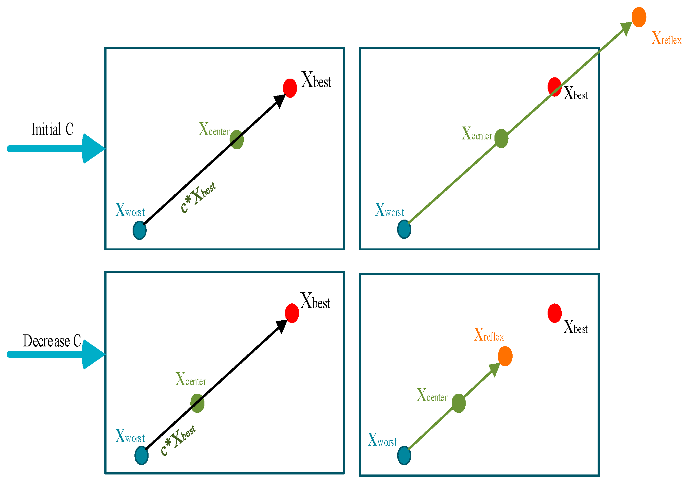
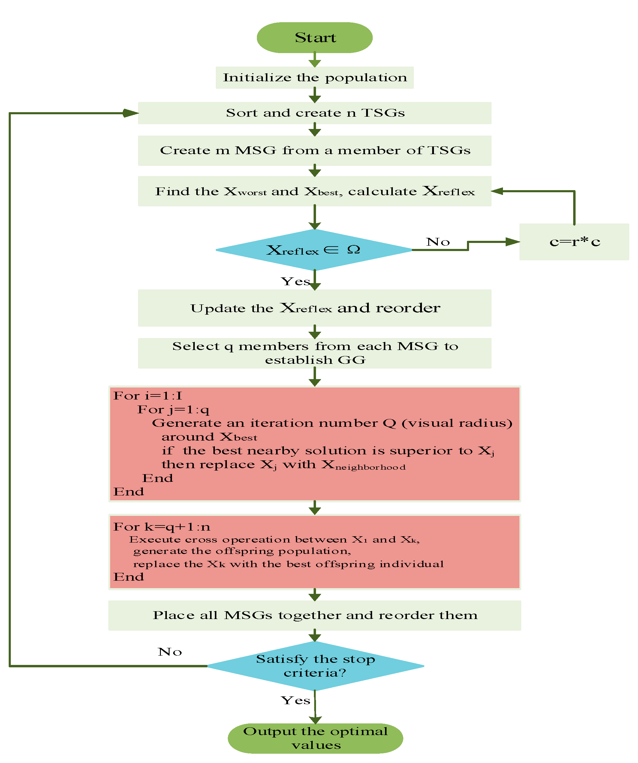
Each sperm whale undergoes two locations in breathing–feeding cycle (it breathes on the sea but takes food undersea), so that the objective function will be calculated by both two positions (current position and relative position). Nevertheless, the best answer of the relative position does not make contributions to seeking the global optimal answer and even increases the computing time, which is the reason for only reflecting the worst answer. In light of these, taking the information exchange between whales into account, location of the worst answer can be transferred into desired space by the reflection to the center of the search space. Thus, as illustrated in Figure 2, the worst and best answers are on the spatial line connecting worst answer and its reflection. Assume that the worst and best whales are named as $X_{worst}$ and $X_{best}$, respectively, so:

$$X_{center}=X_{worst}+C\times X_{best}$$

(11)

$$X_{reflex}=X_{worst}+2\times (X_{center}-X_{worst})=2X_{center}-X_{worst}$$

(12)

where $X_{center}$ is conceived as the reflection center and $C$ refers to center factor. Besides, $X_{reflex}$ is the result obtained from $X_{worst}$ to $X_{center}$.

In addition, if $X_{reflex}$ is located outside the search space, $c$ should diminish in accordance with $c=r\times c_i$, in which $c_i$ is the initial central factor and $r$ called the shrinkage factor is less than 1. In the global optimization problem, it is within the scope of the research space to select the parameter $c$. Furthermore, $C$ is presumed as a $1\times n$ vector and $n$ is the number of decision variables. Then,

$$fori=1:n$$

$$X_{\min }(i)\le X_{reflex}(i)\le X_{\max }(i)$$

(13)

$$\underset{Equation(2)}{\to }{X}_{\min }(i)\le 2X_{center(i)}-X_{worst}(i)\le X_{\max }(i)$$

(14)

$$\underset{Equation(1)}{\to }{X}_{\min }(i)\le 2\times (X_{worst}(i)+C(i)\times X_{best}(i))-X_{worst}(i)\le X_{\max }(i)$$

(15)

$$\to X_{\min }(i)\le X_{worst}(i)+2C(i)\times X_{best}(i)\le X_{\max }(i)$$

(16)

$$\to \frac{X_{\min }(i)-X_{worst}(i)}{2X_{best}(i)}\le C(i)\le \frac{X_{\max }(i)-X_{worst}(i)}{2X_{best}(i)}$$

(17)

$$c=rand\times Min(C)$$

(18)

There is no need to check whether $X_{reflex}$ is beyond the search space. Consequently, not only does this program speed up the operation to a certain extent, but it also reduces the number of parameters and dimensions. Moreover, it is unnecessary to set $r$ and $c$ specifically.

(2)

In view of sperm whales’ limited vision, a local search is carried out around the members of the Good Gang (GG) which consists of $q$ whales selected from each MSG. The search method is: members of GG can be constantly changed by iterations within the realm of definable vision Q (radius), and once a better answer is gained, the original one in GG will be replaced.

(3)

Considering the mating behavior of sperm whales (the strongest male whale mates with several female whales), there will be crossovers between the best answer in GG and other answers in MSG. Afterwards, a descendant answer randomly selected will take place of the mother answer. Finally, all answers in subgroup have a mutual substitute relationship and are reordered when the specified times of iteration are reached. It is not until the best answer is found that repetitions of the procedure above are stopped. Figure 3 displays the optimization flowchart of SWA.

As can be seen in the flowchart, no conditions are set for satisfying constraints of the fitness function, owing to application of the heuristic constraint disposal method in SWA. In this way, beneficial to algorithm’s handling capability is the adoption that no specific parameters are entailed to preset. Employing penalty function technique in SWA, fitness function will become the following:

$$F(\overrightarrow{x})=f(\overrightarrow{x})+{\displaystyle \sum _{i=1}^N{R}_i{\langle g_i(\overrightarrow{x})\rangle }^2}$$

(19)

where $f(\overrightarrow{x})$ is the objective function and $\langle g_i(\overrightarrow{x})\rangle$ is the constraint violation function $R_i$, penalty parameter of the ith inequality constraint, aims to convert the magnitude of constraint violation into objective function’s value. In case of incorrect setting of $N$ penalty parameters, they will get into trouble while a large number of equality are emerging, therefore, this heuristic constraint disposal method is put into use. With regard to pairwise comparison between two optimization results, these principles should abide by: (A) when two feasible solutions are mutually compared, the better is preferred; (B) when the feasible solution is compared with the unfeasible solution, then the feasible solution is selected; and (C) when two unfeasible solutions are compared with each other, the less violating constraint is chosen.

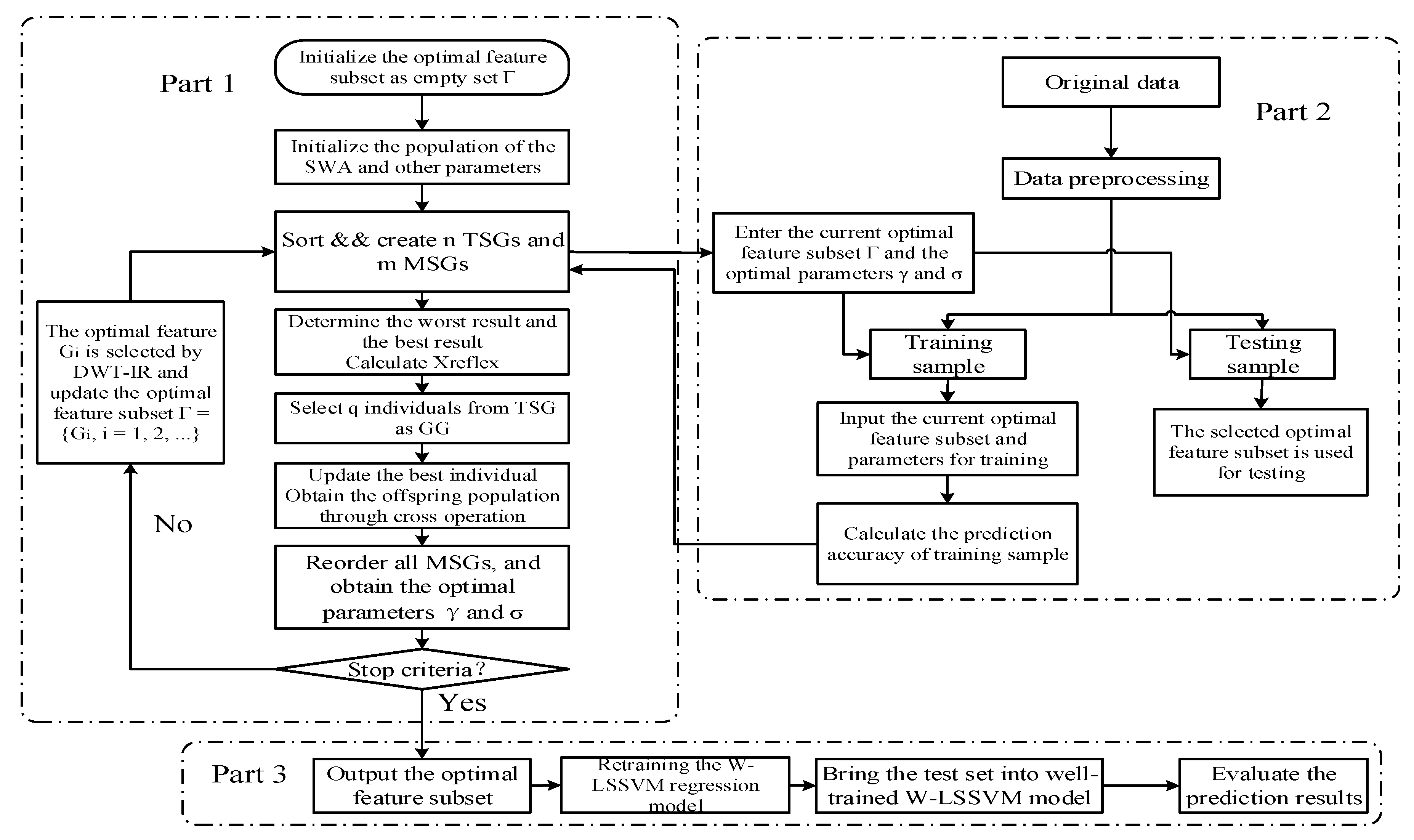
4. Feature Selection with DWT-IR

4.1. Discrete Wavelet Transform (DWT)

Discrete Wavelet Transform (DWT) has been widely used in digital signal processing, earthquake prediction, medical fault diagnosis, coding theory, quantum physics, probability theory, etc. A variety of fast Fourier transform (FFT) and discrete wavelet transform (DWT) algorithms are emerging as one of the most active fields in numerical algebra, its significance is far more than the scope of the study of the algorithm, it also opens up a new situation for the study of other science and technology [29].

Usually, continuous wavelet transform tends to have some redundancy in the data processing; to solve this problem, the discrete wavelet transform method is often used to deal with the practical problem, which also means to discrete the wavelet basis function. This kind of discrete approach is not for the time $t$, but for the stretch factor and translation factor of wavelet basis function. Typically, wavelet basis functions can be represented by the following formula [30]:

$${\Psi }_{a,t}(t)=a^{-\frac{1}{2}}\psi \left(\frac{t-\tau }{a}\right)a>0,\tau \in R$$

(20)

where $a$ represents wavelet scale stretch factor; and $\tau$ is wavelet translation factor. In general, the wavelet discretization is the discretization of parameters $a,\tau$. Let $a=2^j$ and $\tau =2^j\cdot T_s\cdot n$, the basis function of discrete wavelet can be obtained:

$${\Psi }_{j,n}(t)=2^{-\frac{j}{2}}\psi \left(\frac{t}{2^j}-n\cdot T_s\right)j,n\in N$$

(21)

The discrete wavelet coefficients for any function $f\left(t\right)$ can be defined as:

$$W{T}_f(j,n)={\displaystyle {\int }_{R}f(t)\overline{{\Psi }_{j,n}(t)}}dt$$

(22)

where $\overline{{\Psi }_{j,n}(t)}$ is the dual function of ${\Psi }_{j,n}(t)$. The discrete wavelet coefficients $W{T}_f$ can be used to construct function $f\left(t\right)$, as follows:

$$f(t)=\frac{1}{A}{\displaystyle \sum W{T}_f(j,n)\cdot {\psi }_{j,n}(t)}$$

(23)

where $A$ is a constant, and the process of DWT is shown in Figure 4.

The DWT process can be expressed as a decomposition tree composed of low frequency signals and high frequency signals [31]. In the wavelet decomposition tree, the signal decomposition process can be iterated and multi-level decomposition. To decompose the low frequency signal can get more low frequency signals, and the high frequency signal can also be decomposed to get more low frequency signals and high frequency signals. In practice, the frequency of decomposition is determined by $W{T}_f$.

In the selection of power load influence factors, a set of high frequency signals ($y_0\to y_n$) and low frequency signals ($Z_n$) can be obtained by the discrete wavelet transformation of historical data. The low frequency signal is stable and relatively smooth. In contrast, a high-frequency signal usually exhibits higher non-linear characteristics. Signal decomposition can help to analyze data features more clearly. Therefore, the input features of the model can be selected by calculating the data inconsistency rate of the different frequency signals between the data sets.

4.2. Data Inconsistency Rate (IR)

The purpose of feature selection is to distinguish the data characteristics with the strongest correlation from the load data, which makes the input vector of forecast model have a strong pertinence and low data redundancy to improve the prediction accuracy of load forecasting [32]. The data inconsistency rate can accurately describe the discrete characteristics of the input features, and different attributes can get different division patterns, different division patters can get different frequency distribution [33]. Therefore, the data inconsistency rate can be used to distinguish the classification ability of data categories. The larger the data inconsistency rate is, the worse the classification ability of the feature vector is.

Assume that a set of historical load data has $g$ features, which represented by $G_1,G_2,\cdots ,G_g$. Given that class tag $L$ has $c$ categories, and there are $n$ samples. For each sample $j$, let $X_{ji}$ represent the eigenvalues corresponding to the load feature $F_i$, then the data $j$ can be represented as $[X_j,y_j]$, $X_j=[x_{j1},x_{j2},x_{j3},\cdots ,x_{jd}]$. Continue to assume that there are $p$ feature division intervals in the load data set, denoted as $X_k^{*}(k=1,\cdots ,p)$. Therefore, the frequency of categories, obtained according to the interval division mode, is shown in

Table 1. The Class Contingency of Different Feature Patterns.

Categories	$\mathit{L}$
	1	2	$\cdots$	$\mathit{c}$
$X_1^{*}$	$f_{11}$	$f_{12}$	$\cdots$	$f_{1c}$
$X_2^{*}$	$f_{21}$	$f_{22}$	$\cdots$	$f_{2c}$
$⋮$	$⋮$	$⋮$		$⋮$
$X_p^{*}$	$f_{p1}$	$f_{p2}$	$\cdots$	$f_{pc}$

.

As shown in the Table 1, $f_{pc}$ represents the number of samples belonging to category $X_p^{*}$, thus the data inconsistency rate of the load features can be calculated as follows:

$$\tau =\frac{{\displaystyle \sum _{k=1}^p\left({\displaystyle \sum _{l=1}^c{f}_{kl}}-\underset{l}{\max }\mathbf{\left\{}{f}_{kl}\mathbf{\right\}}\right)}}{N}$$

(24)

where $f_{kl}$ is the number of data samples belonging to the $x_k$ mode. $x_k$ represents that the data set has $p$ feature division interval patterns, and $k=1,2,\cdots ,p$, $p\le N$.

The feature selection based on the data inconsistency is to select the strongest feature subset from all the features of the sample data set, and the obtained features with the smallest data inconsistency rate will maximize the characteristics of the sample dataset and reduce the redundancy caused by the repetition of the information. Assume that $Z$ is the subset of load feature set $S$, then $Z\subset S$. Let ${\tau }_z$ represent the inconsistency rate of $Z$, the feature selection is to find a subset $Z$ with minimum number of features.

If the calculated data inconsistency rate of subset $Z$ and feature set $S$ are equal, it illustrates the feature set contains many redundant features. Thus, the ideal goal of feature selection is to find a subset $Z$ that makes ${\tau }_z\approx {\tau }_S$; in other words, the feature subset $Z$ can maximize the full information of the feature set $S$, and make the data set not seem so redundant. Using the forward search method to calculate the data inconsistency rate, the calculation steps are as follows:

Step 1. Initialize the optimal feature subset is null $\mathrm{\Gamma }=\left\{\right\}$.

Step 2. Calculate the data inconsistency rate of data set $G_1,G_2,\cdots ,G_g$ which composed by each remaining feature in subset $\mathrm{\Gamma }$.

Step 3. Select the feature $G_i$ that corresponding to the minimum inconsistency rate as the optimal feature, and update the optimal feature set as $\mathrm{\Gamma }=\left\{\mathrm{\Gamma },G_i\right\}$.

Step 4. Utilize the forward search strategy to obtain the inconsistency rate statistics table of feature subsets, and arranged in ascending.

Step 5. Select a subset $\tilde{\mathrm{\Gamma }}$ with the number of selected features as small as possible, and judge whether ${\tau }_z\approx {\tau }_S$ is true; if it is true, $\tilde{\mathrm{\Gamma }}$ will be selected as the optimal feature subset.

Calculating the inconsistency rate to make the feature selection can not only eliminate redundant features but can also take into account the correlation between features. The calculation does not neglect the relationship between features, which makes the selected features can excellently represent all data information.

4.3. The Feature Selection Based on DWT-IR

The key of DWT-IR model for feature selection is to accurately calculate the inconsistency rate of different signals. Through the discrete decomposition of the feature data, the changes of the data can be directly reflected. By the calculation of the inconsistency rate, the redundancy situation can be judged intuitively, and the needed features can be effectively selected.

The calculation steps based on DWT-IR for feature selection are as follows:

Step 1. Initialize the optimal feature subset into an empty set $\mathrm{\Gamma }=\left\{\right\}$. Set the historical data to have $g$ features, denoted by $G_1,G_2,\cdots ,G_g$. Use the DWT method to constantly decompose and construct the feature data, and observe the errors between the original data and the reconstructed data until the conditions are satisfied. Thereby, obtain a set of high frequency signals $y_{ij},i=1,2,\cdots ,g,j=1,2,\cdots ,m$ and low frequency signals $Z_{in}$.

Step 2. Calculate the inconsistency rate ${\tau }_1,\cdots ,{\tau }_n$ of high frequency signal $y_{ij}$ and low frequency signal $Z_{in}$ of feature $G_i$, respectively. The final data inconsistency rate is obtained by weighted sum rules ${\tau }_{G_i}=w_1{\tau }_1+\cdots +w_n{\tau }_n$.

Step 3. Sort the data inconsistency rate ${\tau }_{G_i}$ of each feature, and select the $G_i$ with minimum inconsistent rate as optimal feature. Update the optimal feature subset $\mathrm{\Gamma }=\{\mathrm{\Gamma },G_i\}$, and judge whether ${\tau }_z\approx {\tau }_S$ is satisfied. If satisfied, output the optimal feature subset $\mathrm{\Gamma }$; if not satisfied, continue the iteration calculation.

5. Experiment and Results Analysis

5.1. Forecasting System with W-LSSVM-SWA and DWT-IR

The short-term power load forecasting method based on DWT-IR feature selection and W-LSSVM-SWA model is shown in Figure 5. As shown in the figure, the general forecasting process based on the proposed method is as follows: first, the original data is divided into training set and testing set, and the initial feature subset and initial parameters of LSSVM are put into LSSVM model to calculate the fitness function value. Second, determine the fitness function value whether to meet the conditions. If not satisfied, the DWT-IR model is used for feature selection, and the selected features are put into the LSSVM to re-calculate the fitness function value, the SWA method is adopted to optimize and control the parameters of LSSVM. It is noted that each sperm whale can be regarded as a feasible solution of the solution space, and its breathing–feeding cycle can be seen as a searching process for the parameters optimization of LSSVM. Then, the calculation cycle is repeated until the accuracy conditions are met. Finally, the optimal parameters and fitness function values are obtained.

Based on the above analysis, the proposed method in this paper mainly includes three parts. The first part is the feature selection based on DWT-IR model (Part 1), which aims to find the optimal subset and optimal parameters of the regression model through the iteration calculation. The second part is the sample training based on W-LSSVM model (Part 2); its purpose is mainly to calculate the prediction accuracy of training samples in each iteration, so the value of fitness function can be obtained. The third part is the load forecasting based on W-LSSVM model (Part 3), which aims to retrain the W-LSSVM regression model with the obtained optimal feature subset and parameters, so the test samples are accurately predicted. When the constructed feature subset does not satisfy the stop criteria, the program will continue to cycle until the expected precision is achieved.

Step 1. In addition to historical load value, this paper selects the daily maximum temperature, daily average temperature, daily minimum temperature, daily precipitation, wind speed, relative humidity, whether on weekends, and whether a holiday as the candidate features. Furthermore, this paper also selects the former $T-i$ ($i=1,\cdots ,7$) day’s maximum temperature, daily average temperature and daily minimum temperature as the main candidate features of short-term power load. All the initial candidate features are shown in

Table 2. The whole Candidate features.

$C_1,\cdots ,C_7$	$T_{t-i}^{\max },i=1,\cdots ,7$ represents the $t-i$th day’s maximum temperature
$C_8,\cdots ,C_{14}$	$T_{t-i}^{avg},i=1,\cdots 7$ represents the $t-i$th day’s average temperature
$C_{15},\cdots ,C_{21}$	$T_{t-i}^{\min },i=1,\cdots 7$ represents the $t-i$th day’s minimum temperature
$C_{22}$	$R_t$ represents the $t$th day’s precipitation
$C_{23}$	$W_t$ represents the wind speed on day $t$
$C_{24}$	$H_t$ represents the humidity on day $t$
$C_{25}$	$Cl{d}_t$ represents the cloud situation on day $t$
$C_{26}$	$M_t$ represents the month in which day $t$ is located
$C_{27}$	$Se{a}_t$ represents the season in which day $t$ is located
$C_{28}$	$Ho{l}_t$ represent whether day $t$ is holiday, 0 is holiday, 1 is not holiday.
$C_{29}$	$W{k}_t$ represent whether day $t$ is weekend, 0 is weekend, 1 is not weekend.

.

In the DWT-IR algorithm, the optimal set of features needs to be initialized as an empty set $\mathrm{\Gamma }=\left\{\right\}$. In addition, it is necessary to set the initial population number $PopNum$, TSG number $m$, MSG number $n$, initial reflection factor $c$, contraction factor $r$, GG individual number $q$, and visual radius $Q$. After the above preparation, the candidate features need to be taken into the DWT-IR model one by one to calculate the inconsistency rate of data sets $G_1,G_2,\cdots ,G_g$ in feature subsets that composed by each of remaining features of subset $\mathrm{\Gamma }$. Then, select the feature $G_i$ corresponding with minimum inconsistency rate as optimal feature, and update the optimal feature subset as $\mathrm{\Gamma }=\{\mathrm{\Gamma },G_i\}$.

Step 2. Put the feature subset of current generation into the W-LSSVM model and calculate the forecast accuracy $r(j)$ in the training process of this cycling, then the fitness value $fitness(j)$ of each cycle can be obtained. By comparing the fitness function values between each generation, the optimal feature subset can be obtained. Determine whether the stop conditions is satisfiedl if not satisfied, re-initialize the feature subset $Newsubset(i)$ and enter the new cycle until the global optimal feature subset satisfies the stop criteria. It should be noted that the parameters of W-LSSVM model also need to be initialized, and the initial value of $\gamma ,\sigma$ will be randomly assigned.

Step 3. Apply the obtained optimal feature subset into the testing sample to retrain the W-LSSVM. Furthermore, the parameters determination of W-LSSVM is the key to model training and learning ability, which directly affects the accuracy of load forecasting. Therefore, the parameters $\gamma ,\sigma$ should be optimized by SWA model rather than subjective determination.

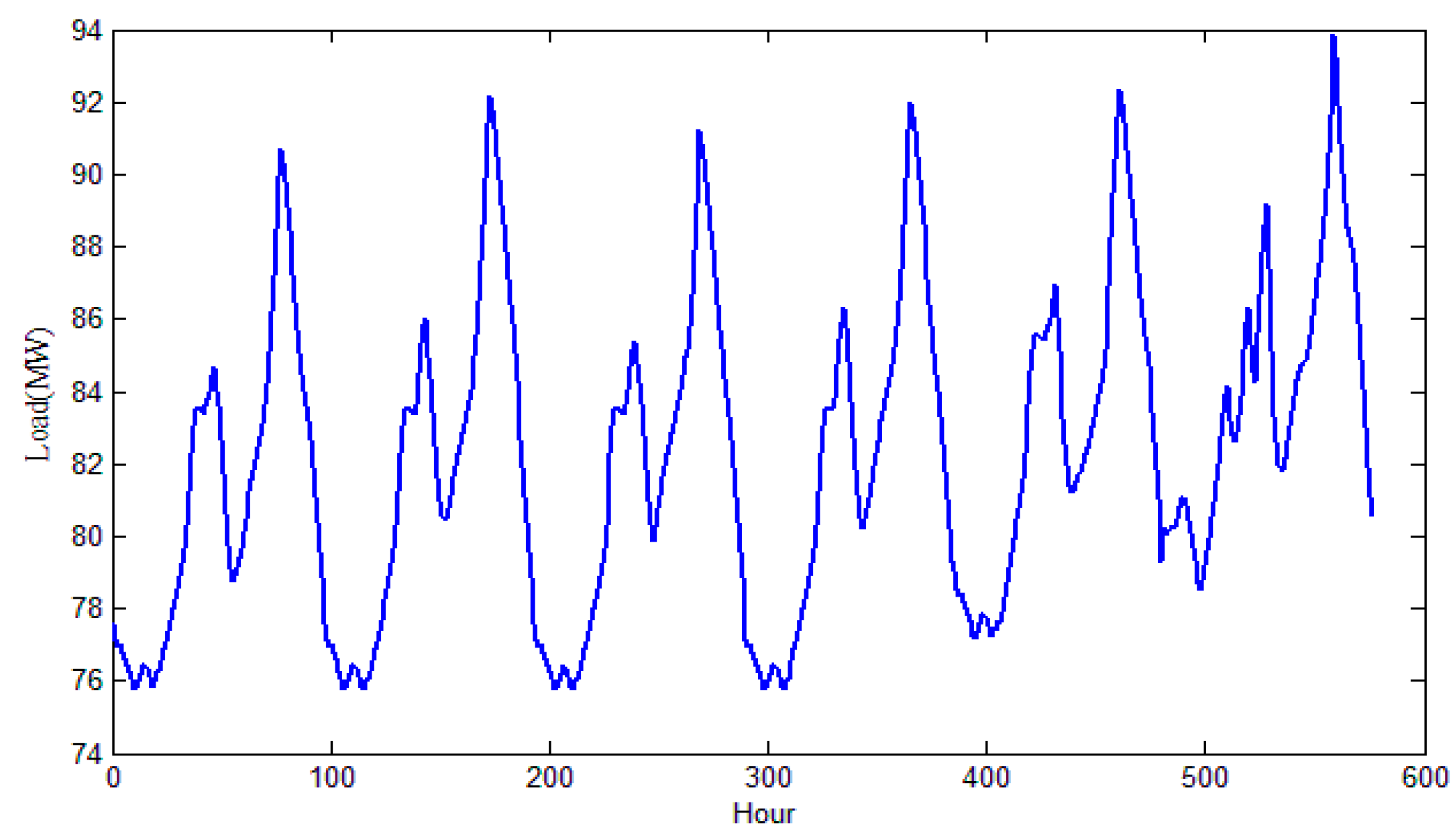
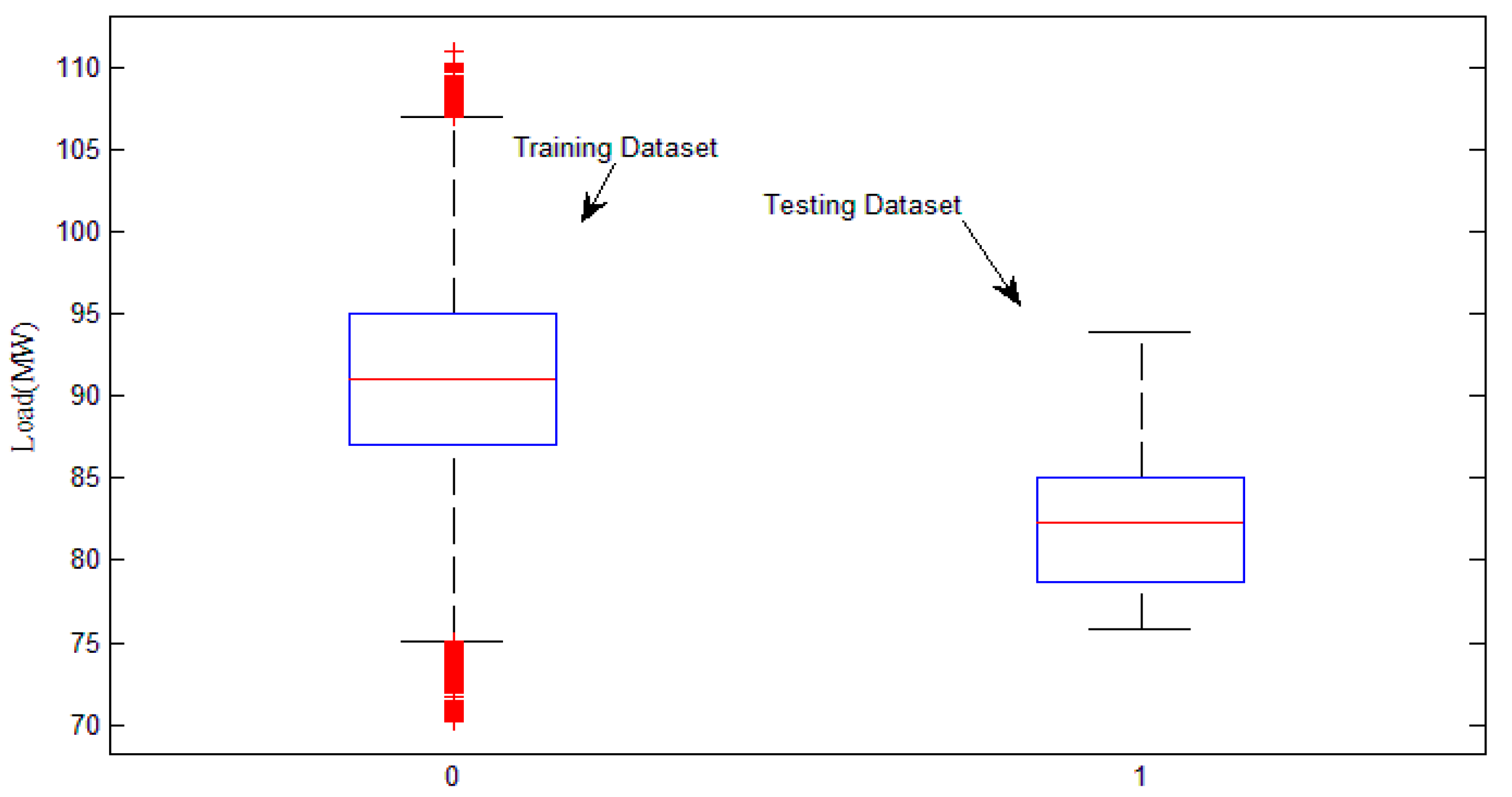
5.2. Data Selection and Pretreatment

The sample data of this paper are provided by the Sichuan Energy Internet Research Center. The power load data from 0:00 on 21 March 2015 to 10:00 on 24 April 2016 are selected as training sample and used to established the single variable time series. The power load data from 11:00 on 24 April 2016 to 24:00 on 30 April 2016 are used as testing sample. Figure 6 and Figure 7 are the distribution of training dataset and testing dataset, respectively. Figure 8 is a box-plot comparison of the training dataset and testing dataset. It can be seen in Figure 8 that the data type of the testing set is similar to that of the training set, and neither of them has an abnormal load value. In addition, the curves of training and testing dataset are relatively smooth, only their mean values and distribution are different.

For the better training and learning of the proposed model, all the historical data should be normalized in the [0, 1] interval, and the normalized formula is as follows:

$$Y=\{y_i\}=\frac{x_i-x_{\min }}{x_{\max }-x_{\min }}i=1,2,\cdots ,n$$

(25)

where $x_{\max }$ and $x_{\min }$ are the maximum and minimum load value of sample data, respectively. $x_i$ is the $i$th load point value. $y_i$ represents the value of the adjusted $i$th load point.

In this paper, the maximum and minimum relative error (Max/Min RE), mean absolute percentage error (MAPE), and root mean square error (RMSE) are used to evaluate the load forecasting results, each evaluation indexes is as follows:

$$\mathrm{Max}/\mathrm{Min}\mathrm{RE}=\mathrm{Max}/\mathrm{Min}\{\left|\frac{y_i-y_i^{\prime }}{y_i}\right|\times 100\%\}$$

(26)

$$\mathrm{M}\mathrm{A}\mathrm{P}\mathrm{E}=\frac{1}{n}{\displaystyle \sum _{i-1}^n\left|\raisebox{1ex}{$(y_i-y_i^{\prime })$}\!\left/ \!\raisebox{-1ex}{$y_i$}\right.\right|}\times 100\%$$

(27)

$$RMSE=\sqrt{\frac{1}{n}{\displaystyle \sum _{i=1}^n{(\frac{y_i-y^{\prime }}{y_i})}^2}}$$

(28)

where $y_i$ is the actual value of power load, $y_i^{\prime }$ is the prediction value of power load, and $i=1,2,\cdots ,n$.

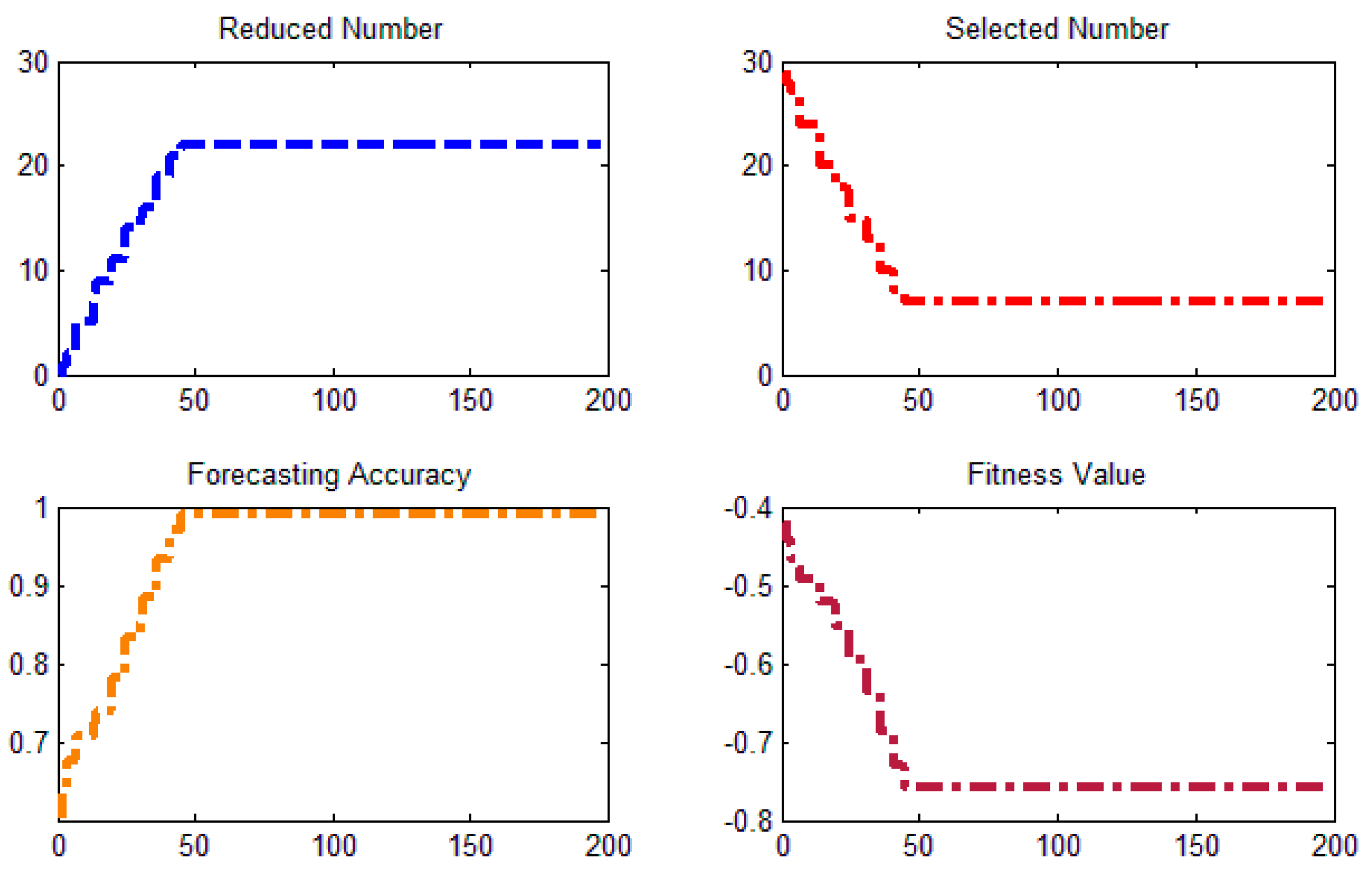
5.3. DWT-IR for Feature Selection

This part is mainly the optimal feature subset selection based on the DWT-IR model. The main purpose of feature selection is to find the optimal subset to describe the accuracy of prediction system from a specific problem, to avoid the redundant information caused by too much input vectors, resulting in lower prediction accuracy, etc. Therefore, in the short-term load forecasting system, choosing the appropriate fitness function is of great help to determining the optimal feature subset. In this paper, the fitness function based on the double factors of prediction accuracy and feature selection number is established, as follows:

$$fitness\left(x_i\right)=-(a\ast r\left(x_i\right)+b\ast \frac{1}{Numfeature(x_i)})$$

(29)

where $r\left(x_i\right)$ represents the short-term load forecasting accuracy of each iteration; $Numfeature(x_i)$ is the number of optimal features selected at each iteration; and $a,b$ are the constant between [0, 1]. From this formula, it can be inferred that the higher the prediction accuracy is and the less the number of features are, the higher the fitness function value is.

Figure 9 is the iterative process graph of discrete wavelet inconsistency rate model for training sample feature extraction.

As shown in Figure 9, the fitness curve describes the obtained fitness values in each iteration. The forecasting accuracy curve describes the prediction accuracy of the W-LSSVM model for the training sample in different iterations. The reduced number is the number of eliminated features in the convergence process. The selected number represents the number of optimal features that calculated by the DWT-IR model in the convergence process. As can be seen in Figure 9, the algorithm achieves convergence when the iteration number is 47, and the optimal fitness value is calculated to be −0.76. Moreover, the forecasting accuracy of the training sample is 98.9% at the 47th iteration, which indicates that the fitting ability of W-LSSVM is strengthened by the learning and training of algorithm, so that the prediction accuracy of the training sample reaches the highest. In addition, the number of selected features tends to be stable when the algorithm runs to the 47th, and it can be seen that the algorithm eliminated 22 redundant features from 29 candidate features.

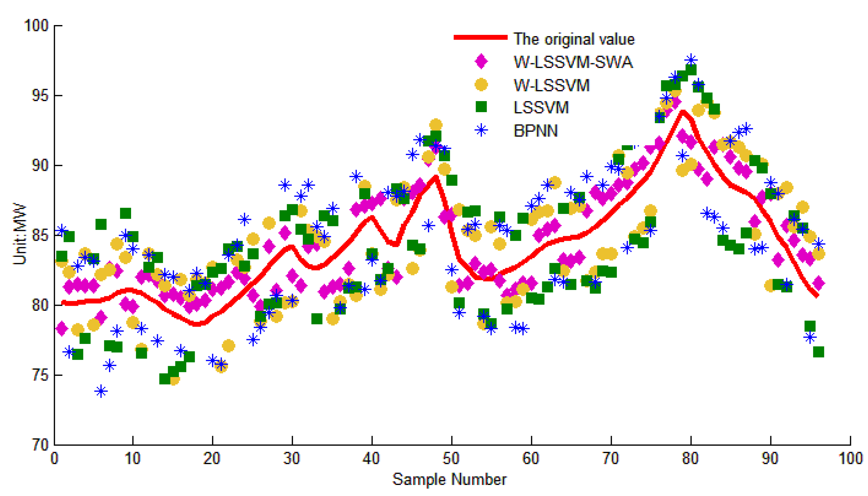
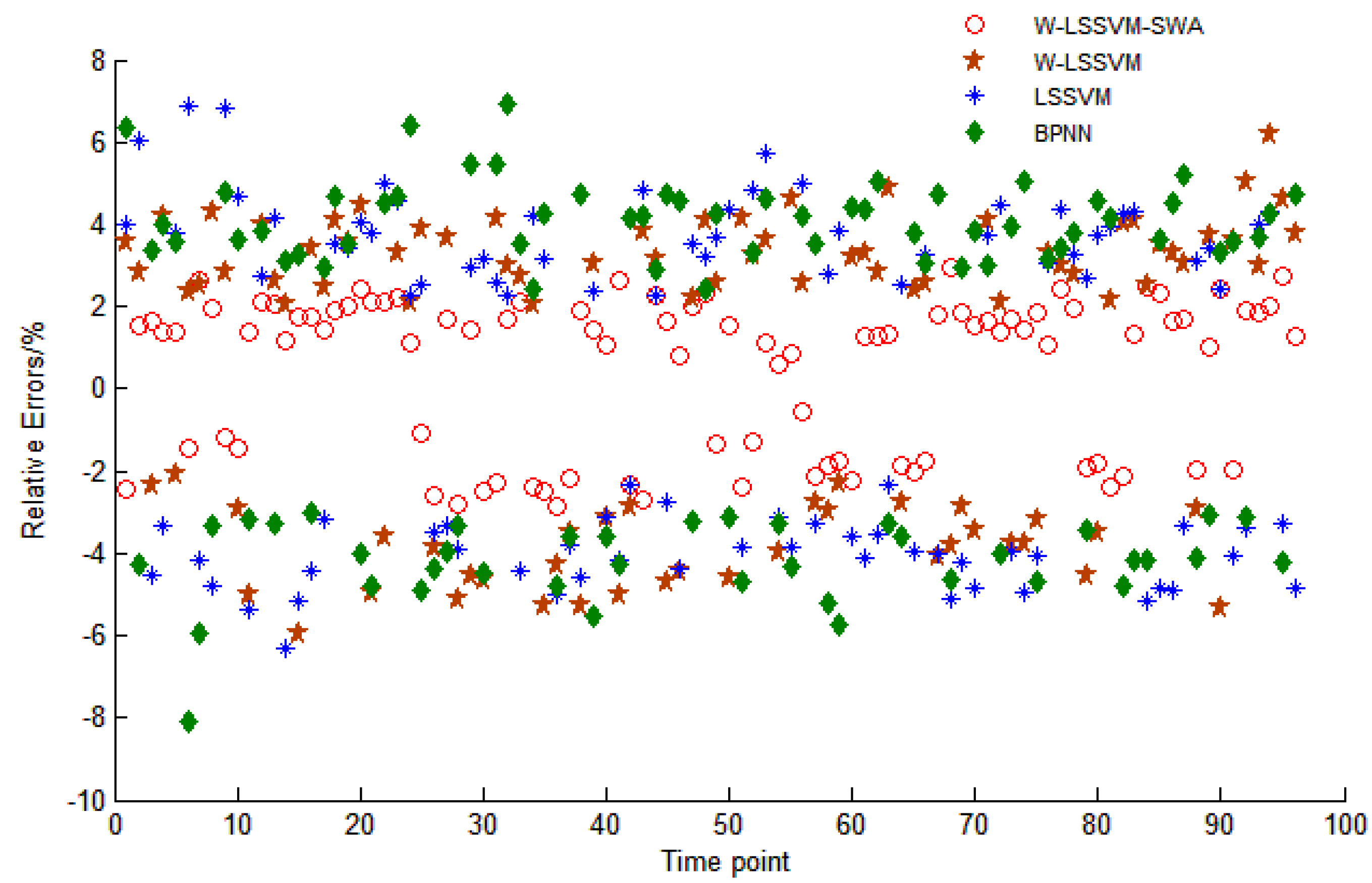
5.4. W-LSSVM for Load Forecasting

After all the optimal features of the sample data are obtained, the input vectors are brought into the W-LSSVM model for training and testing. This paper adopts independent program operation and calculation in the Matlab software. It should be noted that this paper chooses wavelet kernel function as the kernel function of the W-LSSVM regression model, and the important parameters of the model are obtained by QFA algorithm to optimize the process, to ensure the accuracy of the W-LSSVM model. The parameters of the SWA model are set as follows: the initial population number is 50, $m=10,n=5$, the initial reflection factor $c=2$, the contraction factor $r=0.95$, the number of GG individuals $q=4$, and the visual radius $Q=10$. The W-LSSVM model parameters calculated by running programs are $\gamma =36.5236$, $\sigma =12.1445$.

To prove the prediction performance of the forecasting model, this paper also selects the least squares support vector machine model (least square support vector machine, LSSVM), BP neural network model (BP neural networks, BPNN) and W-LSSVM model to predict the case, and evaluates and analyzes the prediction results of four models. In a single LSSVM prediction model, the selection of its parameters is as follows:

$$C=9.697,\epsilon =0.0017,\sigma =3.2361$$

In the BPNN prediction model, the neuron number of the input layer, hidden layer and output layer is set as 5, 7 and 1, respectively; the neuron activation function is Sigmoid function; the maximum allowable error of model training is 0.001; and the maximum number of iterations is set as 5000.

In the W-LSSVM model without parameter optimization, its parameter determination is obtained by cross validation, and its parameters are selected as follows:

$$C=18.248,\epsilon =0.0011,\sigma =4.257$$

Table 3. The forecasting results of each model.

Time Point	Actual	W-LSSVM-SWA		W-LSSVM		LSSVM		BPNN
		Forecast	Error	Forecast	Error	Forecast	Error	Forecast	Error
T00_00	80.23	78.28	−2.43%	83.12	3.60%	83.45	4.01%	85.32	6.34%
T01_00	80.23	81.33	1.37%	78.56	−2.09%	83.26	3.77%	83.10	3.58%
T02_00	81.04	80.07	1.20%	83.34	2.84%	86.56	6.81%	84.92	4.79%
T03_00	80.09	81.74	2.06%	82.19	2.62%	83.4	4.13%	77.45	−3.29%
T04_00	78.73	79.86	1.43%	80.68	2.47%	76.23	−3.18%	81.05	2.94%
T05_00	79.56	81.22	2.09%	75.6	−4.98%	82.58	3.80%	75.75	−4.79%
T06_00	81.52	80.63	−1.09%	84.7	3.90%	83.6	2.55%	77.53	−4.89%
T07_00	83.93	85.13	1.43%	80.14	−4.51%	86.4	2.94%	88.51	5.46%
T08_00	82.63	84.36	2.10%	84.88	2.73%	78.95	−4.45%	85.53	3.51%
T09_00	84.43	82.58	−2.19%	81.49	−3.48%	81.22	−3.80%	81.39	−3.59%
T10_00	85.32	87.56	2.62%	81.07	−4.98%	81.78	−4.15%	81.70	−4.25%
T11_00	86.65	88.06	1.63%	82.6	−4.67%	84.26	−2.76%	90.76	4.74%
T12_00	87.42	86.23	−1.36%	89.66	2.56%	90.65	3.69%	91.15	4.27%
T13_00	81.99	82.9	1.11%	84.98	3.65%	86.7	5.75%	85.76	4.60%
T14_00	82.37	80.62	−2.13%	80.1	−2.76%	79.69	−3.26%	85.27	3.52%
T15_00	83.87	84.96	1.30%	86.65	3.32%	80.42	−4.11%	87.55	4.39%
T16_00	84.81	83.09	−2.02%	86.85	2.41%	81.47	−3.93%	88.00	3.76%
T17_00	86.05	87.63	1.83%	83.6	−2.85%	82.44	−4.20%	88.59	2.95%
T18_00	88.19	89.7	1.71%	84.9	−3.73%	84.7	−3.96%	91.66	3.93%
T19_00	91.66	93.86	2.41%	94.4	2.99%	95.65	4.36%	94.80	3.43%
T20_00	91.91	89.72	−2.38%	93.9	2.16%	95.55	3.96%	95.72	4.15%
T21_00	88.53	90.6	2.34%	91.66	3.53%	84.25	−4.84%	91.74	3.63%
T22_00	86.78	87.64	0.99%	90.01	3.72%	89.74	3.41%	84.12	−3.06%
T23_00	83.06	84.6	1.86%	85.56	3.01%	86.36	3.98%	86.09	3.66%
MAPE			1.83%		3.57%		3.93%		4.15%
RMSE			0.0190		0.0369		0.0404		0.0426

and Figure 10 show the 96-point load forecasting results for 30 April 2016 with BPNN, LSSVM, W-LSSVM and W-LSSVM-SWA models. In addition, Figure 11 gives the forecasting errors with these models. Based on those forecasting results, several patterns are observed.

Firstly, the maximum and minimum gap between the original load value and forecasting load value are observed from Figure 10. With BPNN model, the maximum gap is 6.48 MW which is at 01:15, and the minimum gap is 2.01 MW which is at 08:15. In single LSSVM model, the maximum and minimum gaps are 5.52 MW and 1.85 MW, which are at 02:00 and 05:45, respectively. In W-LSSVM model, the maximum and minimum gaps are 5.06 MW and 1.64 MW, which are at 23:15 and 03:15, respectively. Both values of W-LSSVM are smaller than LSSVM and BPNN, which indicates the forecasting accuracy of W-LSSVM is more precise than that of BPNN and SVM. The results also demonstrate that the wavelet kernel function can improve the fitting and training ability of the LSSVM, which makes the algorithm have higher prediction accuracy.

With the new proposed W-LSSVM-SWA short-term power load forecasting system, the maximum and minimum forecasting gap are only 2.51 MW and 0.47 MW which are at 16:45 and 13:45, respectively. Both values of W-LSSVM-SWA are smaller that of BPNN, LSSVM and W-LSSVM. This illustrates that the proposed W-LSSVM-SWA model has a higher prediction accuracy and stability with the selection and extraction of candidate features by DWT-IR model, which improves the usability of input vector information and enhances the robustness of the algorithm.

Secondly, the relative errors between forecasting value and original value with these models can be described in Figure 11. Li and Guo et al. [17] regarded the error range (−3%, +3%) as a standard to judge the performance of the forecasting models. Therefore, this paper also uses this criterion to measure the performance of the proposed forecasting models. As we can see in Figure 11, the maximum and minimum relative errors of BPNN are 8.07% and 2.43%, respectively. Most RE values are out of the range (−3%, +3%); only five RE values are in this range, which demonstrates that the prediction effect of BPNN model is not ideal. With the LSSVM model, 15 relative errors are ranged in (−3%, +3%) and the rest of RE values are out of this range. Despite this, the LSSVM model has a better forecasting accuracy than the BPNN model. In addition, the maximum and minimum RE values of LSSVM model are 6.86% and 2.26%, both values of LSSVM model are smaller than that of BPNN, which again demonstrate the LSSVM has a better prediction accuracy. In W-LSSVM model, the maximum and minimum RE values are 6.18% and 2.06%, which are smaller than that of LSSVM and BPNN models. This directly demonstrates the prediction accuracy of W-LSSVM model is higher than that LSSVM and BPNN. Furthermore, 32 of RE values of W-LSSVM model are ranged in (−3%, +3%), and the RE values in this range is more than the LSSVM and BPNN model. This demonstrates that the W-LSSVM model has a good prediction effect for the short-term load forecasting, but it is not good enough and it needs further improvement. With the new proposed W-LSSVM-SWA short-term forecasting model, the maximum and minimum RE values are 2.93% and 0.57%, respectively. Both values of W-LSSVM-SWA model are superior to the BPNN, LSSVM and W-LSSVM model. In addition, all the RE values are in the range of (−3%, +3%), i.e., none of them are out of the range, which demonstrates the proposed W-LSSVM-SWA model has higher prediction accuracy than the other three models in solving short-term power load forecasting problem, and the predictive stability of W-LSSVM-SWA model is more higher among these four models.

Thirdly, the MAPE value and RMSE value of each model can be calculated from Table 3. As the calculation results shown, the proposed W-LSSVM-SWA forecasting model has higher forecast precision. Evidently, the MAPE value of the proposed model is 1.83%, which is obviously lower than the other models. In addition, the MAPE value of W-LSSVM model is 3.57%, which is lower than that of LSSVM model and BPNN model. The result also proves that the W-LSSVM model improves the fitting and learning ability by replacing the kernel function of the LSSVM model. In LSSVM model, the MAPE value is 3.93%, which is slightly lower than that of BPNN model (4.15%), this demonstrates that the LSSVM model can better gain the useful information from the sample data, and its fitting ability is stronger than the BPNN model in solving the problem of short-term power load forecasting.

RMSE is used to measure the deviation between the observed value and the true value. The smaller the RMSE value is, the higher the accuracy the model achieves. The RMSE values of the W-LSSVM-SWA, W-LSSVM, LSSVM and BPNN model are 1.90%, 3.69%, 4.04% and 4.26%, respectively. The RMSE value of W-LSSVM-SWA is the lowest among the four model, this illustrates that the W-LSSVM-SWA model has higher forecasting stability and accuracy, and the proposed model can reduce the redundant influence of irrelevance factors by DWT-IR model for the feature selection.

Furthermore, to identify the statistical significance of SWA optimization algorithm, this paper also compares the forecasting performances among the proposed W-LSSVM-SWA model, PSO-LSSVM model, GA-LSSVM model and ACO-LSSVM model. First the SWA optimization efficiency is compared with other optimization algorithms such as PSO, GA and ACO. The relative comparison results are presented in

Table 4. The results comparison for different algorithms.

Algorithm	Optimal Fitness Value	Accuracy	$\mathit{C}$	$\mathit{\sigma }$	Running Time/s
SWA	−0.764	98.98%	36.5236	12.1445	187
PSO	−0.733	97.5%	21.3857	9.6840	235
GA	−0.728	96.9%	24.5852	17.9034	244
ACO	−0.736	97.2%	10.1245	8.8789	212

. Part of forecasting results of W-LSSVM-SWA, PSO-LSSVM, GA-LSSVM and ACO-LSSVM models are shown in

Table 5. Forecasting results of each model (Unit: MW).

Time	Actual	W-LSSVM-SWA	PSO-LSSVM	GA-LSSVM	ACO-LSSVM
T12_00	87.42	86.23	88.72	85.14	84.78
T13_00	81.99	82.9	83.35	83.66	83.55
T14_00	82.37	80.62	83.67	80.25	80.69
T15_00	83.87	84.96	85.39	85.63	85.85
T16_00	84.81	83.09	85.79	86.35	84.89
T17_00	86.05	87.63	87.81	84.07	87.56
T18_00	88.19	89.7	89.82	87.24	90.65
T19_00	91.66	93.86	94.23	94.07	93.96
T20_00	91.91	89.72	93.67	92.86	90.43
T21_00	88.53	90.6	90.85	91.5	91.23
T22_00	86.78	87.64	88.23	88.54	88.79
T23_00	83.06	84.6	85.05	84.84	84.51
MAPE		1.83%	1.95%	2.16%	2.11%
RMSE		0.0190	0.0201	0.2281	0.2232

. As we can see in Table 4, all the optimization algorithms can achieve excellent prediction accuracy, but the parameters values of $C$ and $\sigma$ are not the same, and this could directly lead to different fitnesses. The optimal fitness value of SWA is the best and its running time is shortest. The optimal values of PSO-LSSVM, GA-LSSVM and ACO-LSSVM have little difference; however, due to the complexity of GA, its fitness is the worst and its execution time is the longest. This result demonstrates that SWA can help to improve the prediction accuracy and greatly reduce the running time for finding the optimal parameters of LSSVM.

It also can be seen from Table 5, the MAPE value of W-LSSVM-SWA, PSO-LSSVM, GA-LSSVM and ACO-LSSVM are 1.83%, 1.95%, 2.16% and 2.11%, respectively. This again demonstrates the SWA algorithm has better prediction performance and stronger applicability compared with other three algorithms. In addition, the RMSE value can explain a significant difference between the actual value and predictive value. The RMSE vale of W-LSSVM-SWA, PSO-LSSVM, GA-LSSVM and ACO-LSSVM are 0.0190, 0.0201, 0.2281 and 0.2232, respectively. The RMSE value of W-LSSVM-SWA is the smallest, and this illustrates the significance difference of W-LSSVM-SWA model is the smallest when compared with other three models. Based on those calculation results, it is obvious that the predictive performance of W-LSSVM-SWA has better universality and applicability.

In summary, the proposed W-LSSVM-SWA can reduce the forecasting errors between original power load values and predictive values. It can reduce the influence of unrelated noises with feature selection based on DWT-IR model. The LSSVM model improves its nonlinear mapping ability by using the wavelet kernel function, and its training and learning ability has been strengthen very well in this way. The numerical experimental results have demonstrated the feasibility and effectiveness of the proposed W-LSSVM-SWA short-term power load forecasting method.

6. Conclusions

This paper proposed a short-term load forecasting system based on wavelet least square support vector machine (W-LSSVM) and sperm whale algorithm (SWA). To establish this forecast method, the discrete wavelet transform and the inconsistency rate are combined for the feature selection, which aims to reduce the redundancy of input vectors in short-term load forecasting. In order to improve the learning and nonlinear mapping ability of LSSVM model, the wavelet kernel function is used to replace the Gaussian kernel function, thus the W-LSSVM model is established for the regression calculation. Furthermore, the parameters of W-LSSVM model are optimized by the sperm whale algorithm, which aims to improve the fitting ability and robustness of W-LSSVM model. The proposed method has been applied to the real-world load forecasting case, and the relevant results show that the proposed W-LSSVM-SWA method has ability to find the optimal feature subset and reach the expected forecast accuracy. The proposed short-term load forecasting method of W-LSSVM-SWA is effective and feasible, it may be an effective alternative for the short-term load forecasting in the integrated energy system.

References

1. Okabe, T.H.; Kuzmina, O.; Slattery, J.M.; Jiang, C.; Sudmeier, T.; Yu, L.; Wang, H.; Xiao, W.; Xu, L.; Yue, X.; et al. Benefits to energy efficiency and environmental impact: General discussion. Faraday Discuss. 2016, 190, 161–204. [Google Scholar] [CrossRef] [PubMed]
2. Wang, W.; Wang, D.; Jia, H.; Chen, Z.; Guo, B.; Zhou, H.; Fan, M. Review of steady-state analysis of typical regional integrated energy system under the background of energy internet. Proc. CSEE 2016, 36, 3292–3306. [Google Scholar]
3. Wu, J. Drivers and state-of-the-art of integrated energy systems in Europe. Autom. Electr. Power Syst. 2016, 40, 1–7. [Google Scholar]
4. Clements, A.E.; Hurn, A.S.; Li, Z. Forecasting day-ahead electricity load using a multiple equation time series approach. Eur. J. Oper. Res. 2014, 251, 522–530. [Google Scholar] [CrossRef]
5. Cui, H.; Peng, X.; Mu, Y. Electric load forecast using combined models with HP Filter-SARIMA and ARMAX optimized by regression analysis algorithm. Math. Probl. Eng. 2015, 2015, 326925. [Google Scholar]
6. Zhao, H.; Guo, S. An optimized grey model for annual power load forecasting. Energy 2016, 107, 272–286. [Google Scholar] [CrossRef]
7. Coelho, V.N.; Coelho, I.M.; Coelho, B.N.; Reis, A.J.R.; Enayatifar, R.; Souza, M.J.F.; Guimarães, F.G. A self-adaptive evolutionary fuzzy model for load forecasting problems on smart grid environment. Appl. Energy 2016, 169, 567–584. [Google Scholar] [CrossRef]
8. Hernandez, L.; Baladrón, C.; Aguiar, J.M.; Carro, B.; Sanchez-Esguevillas, A.J.; Lloret, J. Short-term load forecasting for microgrids based on artificial neural networks. Energies 2013, 6, 1385–1408. [Google Scholar] [CrossRef]
9. Dudek, G. Neural networks for pattern-based short-term load forecasting: A comparative study. Neurocomputing 2016, 205, 64–74. [Google Scholar] [CrossRef]
10. Rana, M.; Koprinska, I. Forecasting electricity load with advanced wavelet neural networks. Neurocomputing 2016, 182, 118–132. [Google Scholar] [CrossRef]
11. Hu, R.; Wen, S.; Zeng, Z.; Huang, T. A short-term power load forecasting model based on the generalized regression neural network with decreasing step fruit fly optimization algorithm. Neurocomputing 2016, 221, 24–31. [Google Scholar] [CrossRef]
12. Pan, X.; Lee, B. A comparison of support vector machines and artificial neural networks for mid-term load forecasting. In Proceedings of the IEEE International Conference on Industrial Technology, Athens, Greece, 19–21 March 2012; pp. 95–101. [Google Scholar]
13. Ceperic, E.; Ceperic, V.; Baric, A. A strategy for short-term load forecasting by support vector regression machines. IEEE Trans. Power Syst. 2013, 28, 4356–4364. [Google Scholar] [CrossRef]
14. Pai, P.F.; Hong, W.C. Forecasting regional electricity load based on recurrent support vector machines with genetic algorithms. Electr. Power Syst. Res. 2005, 74, 417–425. [Google Scholar] [CrossRef]
15. Ren, G.; Wen, S.; Yan, Z.; Hu, R.; Zeng, Z.; Cao, Y. Power load forecasting based on support vector machine and particle swarm optimization. In Proceedings of the 2016 12th World Congress on Intelligent Control and Automation, Guilin, China, 12–15 June 2016; pp. 2003–2008. [Google Scholar]
16. Zhang, X.; Wang, J.; Zhang, K. Short-term electric load forecasting based on singular spectrum analysis and support vector machine optimized by Cuckoo search algorithm. Electr. Power Syst. Res. 2017, 146, 270–285. [Google Scholar] [CrossRef]
17. Li, H.; Guo, S.; Zhao, H.; Su, C.; Wang, B. Annual electric load forecasting by a least squares support vector machine with a fruit fly optimization algorithm. Energies 2012, 5, 4430–4445. [Google Scholar] [CrossRef]
18. Niu, D.; Ma, T.; Liu, B. Power load forecasting by wavelet least squares support vector machine with improved fruit fly optimization algorithm. J. Comb. Optim. 2016, 33, 1122–1143. [Google Scholar]
19. Sun, W.; Liang, Y. Least-squares support vector machine based on improved imperialist competitive algorithm in a short-term load forecasting model. J. Energy Eng. 2014. [Google Scholar] [CrossRef]
20. Liang, Y.; Niu, D.; Ye, M.; Hong, W.C. Short-term load forecasting based on wavelet transform and least squares support vector machine optimized by improved cuckoo search. Energies 2016, 9, 827. [Google Scholar] [CrossRef]
21. Du, J.; Liu, Y.; Yu, Y.; Yan, W. A prediction of precipitation data based on support vector machine and particle swarm optimization (PSO-SVM) algorithms. Algorithms 2017, 10, 57. [Google Scholar] [CrossRef]
22. Cai, G.; Wang, W.; Lu, J. A novel hybrid short term load forecasting model considering the error of numerical weather prediction. Energies 2016, 9, 994. [Google Scholar] [CrossRef]
23. Ye, F.; Lou, X.Y.; Sun, L.F. An improved chaotic fruit fly optimization based on a mutation strategy for simultaneous feature selection and parameter optimization for SVM and its applications. PLoS ONE 2017, 12, e0173516. [Google Scholar] [CrossRef] [PubMed]
24. Zhang, X.L.; Chen, X.F.; He, Z.J. An ACO-based algorithm for parameter optimization of support vector machines. Expert Syst. Appl. 2010, 37, 6618–6628. [Google Scholar] [CrossRef]
25. Ebrahimi, A.; Khamehchi, E. Sperm whale algorithm: An effective metaheuristic algorithm for production optimization problems. J. Nat. Gas Sci. Eng. 2016, 29, 211–222. [Google Scholar] [CrossRef]
26. Gorjaei, R.G.; Songolzadeh, R.; Torkaman, M.; Safari, M.; Zargar, G. A novel PSO-LSSVM model for predicting liquid rate of two phase flow through wellhead chokes. J. Nat. Gas Sci. Eng. 2015, 24, 228–237. [Google Scholar] [CrossRef]
27. Ahmadi, M.A.; Bahadori, A. A LSSVM approach for determining well placement and conning phenomena in horizontal wells. Fuel 2015, 153, 276–283. [Google Scholar] [CrossRef]
28. Nieto, P.G.; García-Gonzalo, E.; Fernández, J.A.; Muñiz, C.D. A hybrid wavelet kernel SVM-based method using artificial bee colony algorithm for predicting the cyanotoxin content from experimental cyanobacteria concentrations in the Trasona reservoir (Northern Spain). J. Comput. Appl. Math. 2016, 309, 587–602. [Google Scholar] [CrossRef]
29. Makbol, N.M.; Khoo, B.E. Robust blind image watermarking scheme based on Redundant Discrete Wavelet Transform and Singular Value Decomposition. AEU—Int. J. Electron. Commun. 2013, 67, 102–112. [Google Scholar] [CrossRef]
30. Giri, D.; Acharya, U.R.; Martis, R.J.; Sree, S.V.; Lim, T.C.; Ahamed, T.; Suri, J.S. Automated diagnosis of Coronary Artery Disease affected patients using LDA, PCA, ICA and Discrete Wavelet Transform. Knowl.-Based Syst. 2013, 37, 274–282. [Google Scholar] [CrossRef]
31. Salas-Boni, R.; Bai, Y.; Harris, P.R.E.; Drew, B.J.; Hu, X. False ventricular tachycardia alarm suppression in the ICU based on the discrete wavelet transform in the ECG signal. J. Electrocardiol. 2014, 47, 775–780. [Google Scholar] [CrossRef] [PubMed]
32. Chhabra, L.; Flynn, A.W. Inconsistency of hemodynamic data in severe aortic stenosis: Yet unexplored reasoning! Int. J. Cardiol. 2016, 67, 2446–2447. [Google Scholar] [CrossRef] [PubMed]
33. Pfeifer, M. Different outcomes of meta-analyses and data inconsistency. Osteoporos. Int. 2015, 26, 1–2. [Google Scholar] [CrossRef] [PubMed]
Figure 1. Grouping process in sperm whale algorithm (SWA).
Sustainability 09 01188 g001
Figure 2. Reflection of worse answer in SWA.
Sustainability 09 01188 g002
Figure 3. Calculation process of SWA.
Sustainability 09 01188 g003
Figure 4. Discrete wavelet transformation structure.
Sustainability 09 01188 g004
Figure 5. A flowchart of the QFA-W-LSSVM framework for icing forecasting.
Sustainability 09 01188 g005
Figure 6. The distribution of training dataset from 21 March 2015 to 24 April 2016.
Sustainability 09 01188 g006
Figure 7. The distribution of testing dataset from 24 April 2016 to 30 April 2016.
Sustainability 09 01188 g007
Figure 8. The box-plot of training and testing dataset.
Sustainability 09 01188 g008
Figure 9. The curve of convergence for feature selection.
Sustainability 09 01188 g009
Figure 10. The forecasting values of each model.
Sustainability 09 01188 g010
Figure 11. The relative errors of each forecasting model.
Sustainability 09 01188 g011