Velocity Obstacle Based 3D Collision Avoidance Scheme for Low-Cost Micro UAVs

Abstract

An unmanned aerial vehicle (UAV) must be able to safely reach its destination even, when it can only gather limited information about its environment. When an obstacle is detected, the UAV must be able to choose a path that will avoid collision with the obstacle. For the collision avoidance scheme, we apply the velocity obstacle approach since it is applicable even with the UAV’s limited sensing capability. To be able to apply the velocity obstacle approach, we need to know the parameter values of the obstacle such as its size, current velocity and current position. However, due to the UAV’s limited sensing capability, such information about the obstacle is not available. Thus, by evaluating sensor readings, we get the changes in the possible positions of the obstacle in order to generate the velocity obstacle and make the UAV choose a collision-free trajectory towards the destination. We performed simulation on different obstacle movements and the collision-free trajectory of the UAV is shown in the simulation results.

1. Introduction

Many studies have focused on the full automation of low-cost unmanned aerial vehicles (UAVs). The interest on UAV has increased due to its high applicability in various areas such as law enforcement, search and rescue, agriculture monitoring, and weather monitoring. One topic in such studies is the collision avoidance system for fully automated UAVs.

This problem is applicable to the field of networking when UAVs are used for information delivery. A communication network must be established using multiple UAVs with limited communication range [1,2,3]. In similar applications, two UAVs that need to exchange information are separated beyond the communication range. Thus, the UAVs are required to travel between each other’s communication range [3]. In such environment, UAV may be instructed to deliver information as quickly as possible to the appropriately chosen UAV, avoiding obstacles efficiently on the path to the target UAV.

The sensing and detection capability, and the collision avoidance approach are two of the main issues for a collision avoidance system [4]. Various sensors are used by different studies on the collision avoidance of UAVs. ADS-B sensors, a surveillance technology that enables the UAV to keep track of information of other UAVs, are used in [5,6,7]. For collision avoidance, Fu et al. [5] used differential geometric guidance and flatness techniques for collision avoidance; Park et al. [6] proposed the concept of Vector sharing; and Lin and Saripalli [7] proposed the concept of reachable sets. In [8,9,10,11,12], vision based approach is used for obstacle detection. A Doppler radar sensor is used in [13] for obstacle detection and a reactive collision avoidance algorithm is developed. In [14], a fusion of ultrasonic sensor and infrared sensor is used for increased accuracy of sensor measurements, which is then input to a collision avoidance controller. Other types of sensors are small sized radar sensor [15], optic-flow sensor [16], and Ultra-wideband sensor [17].

The main focus of this paper is to devise a collision avoidance scheme using only the distance information of the obstacle. Our work is based on the simple modeling of low-cost micro UAV with limited sensing capability. Accordingly, it does not model the dynamics of the system and does not take into account the noisy environment in sensing the obstacle. The UAV must be able to safely reach its destination provided it can only gather limited information about its environment. We apply the velocity obstacle approach introduced in [18] to be able to determine the possible maneuvers that the UAV can take to avoid collision. However, because of the sensing limitation, we need to determine the unavailable parameter values of the obstacle. The concept of velocity obstacle is also used in [19,20]. In [19], reciprocal collision avoidance is introduced. Reciprocal collision avoidance considers the navigation of many agents and in which each agent applies the velocity obstacle approach. In [20], the implementation of reciprocal collision avoidance on real quadrotor helicopters is presented. Contrary to this paper, the sensing capability is not an issue in [18,19,20]. In this paper, we show how to overcome the UAV’s limited sensing capability to be able to find a collision-free trajectory to the goal with the use of the velocity obstacle approach.

This paper is organized as follows: In Section 2, related works on collision-free trajectory planning of UAVs are discussed. In Section 3, the set-up model of the UAV is defined. Section 4 briefly explains the concept of velocity obstacle. Section 5 shows our approach on using velocity obstacle with limited obstacle information. Section 6 presents the summary of collision avoidance algorithm. The simulation results and discussion are presented in Section 7. Finally, Section 8 concludes the paper.

2. Related Work

Various approaches have been proposed and implemented on the problem of collision-free autonomous flight of UAVs. Certainly, different approaches have different system models and different assumptions on the available information about the environment. Rapidly exploring random tree is used in [21,22] to generate feasible trajectories of the UAV. A tree representing the feasible trajectories of the UAV, with nodes as the waypoints, is made and the node sequence with the smallest cost is chosen as the final path. In [21], a sampling based method is used with a closed-loop rapidly exploring random tree while path planning based on 3D Dubins curve is used in [22].

A model predictive control is used in [23] for generating the UAV’s trajectory. They presented the formulation of the MPC-based approach with consideration to the dynamic constraints. It is modeled in a dual-mode strategy defined by the normal flight mode and the evasion mode. In a normal flight mode, the model chooses a parameter that will provide stability to the UAV and also improves its performance. Once an obstacle’s trajectory is predicted, it will switch to evasion mode with the goal of avoiding the obstacle. It is assumed that the UAV has onboard sensors that provide information of the obstacle. Bai et al. [24] used partially observable Markov decision process (POMDP) to model the collision avoidance system. POMPD is solved by applying Monte Carlo Value Iteration (MCVI) algorithm that computes the policy with maximal total reward. Total field sensing approach is applied in [25]. It allows multiple vehicles to travel to each of its goal. This approach uses the magnetic field theory. Basically, each vehicle has a magnet that generates its magnetic field and has magnetic sensors that detect the total field from other vehicles. The gradient of the total field is estimated and the vehicle moves away from the direction of the gradient to avoid collision. Frew and Sengupta’s approach [26] is based on the concept of reachable sets. The backwards reachable sets (BRS) is defined as the set of states of the system that will lead the UAV to the obstacle. The formation planner must generate the feasible avoidance maneuver before the UAV enters the boundary of the BRS. Two-camera and parallel-baseline stereo are used to determine the position of the obstacles.

A simple reactive collision avoidance is used in [13]. Doppler radars are used to sense the environment. The radar return with higher magnitude means that it has more or larger obstacles. The reactive algorithm will then choose the path with lowest return radar signal. Another reactive obstacle collision avoidance algorithm is used in [27]. It is a map-based approach wherein a 3D occupancy map represents the environment and is improved for every obstacle detection so that the previous detections can be considered when deciding the next waypoint. When an obstacle is detected, an escape point search algorithm is used to find a waypoint that is reachable from the UAV’s current position and at the same time avoids the obstacle. The UAV will then move towards the goal after the waypoint is reached. Combined stereo and laser-based sensing is used to sense the environment. A map-based approach is also used in [28] using a grid-based map of probability of threats. From the sensor readings, Bayes’ rule is applied to get the occupancy values of the cell. Preliminary path planning is done based on the initial information on the location of the obstacles. When an unexpected obstacle is detected, the probabilities are updated.

3. Environment Model

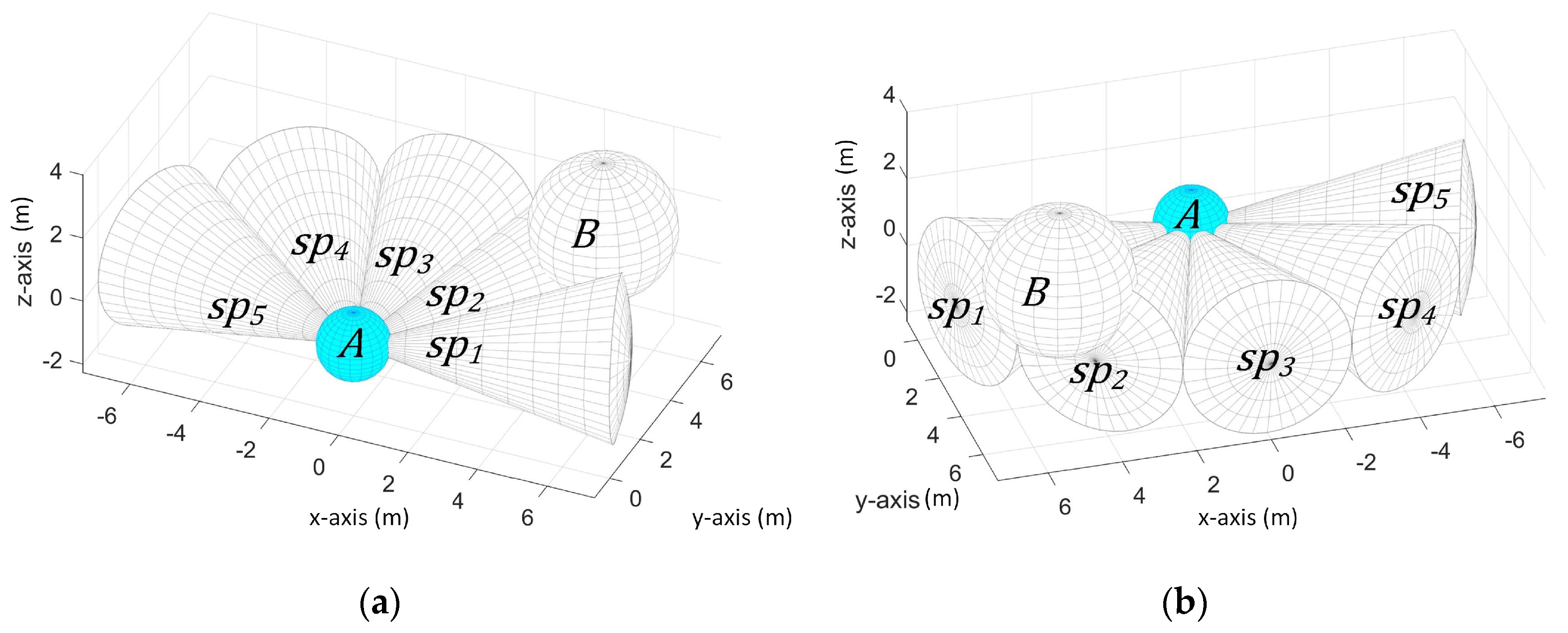
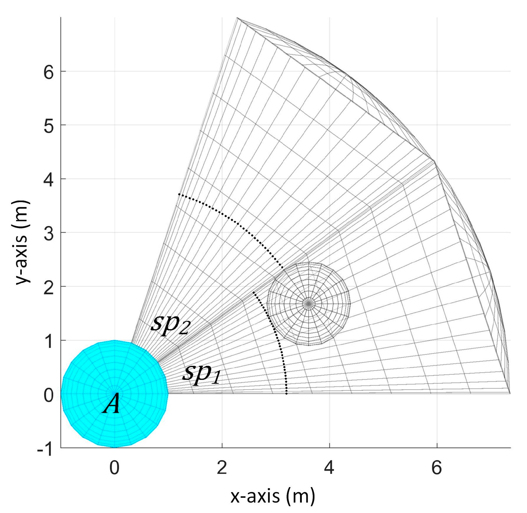
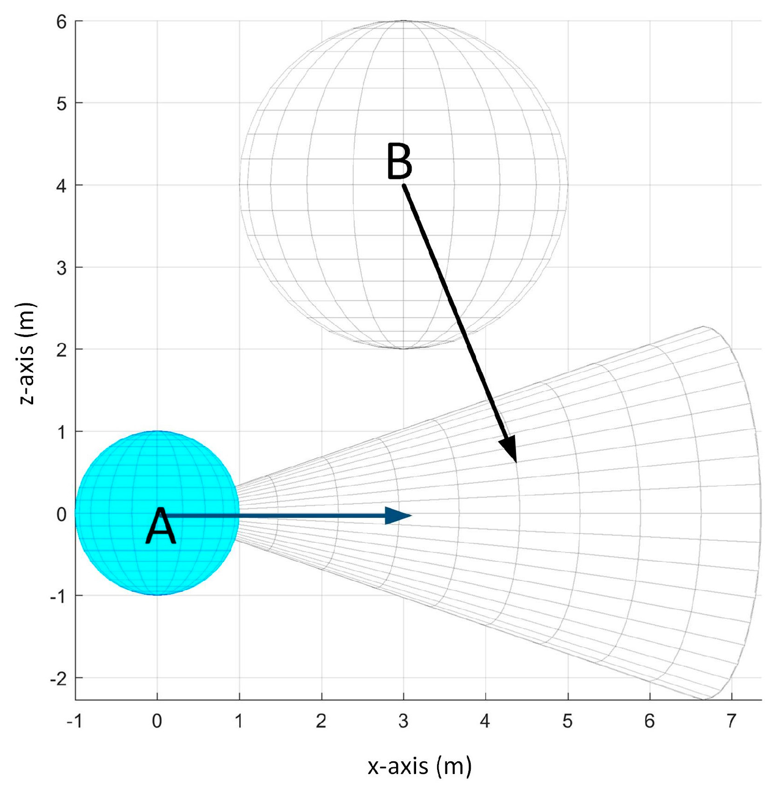
We consider a UAV and an obstacle that share an environment in a 3-D space. The UAV must arrive at the goal destination while avoiding collision with the obstacle. Let there be two spherical objects $A$ and $B$ as the UAV and the obstacle respectively as shown in Figure 1. Figure 1a shows the view from the back of $A$ and Figure 1b shows the view from the front. The UAV has five ultrasonic sensors whose sensing space is spherical sector shaped with a default opening angle of 36 degrees and a maximum detection range of 7 to 10 m each. The sensors are attached at the front of the UAV and their orientation is shown in Figure 1. In this figure, $A$ is positioned at (0, 0, 0) and $B$ is at the upper-right-front of $A$. The sensors are labeled in counter-clockwise direction. $s{p}_s$ denotes the sensing space of sensor $S\in \left\{1,2,3,4,5\right\}$ and $d_s$ denotes the sensor reading of sensor $S$ which is the nearest distance of the obstacle from the UAV within the detection range of $S$.

The UAV has a fixed radius $r_A$, its current center position $p_A$, and current velocity $v_A$. The obstacle also has a fixed radius $r_B$, its current center position $p_B$, and current velocity $v_B$. $r_B$, $p_B$, and $v_B$ are unknown to the UAV due to the limitation of its sensors. $d_s$ is the only available information to the UAV.

Aside from the limitation that it can only provide the nearest distance value of the obstacle, another limitation in this setup is the limited sensor range in the x-z plane and y-z plane. In the x-y plane, we have a total of 180 degree of sensing range and each sensor covers different sensing space region. Thus, we can determine the vicinity of the location of the obstacle only in the x-y plane. For example, if the obstacle is detected by sensor 1, then we know that the obstacle is somewhere in the right-front part of the UAV in x-y plane when the UAV is facing along the y-axis. However, we cannot know whether its position is higher or lower than the UAV because the positioning of the sensors provides limited view of the UAV’s environment in the x-z plane and y-z plane.

4. Velocity Obstacle

We apply the method of using velocity obstacle [18] in choosing the velocity that the UAV would take. Using velocity obstacle, we can determine the possible velocities the UAV can take that will avoid collision with the obstacle. This approach is simple and the velocity obstacle can be calculated given the basic information of the obstacle and the UAV. We will briefly discuss the concept of velocity obstacle and how it is applied to this paper.

The velocity obstacle $V{O}_{A|B}$ is the set of all velocities of $A$ that will result in a collision to $B$ at some future time assuming that $B$ maintains a constant velocity $v_B$. A geometric interpretation of $V{O}_{A|B}$ is shown in Figure 2. Let $A\oplus B$ be the Minkowski sum of $A$ and $B$, let $-A$ denote $A$ reflected in its reference point and let $\mathsf{\lambda }\left(p,v\right)$ be the ray starting at position $p$ with direction $v$:

$$A\oplus B=\{a+b|a\in A,bϵB\}$$

(1)

$$-A=\{-a|aϵA\}$$

(2)

$$\lambda \left(p,v\right)=\{p+tv|t\ge 0\}$$

(3)

We now define $V{O}_{A|B}$ as:

$$V{O}_{A|B}=\left\{v_A\right|\lambda \left(p_A,v_A-v_B\right){\displaystyle \bigcap }B\oplus -A\ne \varnothing \}$$

(4)

which means that choosing $v_A$ inside $V{O}_{A|B}$ will result to collision between $A$ and $B$ at some future time. While selecting $v_A$ outside $V{O}_{A|B}$ would avoid collision with $B$.

This concept is discussed in 2D but can be easily extended to 3D by considering spheres instead of circles and adding the lines tangent to the upper and lower part of the obstacle as shown in Figure 3.

5. Generating Velocity Obstacle Based on the Estimated Parameter Values of the Obstacle

As explained in the previous section, applying the velocity obstacle approach requires the parameter values $r_B$, $p_B$, and $v_B$. However, due to the limitation of the sensors, we only have limited information about the obstacle; that is, we only have $d_s$. Thus, from our only available information $d_s$, we get the possible values of $r_B$, $p_B$, and $v_B$. Afterwards, the possible $V{O}_{A|B}$ can be created based on the computed possible values of $r_B$, $p_B$, and $v_B$. In the following subsections, we discuss how we derive these values.

On the whole, the behavior of our system is as follows: For each time step interval $t_i$, $d_s$ is provided. Then the possible values of $r_B$, $p_B,$ $v_B$, and $V{O}_{A|B}$ are computed sequentially based on $d_s$ at every $t_i$. Lastly, $v_A$ for this $t_i$ is chosen based on the generated possible $V{O}_{A|B}$s.

In addition, we have two possible cases when the obstacle is detected as defined below:

Case 1

Obstacle’s center is inside sensor’s detection range

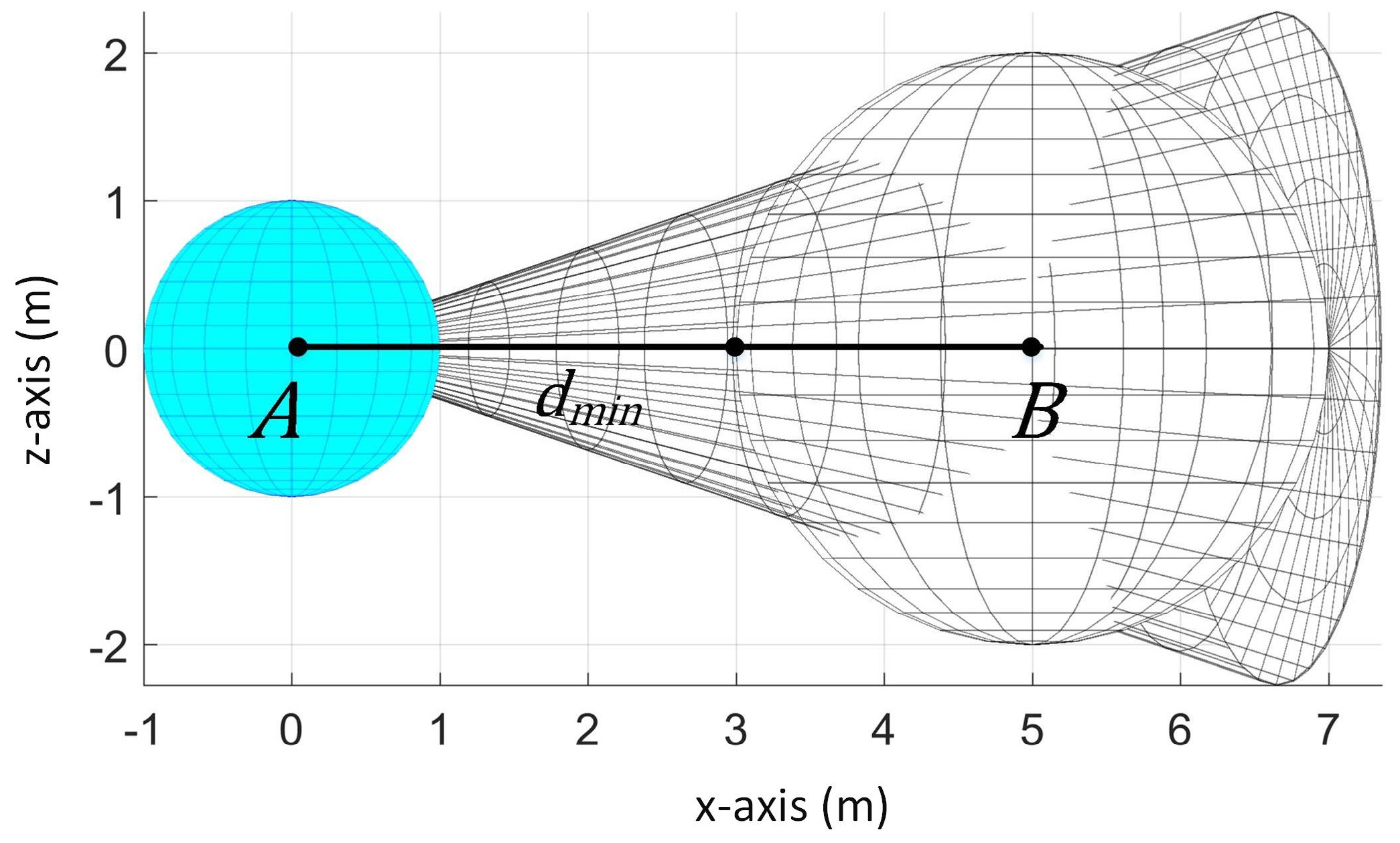
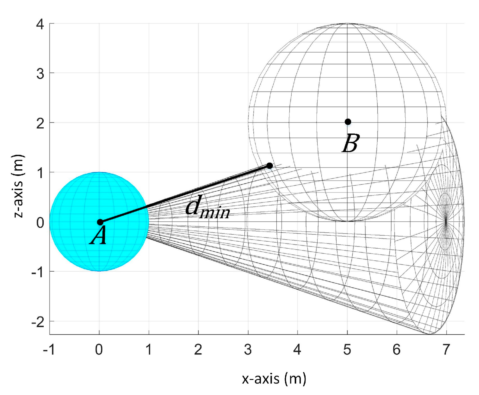
• When the obstacle’s center is inside the sensor’s detection range, then the minimum $d_s$ denoted as $d_{min}$ is measured along the line connecting the center of $A$ and the center of $B$ as shown in Figure 4. Thus, the following equation holds in this scenario:

  $$dist\left(p_A,p_B\right)=d_{min}+r_B$$

  (5)

  where $dist\left(x,y\right)$ denotes the distance between points $x$ and $y$.
• Then, we can use $d_{min}$ to get the possible values of $r_B$, $p_B,$ and $v_B$ since we can assume that obstacle is positioned inside the sensor’s detection range.

Case 2

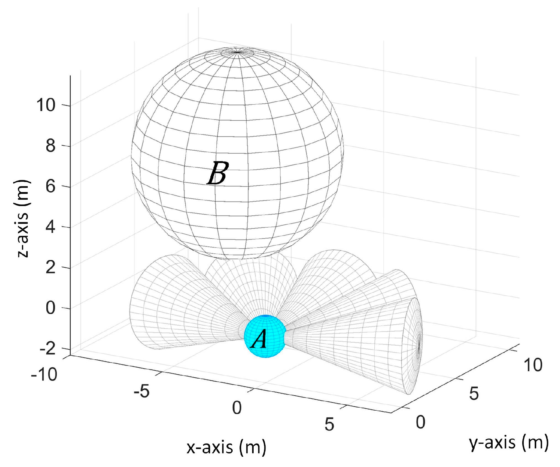
Obstacle’s center is not inside sensor’s detection range

• When the obstacle’s center is not inside the sensor’s detection range and it is at the upper or lower part of the sensing space, as seen in Figure 5, $d_{min}$ is not measured along the line connecting the center of the UAV and the center of obstacle but it is at the closest point from the center of the UAV to the surface of the obstacle that intersected with the sensing space.
• In this case, Equation (5) does not hold and we cannot generate correct possible values of $r_B$, $p_B,$ and $v_B$.

Due to the limitation in the sensing capability, we cannot recognize whether the obstacle’s actual center position belongs to Case 1 or Case 2 by knowing only $d_s$. This is taken into account in determining the obstacle’s possible sizes, positions, and velocities. For the obstacle’s size, its maximum possible radius is predetermined since this cannot be determined when it belongs to Case 2. For the obstacle’s position, we get its extreme possible center positions for the cases when the obstacle’s center is inside and outside the detection space. Then, we get the differences of the computed possible positions between two consecutive time steps to get its possible velocities. We further discuss this in the following subsections.

5.1. Computing Obstacle’s Possible Radius

We are interested in getting the obstacle’s smallest and biggest possible radii. Ideally, we want to determine the lower bound $l{r}_B$ and upper bound $u{r}_B$ of the radius based on $d_{min}$. However, as mentioned previously, we cannot use $d_{min}$ to determine required information on the obstacle when the obstacle belongs to Case 2. Unfortunately, given only $d_s$, we cannot know which case the obstacle belongs to because of the limited sensing view in the x-z and y-z plane. Figure 6 shows an example of this problem. This shows that because of the limited sensing view in x-z and y-z plane, when an obstacle belongs to Case 2, it is possible that the obstacle is detected by only one sensor even though the obstacle is big. Considering this case, $u{r}_B$ should be infinitely big for our $u{r}_B$ to be always accurate. However, it is possible in other scenarios that the obstacle is actually small enough that it is always detected by one sensor. Thus, we cannot let $u{r}_B$ be infinitely big because this also makes the velocity obstacle very big and in effect will limit the possible paths the UAV can take, even though the obstacle is actually small. To address this limitation in our sensing capability, we are forced to assign a fixed value to the $u{r}_B$ in order for the UAV to still be able to find possible paths that are outside the velocity obstacle. Hence, $u{r}_B=r_{B,max}$ where $r_{B,max}$ is a predetermined obstacle’s maximum possible radius.

Thus, we only compute $l{r}_B$ and we compute it every time step to be able to continually improve it. That means, if the new $l{r}_B$ is bigger than the existing $l{r}_B$, then we replace the existing $l{r}_B$ with the new $l{r}_B$. For $u{r}_B$, it has fixed user-defined value for all of the time steps. Our approach is not applicable for multiple obstacles since it assumes that the obstacle that will be detected in the future time steps is the same obstacle that is detected in the current time step.

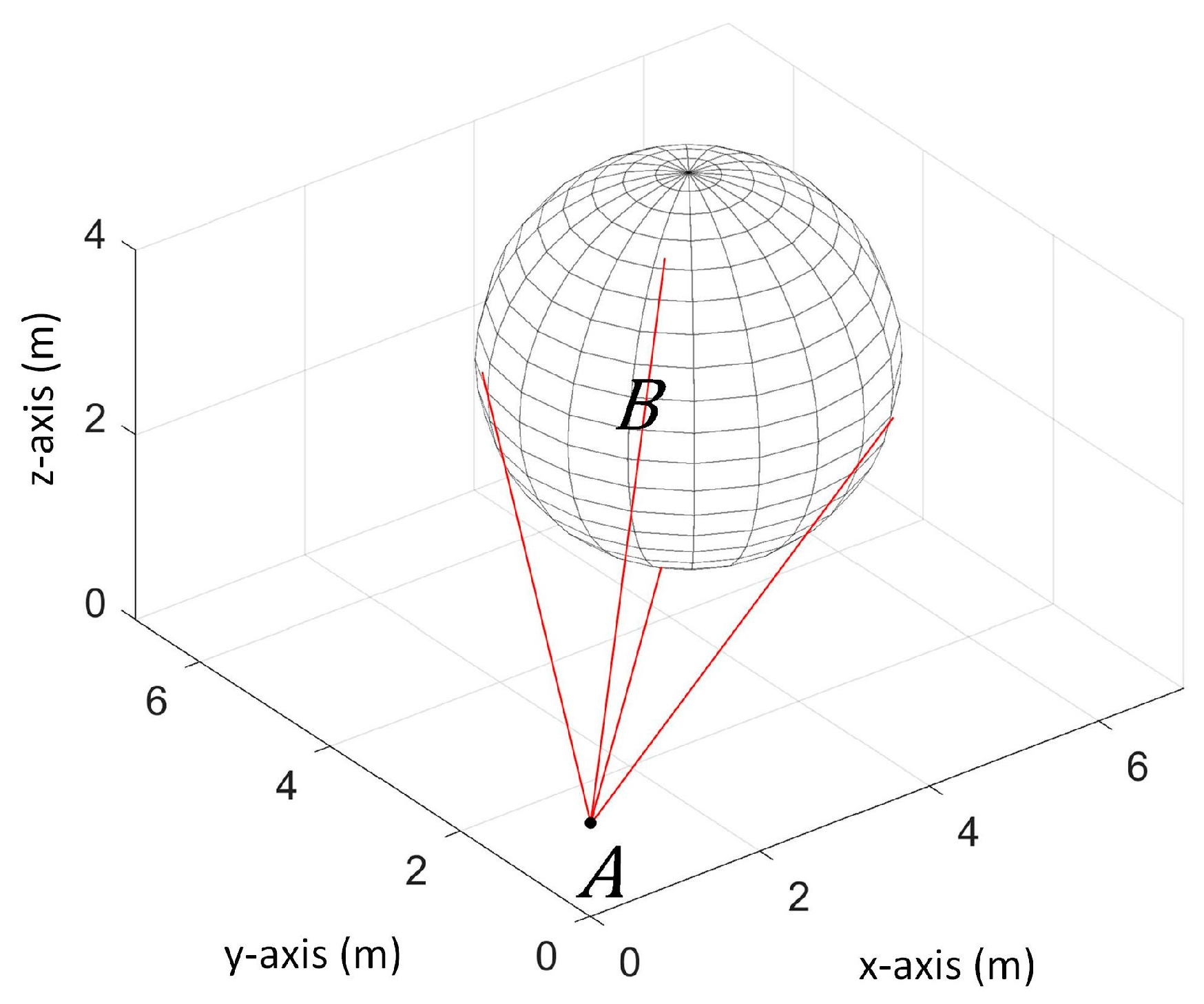
Computing $l{r}_B$

To compute $l{r}_B$, the obstacle should be detected by at least two sensors. In the case that it is detected by only one sensor, this can mean that the obstacle can be very small and therefore we set it to a default $l{r}_B$ value of 0.01 m.

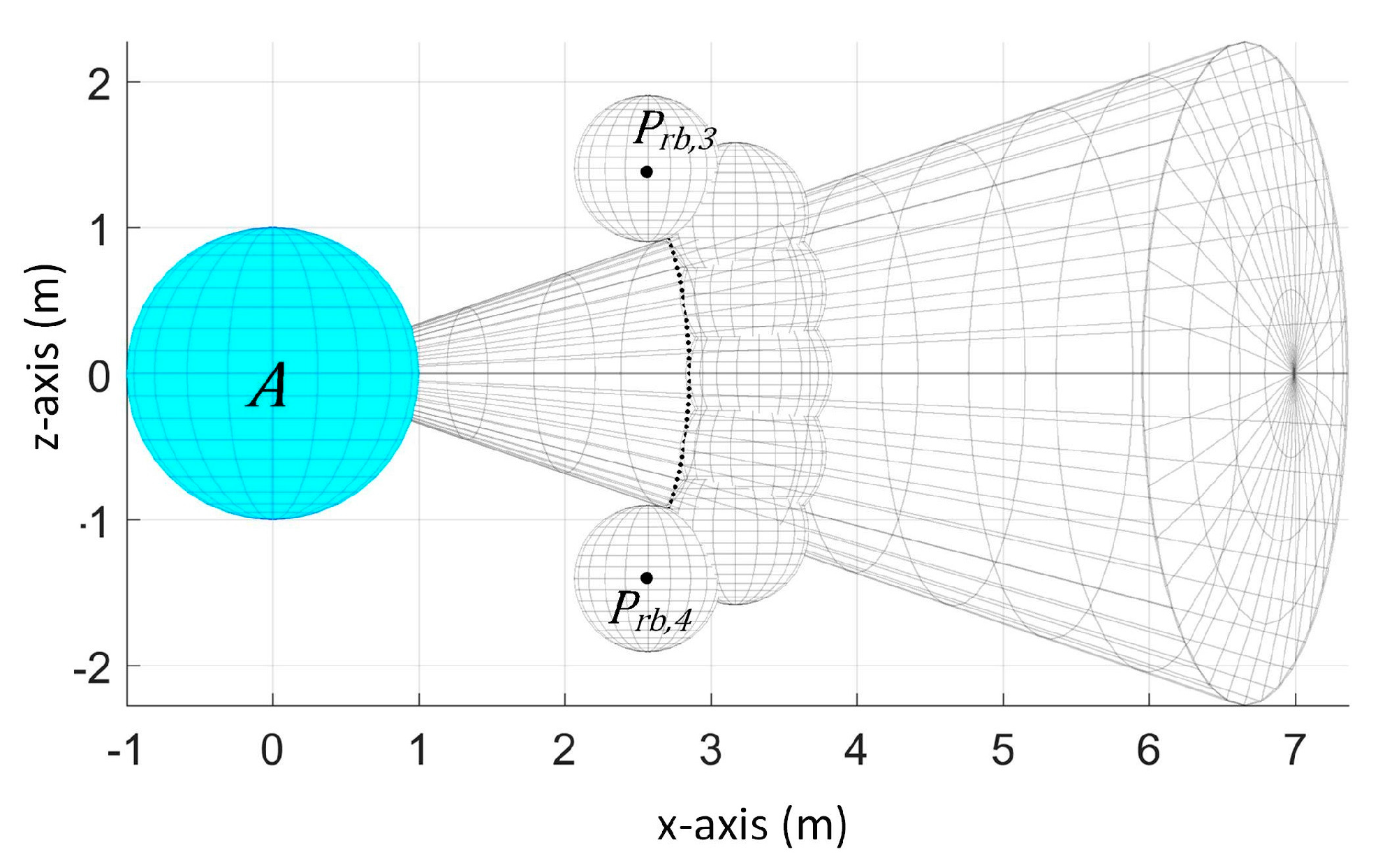
Given at least two sensor readings, let $d_{min}$ be the minimum of $d_s$s and $d_{max}$ be the maximum of $d_s$s. We define the set of points, $P_{\stackrel{\neg }{m}in}$, as the points in the sensing space of the sensor whose reading is $d_{min}$. In other words, every element of set $P_{\stackrel{\neg }{m}in}$ has a distance of $d_{min}$ from the UAV’s center. Now denote $P_{\stackrel{\neg }{m}ax}$ as the set of points in the sensing space of the sensor whose reading is $d_{max}$, and every point in $P_{\stackrel{\neg }{m}ax}$ has a distance of $d_{max}$ from the UAV’s center. Points in $P_{\stackrel{\neg }{m}in}$ and $P_{\stackrel{\neg }{m}ax}$ are the possible points in the sensor’s detection range that are on the obstacle’s surface and nearest to the UAV’s center.

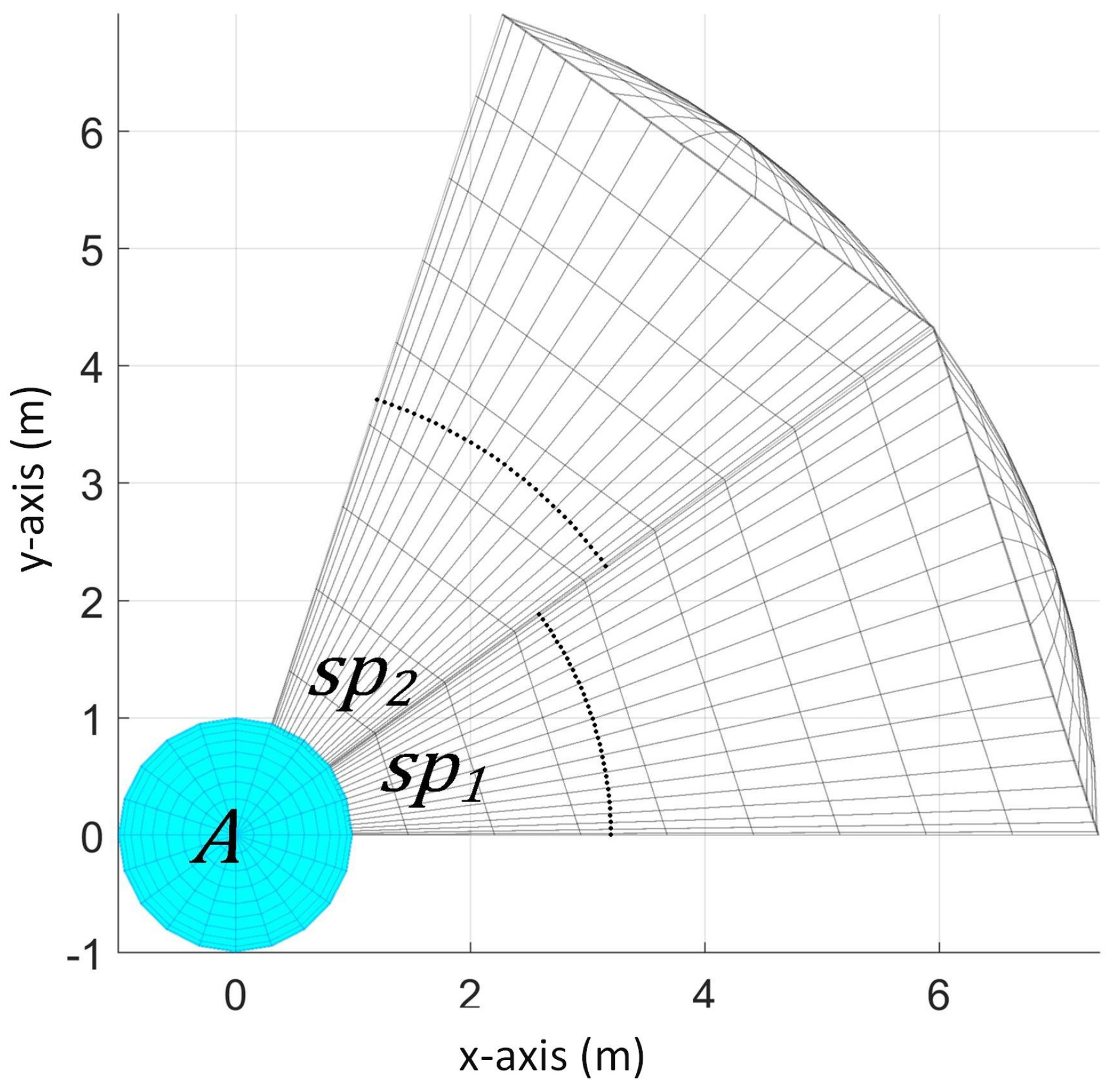
For example, as shown in Figure 7, we have $d_{min}=d_1$ and $d_{max}=d_2$. The points in set $P_{\stackrel{\neg }{m}in}$ are the black points in $s{p}_1$ while $P_{\stackrel{\neg }{m}ax}$ are the black points in $s{p}_2$. From these points, we can get the smallest radius possible if the obstacle is tangent to the boundary of $s{p}_2$ (boundary in the x-y plane thus z = 0 since it is spherical sector shaped) as shown in our example in Figure 8.

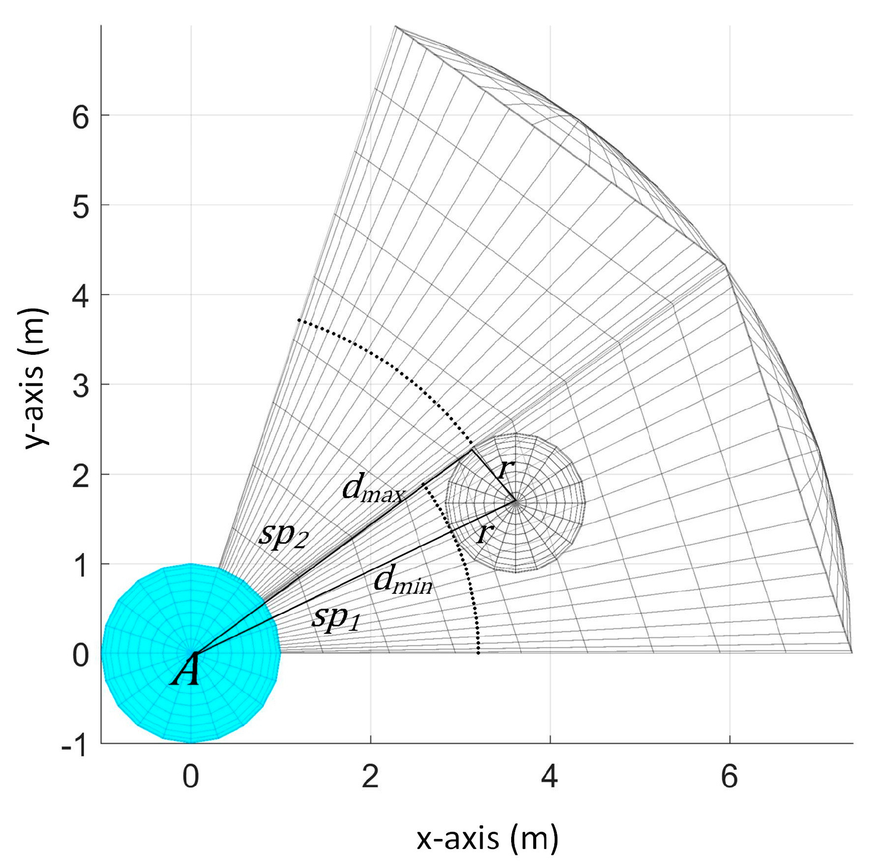
We can get the smallest possible radius of the obstacle using the $d_{min}$ and $d_{max}$, as shown in Figure 9. By applying Pythagorean Theorem, we get the length of the radius $r$ by:

$${\left(d_{min}+r\right)}^2=r^2+d_{max}{}^2$$

(6)

$$d_{min}{}^2+2r{d}_{min}+r^2=r^2+d_{max}{}^2$$

(7)

$$r=\frac{d_{max}{}^2-d_{min}{}^2}{2d_{min}}$$

(8)

$$l{r}_B=\frac{d_{max}{}^2-d_{min}{}^2}{2d_{min}}$$

(9)

5.2. Determining Obstacle’s Possible Positions

We get the possible $p_B$s because the actual $p_B$ cannot be determined given only $d_s$. Aside from $p_B$ as a requirement for $V{O}_{A|B}$, $p_B$ is also needed in our approach to be able to compute the possible $v_B$s. Possible $v_B$ is obtained by getting the difference between possible $p_{B}s$ obtained at current time step and previous time step. Possible $p_B$ is computed based on $d_{min}$ and estimated $r_B$.

In our model, we only know that the obstacle’s center is located in the region of the sensor with $d_{min}$ but we do not know its actual position. Thus, given $d_{min}$ and $r_B$, let us visualize the possible positions of the obstacle’s center. For example, we have $r_B$ and $d_{min}$ where $d_{min}$ is given by sensor 1. As illustrated in Figure 10, looking on the top view (x-y plane), we have the black points to represent $P_{min}$ and the actual center position of the obstacle can be any of the drawn spheres with distances of $r_B$ from the points in $P_{min}$. Note that the possible center positions of the obstacle are not limited to the drawn spheres. We only show limited number of spheres for a clearer illustration. From all these possible center positions, we get the extreme points that lie along the boundary of the sensor’s sensing space denoted as $P_{rb,1}$ and $P_{rb,2}$.

Next, let us look on the side view of the sensing space, which is x-z plane since we consider sensor 1, as illustrated in Figure 11. On this view, we again have the black points to represent $P_{min}$ and the possible center positions of the obstacle are represented by the spheres with distance of $r_B$ from the points in $P_{min}$. Here, the possible center positions of the obstacle can be outside the sensor’s sensing space. We get the extreme points from the possible center points as the highest and lowest possible points in z-axis denoted as $P_{rb,3}$ and $P_{rb,4}$.

We define these considered points as the extreme points since all of the possible center positions of the obstacle are within the region determined by the extreme points. In effect, by considering these extreme points, we can get the maximum possible $v_B$. We are interested in getting the maximum possible $v_B$ so that it is greater than or equal to the actual $v_B$.

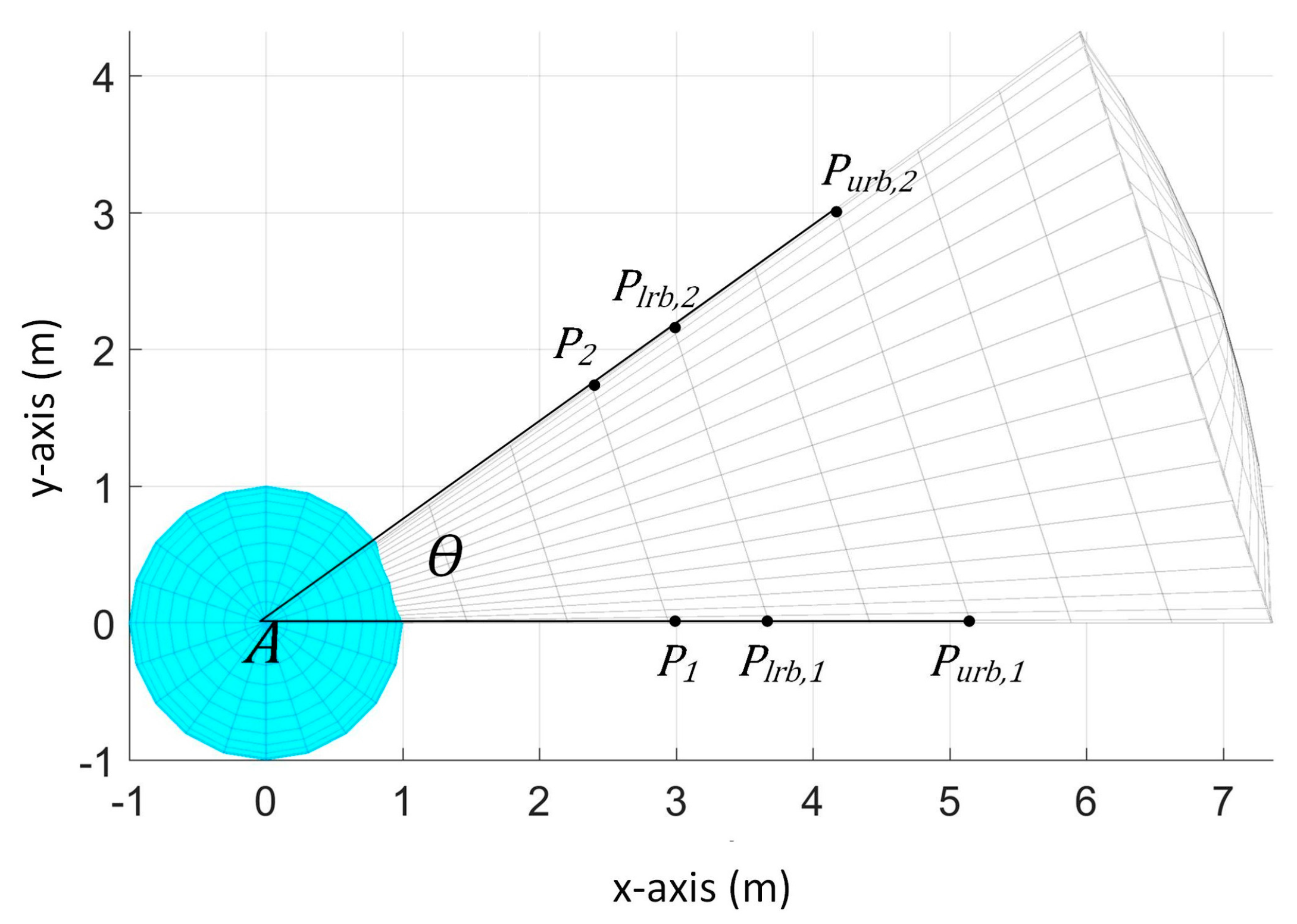
We will now discuss how to compute for the extreme points. First, we show how to compute the extreme points on the border of the sensor’s sensing space in the x-y plane as shown in Figure 12. Since the sensor is spherical sector shaped, the z-coordinate is zero at these borders.

For example, the spherical sector represents the sensing detection space of sensor 1, viewed in x-y plane, with an opening angle of $\theta$. We first get $P_1$ and $P_2$ as points on the border of the sensor with distance of $d_{min}$ from the UAV’s center. Then, we get the point $P_{lrb,1}$ by adding a distance of $l{r}_B$ from $P_1$, and similarly point $P_{urb,1}$ is obtained by adding a distance of $u{r}_B$ from $P_1$. In the same way, we can get $P_{lrb,2}$ and $P_{urb,2}$ by extending $l{r}_B$ and $u{r}_B$, respectively, from $P_2$.

By considering these points, if the obstacle’s center is inside the sensor’s detection range (Case 1), then the actual x and y coordinates of the obstacle’s center is always enclosed in the area surrounded by the points $P_{lrb,1}$, $P_{urb,1}$, $P_{lrb,2}$, and $P_{urb,2}$ since actual $r_B$ is within our estimate of the radius.

Thus, we get the following points:

$$P_{lrb,1}=(\left(d_{min}+l{r}_B\right)\cos (\left(S-1\right)\theta ),\left(d_{min}+l{r}_B\right)\sin \left(\left(S-1\right)\theta \right),0)$$

(10)

$$P_{urb,1}=(\left(d_{min}+u{r}_B\right)\cos (\left(S-1\right)\theta ),\left(d_{min}+u{r}_B\right)\sin \left(\left(S-1\right)\theta \right),0)$$

(11)

$$P_{lrb,2}=(\left(d_{min}+l{r}_B\right)\cos S\theta ,\left(d_{min}+l{r}_B\right)\sin S\theta ,0)$$

(12)

$$P_{urb,2}=(\left(d_{min}+u{r}_B\right)\cos S\theta ,\left(d_{min}+u{r}_B\right)\sin S\theta ,0)$$

(13)

where $S$ is the sensor with $d_{min}$ and $\theta$ is the opening angle of $S$.

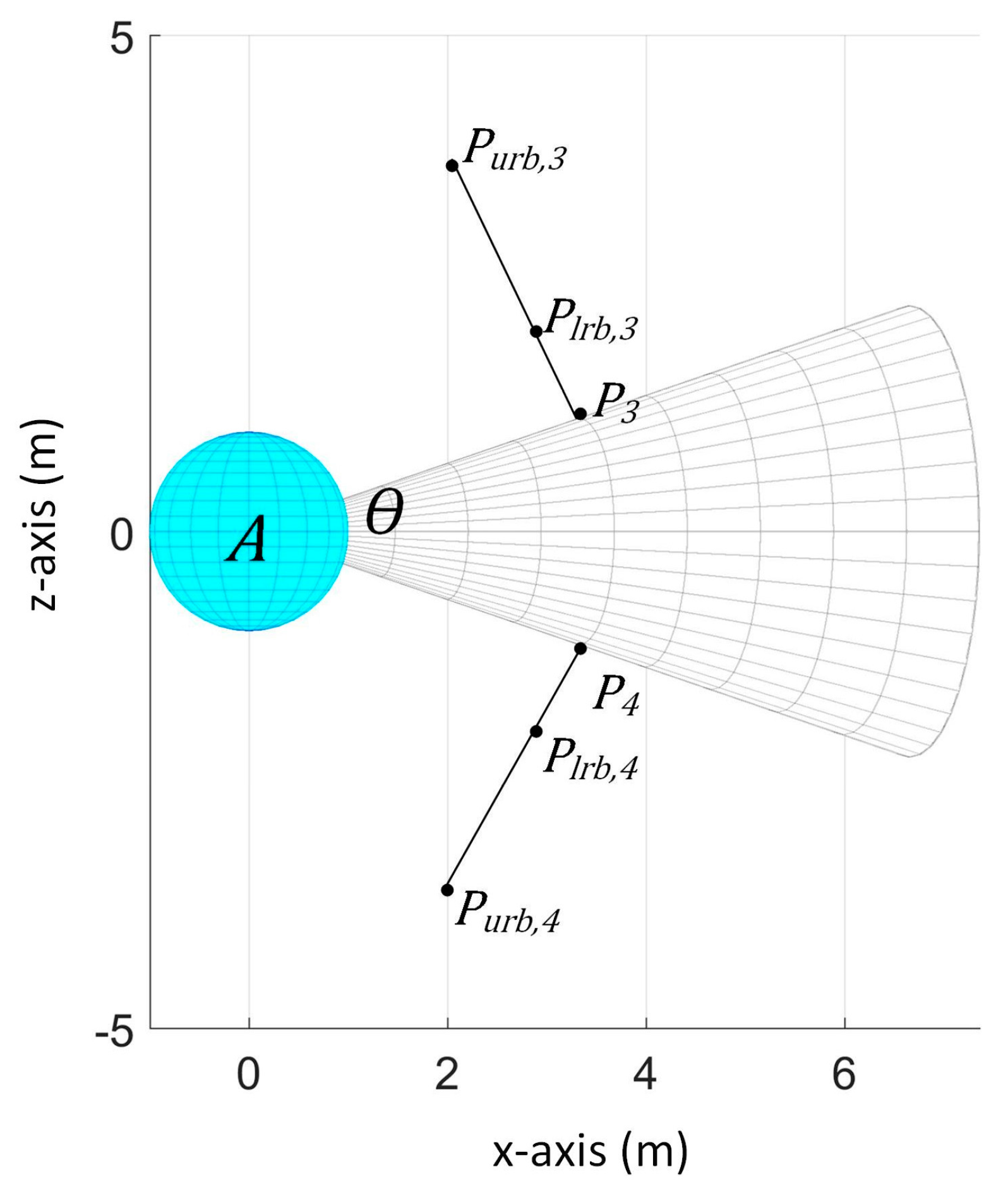
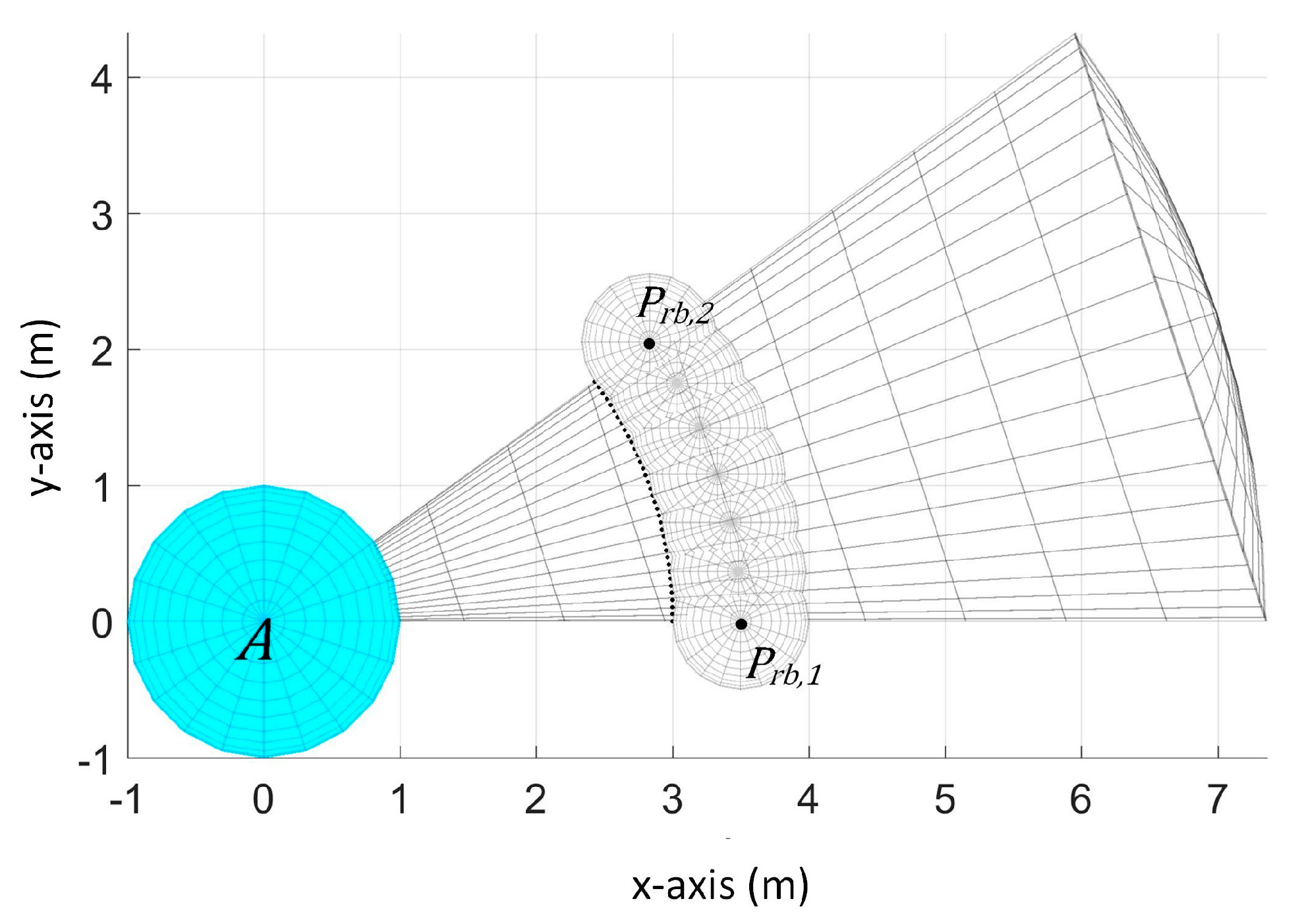
We get the next points to consider the case wherein the obstacle’s center is outside the sensor’s detection range in the y-z or x-z plane (depending on the orientation of the sensor).

For illustration, in Figure 13, sensing space of sensor 1 is viewed in the x-z plane. We denote $P_3$ and $P_4$ as points on the border of the sensing space with distance of $d_{min}$ from the sensor’s vertex. As shown in Figure 13, the highest possible position of the obstacle ($P_{lrb,3}$ with radius $l{r}_B$ and $P_{urb,3}$ with radius $u{r}_B$) is when the obstacle’s center is above the sensing space and the obstacle is tangent to the point $P_3$ and its lowest possible position ($P_{lrb,4}$ with radius $l{r}_B$ and $P_{urb,4}$ with radius $u{r}_B$) is when it is below the sensing space and tangent to the point $P_4$.

We get $P_{lrb,3}$ as the endpoint of a line with length $l{r}_B$ from $P_3$ and the line is perpendicular to the border of the sensing space. In the same way, $P_{urb,3}$ is obtained by creating a line from $P_3$ with length $u{r}_B$. Accordingly, $P_{lrb,4}$ and $P_{urb,4}$ can be obtained by creating lines extending $l{r}_B$ and $u{r}_B$, respectively, from $P_4$.

Thus, we get the following points:

$$P_{lrb,3}=(\left(d_{min}\cos \frac{\theta }{2}-l{r}_B\sin \frac{\theta }{2}\right)\cos \phi ,\left(d_{min}\cos \frac{\theta }{2}-l{r}_B\sin \frac{\theta }{2}\right)\sin \phi ,\left(d_{min}\sin \frac{\theta }{2}+l{r}_B\cos \frac{\theta }{2}\right))$$

(14)

$$P_{urb,3}=(\left(d_{min}\cos \frac{\theta }{2}-u{r}_B\sin \frac{\theta }{2}\right)\cos \phi ,\left(d_{min}\cos \frac{\theta }{2}-u{r}_B\sin \frac{\theta }{2}\right)\sin \phi ,\left(d_{min}\sin \frac{\theta }{2}+u{r}_B\cos \frac{\theta }{2}\right))$$

(15)

$$P_{lrb,4}=(\left(d_{min}\cos \frac{\theta }{2}-l{r}_B\sin \frac{\theta }{2}\right)\cos \phi ,\left(d_{min}\cos \frac{\theta }{2}-l{r}_B\sin \frac{\theta }{2}\right)\sin \phi ,-\left(d_{min}\sin \frac{\theta }{2}+l{r}_B\cos \frac{\theta }{2}\right))$$

(16)

$$P_{urb,4}=(\left(d_{min}\cos \frac{\theta }{2}-u{r}_B\sin \frac{\theta }{2}\right)\cos \phi ,\left(d_{min}\cos \frac{\theta }{2}-u{r}_B\sin \frac{\theta }{2}\right)\sin \phi ,-\left(d_{min}\sin \frac{\theta }{2}+u{r}_B\cos \frac{\theta }{2}\right))$$

(17)

where $\phi =\theta \left(S-\frac{1}{2}\right)$, $S$ is the sensor that gives $d_{min}$, and $\theta$ is the opening angle of $S$.

Since the obstacle’s actual size is within $l{r}_B$ and $u{r}_B$, and we consider the possible $p_B$ in which they are the extreme possible positions using the values of $l{r}_B$ and $u{r}_B$, we can assure that the obstacle’s actual position is enclosed in the surface area formed by the considered points.

We get these points on both the current and previous time step’s sensor readings to be able to determine the change in the location of the points from the previous to current time step which reflects its velocity.

5.3. Determining Obstacle’s Possible Velocities

From the generated possible $p_B$s and time step interval $t_i$, we generate the possible $v_B$s by subtracting previous time step’s generated $p_B$s from current time step’s generated $p_B$s. Since our approach generates values every time an obstacle is detected, it captures the changes in the possible $v_{B}s$ between two consecutive time steps thus it copes with an obstacle with changing velocity.

The set of extreme points obtained using $l{r}_B$ and sensor readings in the current time step is denoted by $P_{lrb}^{tc}=\left\{P_{lrb,1}^{tc},P_{lrb,2}^{tc},P_{lrb,3}^{tc},P_{lrb,4}^{tc}\right\}$ and the set of extreme points obtained using $l{r}_B$ and previous time step’s sensor readings is denoted by $P_{lrb}^{tc-1}=\left\{P_{lrb,1}^{tc-1},P_{lrb,2}^{tc-1},P_{lrb,3}^{tc-1},P_{lrb,4}^{tc-1}\right\}$. Similarly, the set of extreme points obtained from $u{r}_B$ and current time step’s sensor reading is denoted by $P_{urb}^{tc}=\left\{P_{urb,1}^{tc},P_{urb,2}^{tc},P_{urb,3}^{tc},P_{urb,4}^{tc}\right\}$ and the set of extreme points obtained using $u{r}_B$ and previous time step’s sensor readings is denoted by $P_{urb}^{tc-1}=\left\{P_{urb,1}^{tc-1},P_{urb,2}^{tc-1},P_{urb,3}^{tc-1},P_{urb,4}^{tc-1}\right\}$.

We have the generated possible velocities:

$$v_{B,lrB,j,k}=\frac{P_{lrB,j}^{tc}-P_{lrB,k}^{tc-1}}{t_i}\mathrm{for}j,kϵ\left\{1,2,3,4\right\}$$

(18)

$$v_{B,urB,l,m}=\frac{P_{urB,l}^{tc}-P_{urB,m}^{tc-1}}{t_i}\mathrm{for}l,mϵ\left\{1,2,3,4\right\}$$

(19)

Thus, |$v_{B,lrB,j,k}$| = 16 and |$v_{B,urB,l,m}$| = 16.

Again, since our generated possible $p_B$s are the extreme possible center positions of the obstacle, the generated possible velocities will then as a result give the biggest magnitude possible in all directions.

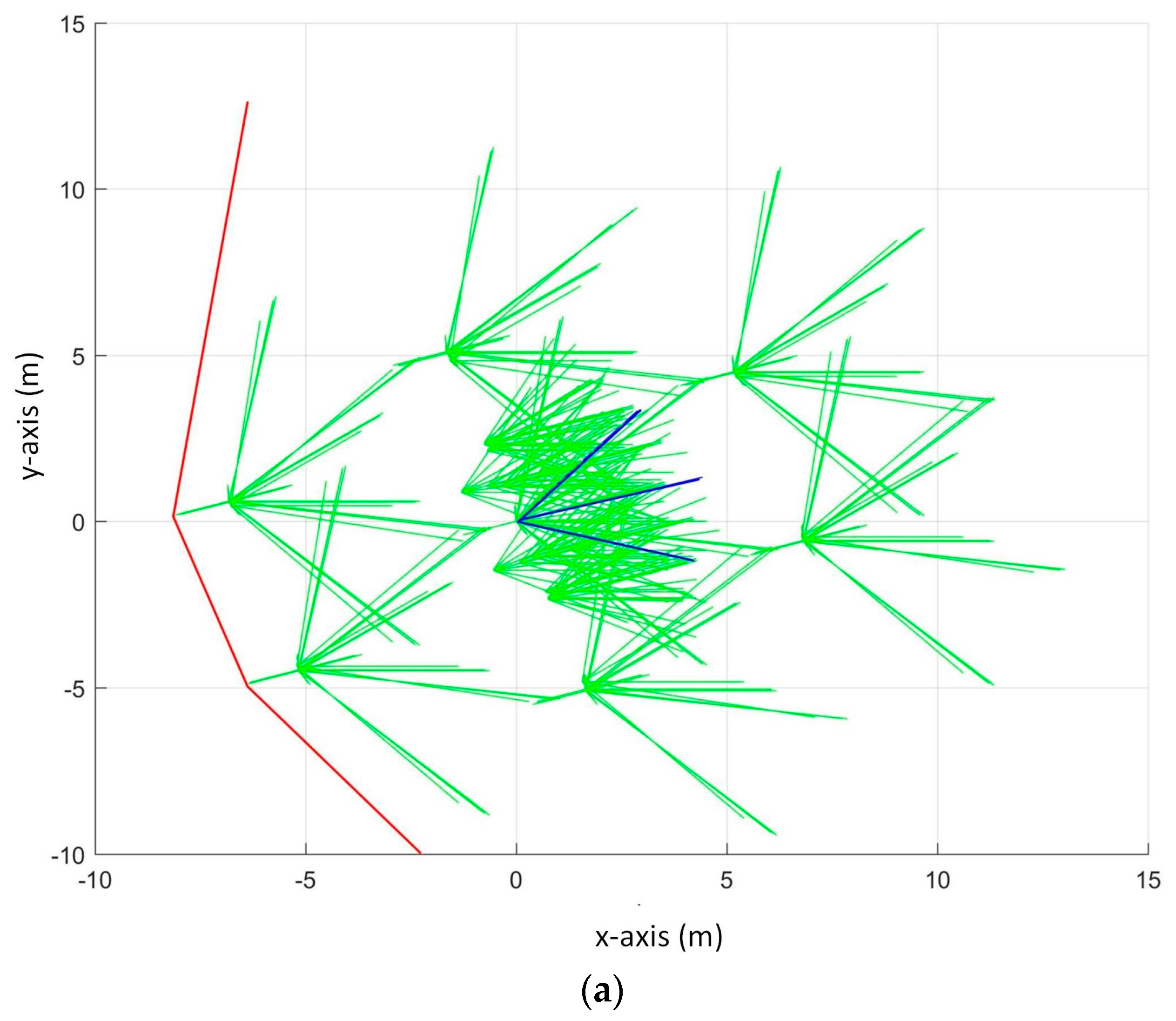
5.4. Generating Possible Velocity Obstacles

Our generated $V{O}_{A|B}$ is constructed from the values of our generated $r_B$, $p_B,$ and $v_B$. The following $V{O}_{A|B}$ is generated for each $t_i$:

$$V{O}_{lrb}\left(P_{lrb,i}^{tc},v_{B,lrB,j,k},l{r}_B\right)\mathrm{for}i,j,kϵ\left\{1,2,3,4\right\}$$

(20)

$$V{O}_{urb}\left(P_{urb,l}^{tc},v_{B,urB,m,n},u{r}_B\right)\mathrm{for}l,m,nϵ\left\{1,2,3,4\right\}$$

(21)

Thus |$V{O}_{lrb}$| = 64, |$V{O}_{urb}$| = 64, and all generated $\left|V{O}_{A|B}\right|=$128.

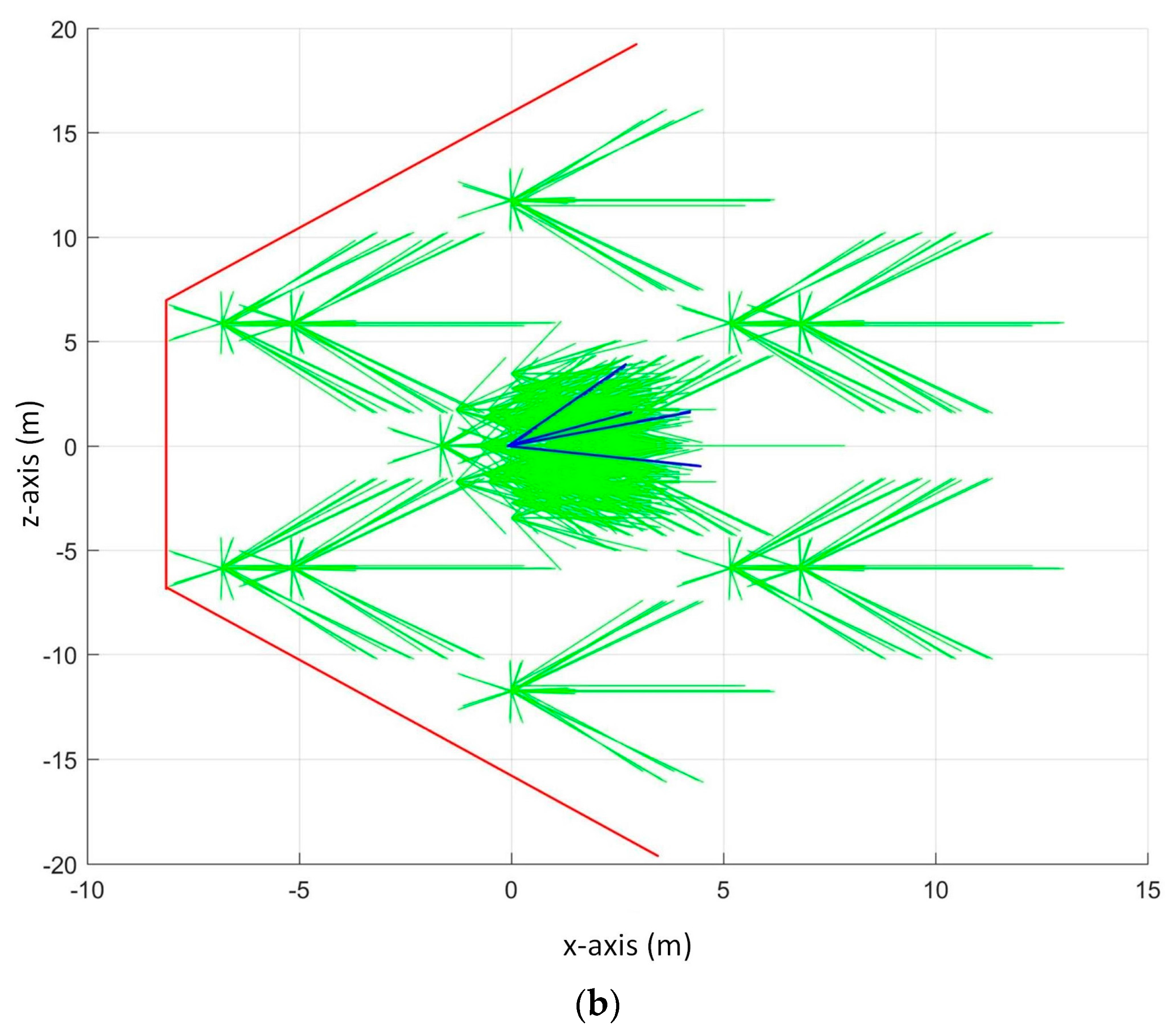
In Figure 14, the blue lines represent the actual $V{O}_{A|B}$, the green lines represent our constructed possible $V{O}_{A|B}$s and the union of the generated possible $V{O}_{A|B}$s is represented by the red lines.

The UAV should choose a velocity outside all of the generated $V{O}_{A|B}$s. Since the actual $V{O}_{A|B}$ is within the union of our generated $V{O}_{A|B}$s, the UAV will choose a velocity that will avoid collision. We can guarantee that the actual $V{O}_{A|B}$ is within our generated $V{O}_{A|B}$s since the obstacle’s actual values are within our generated values.

The following conditions on the UAV’s velocity and goal’s position in relation to the $V{O}_{A|B}$ to guarantee collision avoidance exist:

• The UAV is guaranteed to avoid collision in the next time step given that the UAV’s maximum allowable velocity can reach the velocities outside the generated $V{O}_{A|B}$s. Otherwise, it will stay in its position and may collide with the obstacle in the next time step.
• When the UAV must only choose a velocity towards the goal, it is possible that the UAV cannot reach the goal when the goal is inside the generated $V{O}_{A|B}$ and the obstacle is not moving. On the other hand, when the obstacle is moving away from the UAV, the UAV can wait until there is a possible velocity towards the goal that is outside the generated $V{O}_{A|B}$. Another way wherein the UAV can reach the goal is if it is allowed to travel on a velocity that is moving away from the goal.

6. Collision Avoidance Algorithm

In our algorithm, when no obstacle is detected, the UAV will move at maximum velocity towards the goal. Otherwise, we determine the obstacle’s possible parameter values based on $d_s$. First, we compute the $l{r}_B$ and then we update its value if the new value is greater than the current value. Then, we get the possible $p_B$s if there is a reading from the previous time step. Next, possible $v_B$s are computed from generated $p_B$s then $V{O}_{A|B}$s are created using the generated possible values of $v_B$, $r_B$, and $P^{tc}$. Finally, the UAV chooses a velocity outside that is outside all of the generated $V{O}_{A|B}$s. We repeat this for every time step until the UAV has reached its destination. The pseudocode for this is provided in Algorithm 1.

To find the path to the goal, we use the following heuristics for deciding the velocity that the UAV will take. For both of the heuristics, the UAV must choose a velocity outside all of the generated $V{O}_{A|B}\prime s$.

• To Goal Search (TG): Choose path only towards the goal. The UAV will start to choose path using its maximum speed. However, if the maximum speed is inside the generated $V{O}_{A|B}$, it can choose slower velocity as long as it is towards the goal.
• Maximum Velocity Search (MV): Choose path even if it does not direct towards the goal as long as it is using maximum velocity. In our simulations, we allowed angle deviation up to 180 degrees from the angle of the line connecting the UAV and the goal. Thus, it is possible for the UAV to move backwards when no avoidance maneuver is reachable in its front.

Algorithm 1: Collision Avoidance

assign value to $u{r}_B$ while UAV does not reach goal   if obstacle is detected     compute $l{r}_B$     if there is previous sensor reading       for each possible $r_B\in \left\{l{r}_B,u{r}_B\right\}$         get $P^{tc}$ based on $r_B$         get $P^{tc-1}$ based on $r_B$         get possible $v_B$s using values from $P^{tc}$ and $P^{tc-1}$         for each computed possible $v_B$           Get $V{O}_{A|B}$ using $v_B$, $r_B$, $P^{tc}$         end for       end for       based on heuristic, choose velocity that is outside of all generated $V{O}_{A|B}$s     else UAV stays at position   else UAV moves at maximum velocity towards goal end while

Our algorithm has a constant time complexity, since there are a fixed number of values to be computed for every run. The computation time is about 2 m on a system using Intel Core i7-4790 with 3.60 GHz clock speed. To consider more realistic system that has lower processing power, we developed another version that takes into account the processing delay $\Delta$. When the system has low processing power, then $\Delta$ is significant and must be addressed in the algorithm. In ideal case, when $\Delta =0,$ if the obstacle is detected in $t_i$, the decision can be applied immediately at $t_i$. Otherwise, when $\Delta >0,$ the decision for $t_i$ can be applied only at $t_i+\Delta$ and this causes a problem since the UAV continuously changes position until $t_i+\Delta$ but the decision is made assuming that the UAV’s position is not changed.

To address this, we assign a margin to $\Delta$ that is less than the time step interval. Then, when the decision processing started at $t_i$, the UAV continually moves until $t_i+\Delta$ and the decision on the next velocity is applied to UAV’s position at $t_i+\Delta$. Accordingly, when choosing a velocity for the next time step, we consider the reachable velocities from the UAV’s position at $t_i+\Delta$. The approach to the computation of the obstacle’s information is still the same since we still choose a velocity that will avoid the obstacle at $t_{i+1}$.

Under some special situations, collision avoidance cannot be guaranteed. We describe the situations in detail as follows:

• When the obstacle’s current position is not detectable by any of the sensors and the obstacle’s velocity in the next time step will make it collide with the UAV as shown in Figure 15. In Figure 15, the black arrow represents the obstacle’s velocity and blue arrow represents the UAV’s velocity. In this scenario, the UAV has no chance to plan its avoidance maneuver since it did not detect the obstacle before the collision.
• The UAV stays at its position in the next time step after an obstacle is first detected. On this instance that the UAV is not moving, there will be collision when the time step interval is not enough for the UAV to plan its next velocity. This means that the obstacle has already collided with the UAV even before the UAV has decided on its next velocity.

7. Simulation

The proposed algorithm was tested in simulations. The simulations were performed on different scenarios. Scenarios 1–3 show common moving directions of the obstacle. The obstacle moves forward-leftward in Scenario 1, backward-leftward in Scenario 2, and leftward in Scenario 3. Scenarios 4 and 5 show the worst case scenario wherein the obstacle is between the UAV and the goal and the obstacle is moving towards the UAV. TG and MV heuristics were used in the simulation. For each scenario, we also show results of the algorithm that takes into account $\Delta$ where $\Delta =0.5$ s using MV search. The results when $\Delta =0.5$ s using TG search are not shown since the UAV is not allowed to change its moving direction to the goal in TG search thus the trajectory is not affected by $\Delta$.

The following parameters were constant in the simulation:

• Sensor’s distance range = 7 m. UAV can detect obstacle within 7 m.
• Time step $t_i$ increments at every 1 s. We generate $V{O}_{A|B}$ and choose UAV’s velocity every $t_i$.
• Default $u{r}_B$ = 5 m
• Default $l{r}_B$ = 0.01 m
• UAV’s initial position = (0, 0, 0) unless otherwise stated
• UAV’s radius = 1 m
• Goal’s position = (0, 13, 5) unless otherwise stated

7.1. Scenario 1

For this scenario, the obstacle’s radius is 2 m, initial position at $t_0$ = (6, 4, 2). The obstacle is moving with constant velocity ($v_x$ = −1 m/s, $v_y$ = 1 m/s, $v_z$ = 0 m/s). Figure 16 and Figure 17 show the path taken by UAV in this scenario using TG search and MV search, respectively.

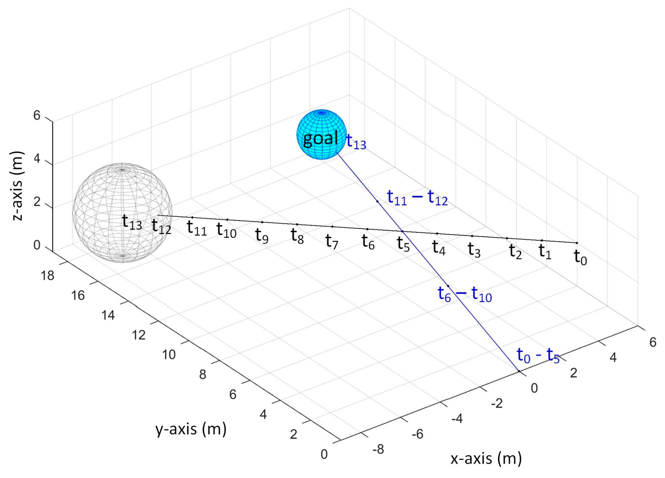
In TG search, the UAV detected the obstacle at $t_0$ and decided to stay at position until $t_4$. It did not detect the obstacle at $t_5$ so it moved towards the obstacle. However, it detected the obstacle again at $t_6$, thus it stopped until $t_9$. It started to move again at $t_{10}$ and detected the obstacle again at $t_{11}$ so it stopped again. At $t_{12}$, no obstacle is detected so it started to move and it finally reached at goal at $t_{13}$.

In MV search, the UAV also stays at position at $t_0$ because it detected the obstacle. Then it moved backward-upward-rightward at $t_1$. It moved backward-upward-leftward at $t_2$ to avoid the obstacle. It moved towards the goal at $t_3$ and $t_4$ because the obstacle is not detected in these time steps. It detected the obstacle at $t_5$ and moved backwards at $t_6$. Then it moved again towards the goal at $t_7.$ The UAV repeatedly moved in this pattern until it reached the goal at $t_{14}$.

When $\Delta =0.5\mathrm{s}$, the UAV continually moves from $t_2$ until $t_2+\Delta$ and the avoidance maneuver for $t_3$ is done at $t_2+\Delta$. It moved towards the goal at $t_3$ and stopped at $t_4$ because the obstacle is detected and then it moved towards right at $t_5$ to avoid the obstacle. The obstacle is not detected at $t_6$ so it moved towards the goal. Then, it moved in forward and backward pattern and reached the goal at $t_{13}$.

7.2. Scenario 2

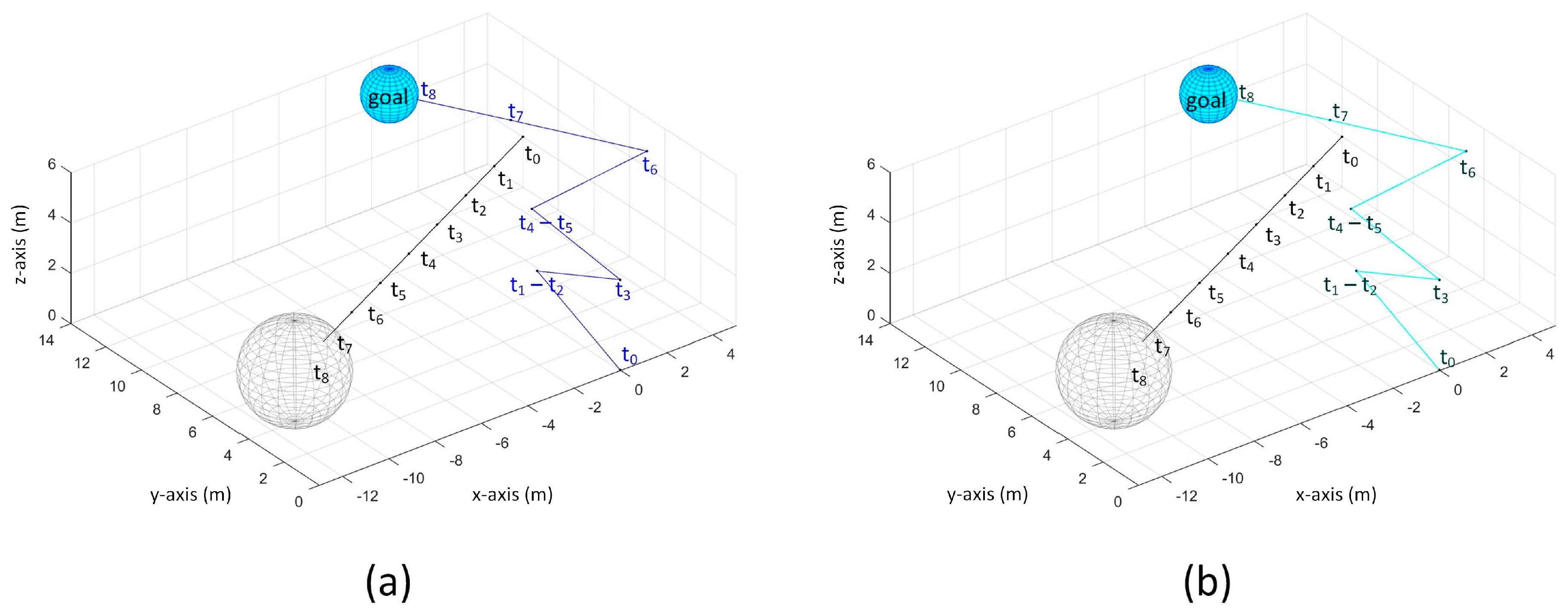
For this scenario, the obstacle’s radius is 2 m, position at $t_0$ = (5, 12, 2). The obstacle is moving with constant velocity ($v_x$ = –2 m/s, $v_y$ = −1 m/s, $v_z$ = 0 m/s). Figure 18 and Figure 19 show the path taken by UAV in this scenario using TG search and MV search, respectively.

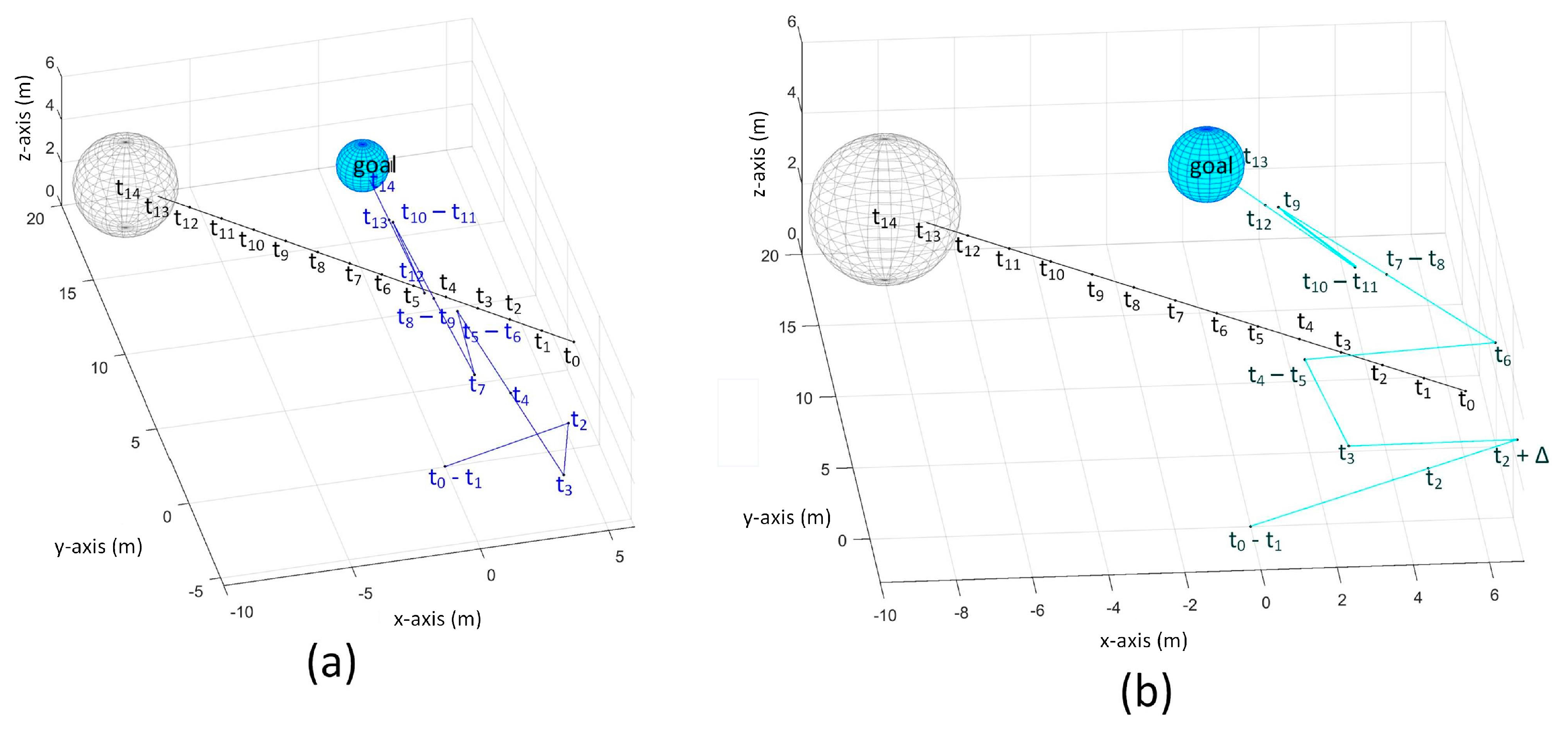
Using TG search, the UAV moved towards goal with maximum velocity at $t_0$ since no obstacle is detected. Then at $t_1$, it detected the obstacle and it stayed at its position until $t_7$. It started to move again towards the goal at $t_7$ and $t_8$ then it reached the goal at $t_9$.

In MV search, the UAV moved towards goal at $t_0$. Then, it stayed at position at $t_1$. It goes backward-upward at $t_2$ to avoid the obstacle. Then it moved forward at $t_3$ because no obstacle is detected and stayed at its position until $t_4$. Then, at $t_5$, it moved backward-rightward. Then starting from $t_6$, it moved towards the goal until it reached the goal at $t_8$. Same trajectory is obtained when $\Delta =0.5\mathrm{s}$ because no time step is affected by the processing delay when the obstacle is not detected in the next time step.

7.3. Scenario 3

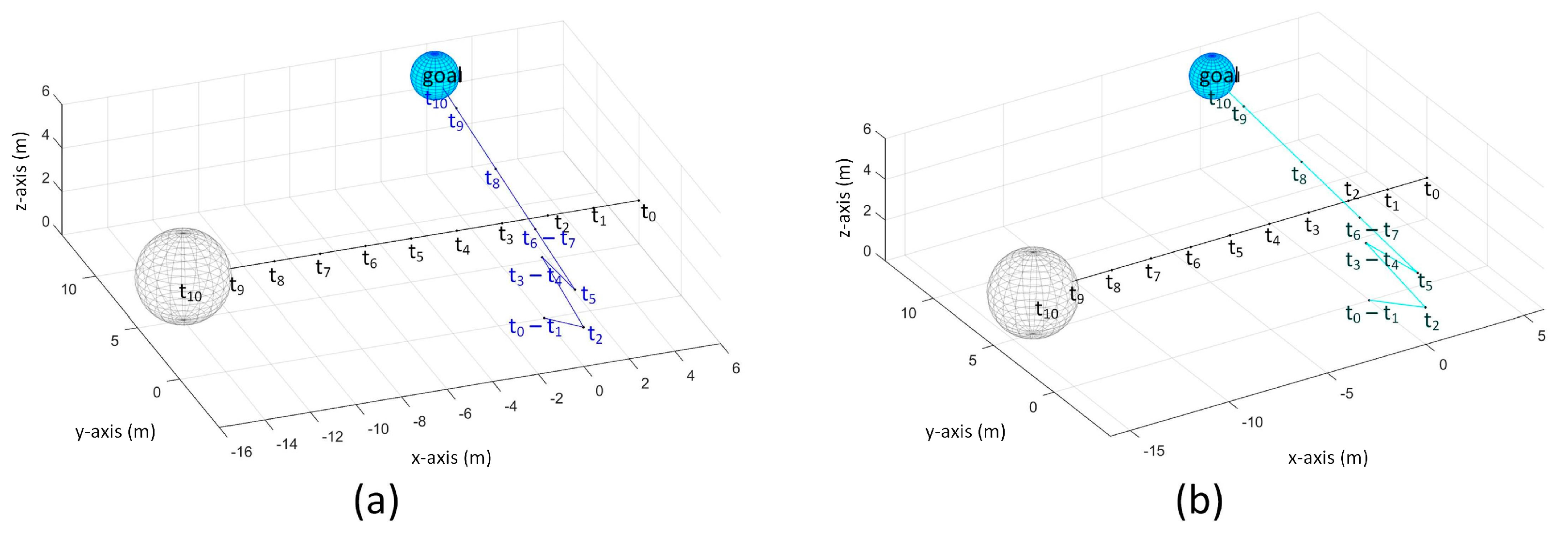
For this scenario, the obstacle’s radius is 2 m, position at $t_0$ = (6, 5, 2). The obstacle is moving with constant velocity ($v_x$ = −2 m/s, $v_y$ = 0 m/s, $v_z$ = 0 m/s). Figure 20 and Figure 21 show the path taken by UAV in this scenario using TG search and MV search, respectively.

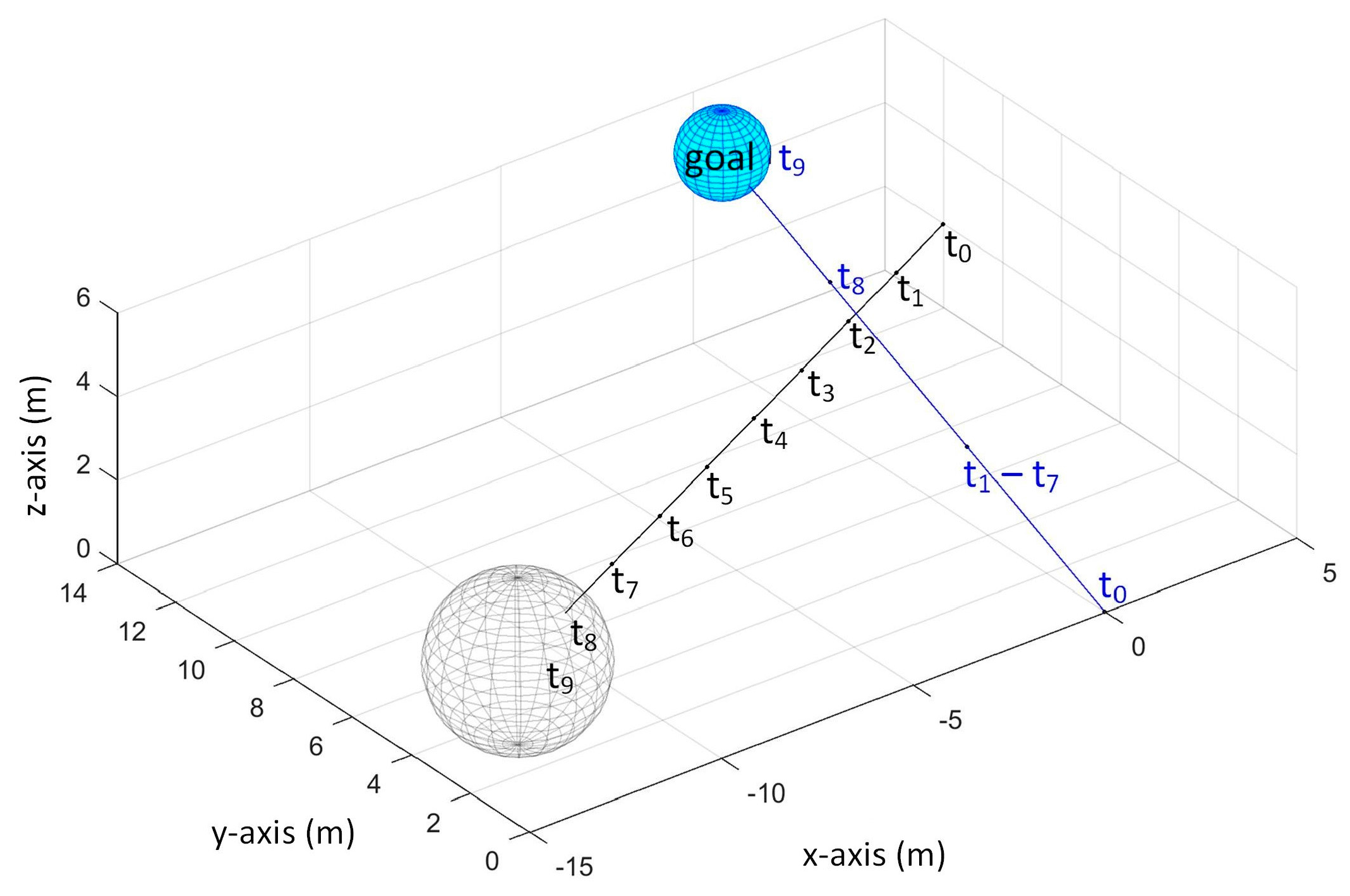
For the TG search, the UAV detected the obstacle at $t_0$ and so it did not move until the obstacle has passed by. After the obstacle has passed by at $t_7$, it moved with maximum velocity. It reached goal at $t_{10}$ (corresponding to 10 s).

In MV search, the UAV detected the obstacle at $t_0$ and so it moved backward-leftward-upward at $t_1$ to avoid the obstacle. It did not detect the obstacle at $t_2$ so it moved towards the goal. However, it detected the obstacle again so it moved backward again at $t_4$. Starting at $t_5$, the obstacle is not detected so it moved straight towards the goal and reached the goal at $t_{10}$. Again, same path is taken when processing delay is considered for this scenario.

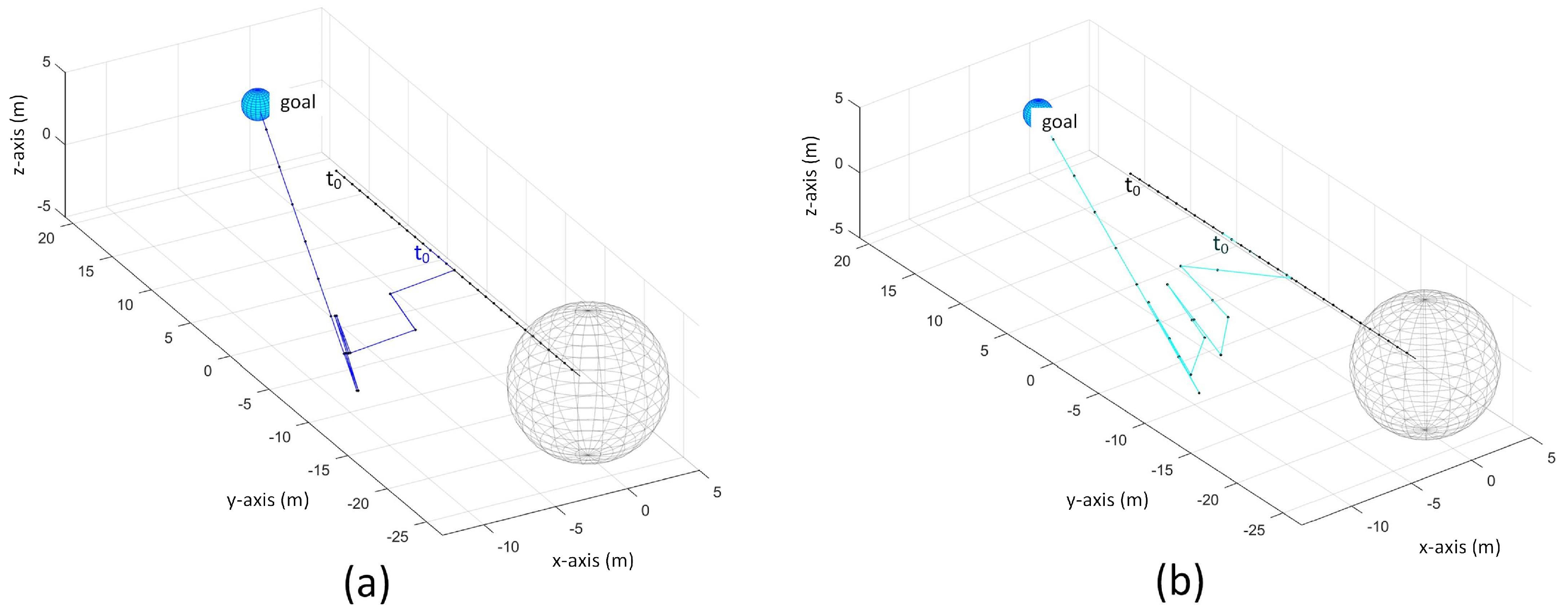
7.4. Worst Case Scenario

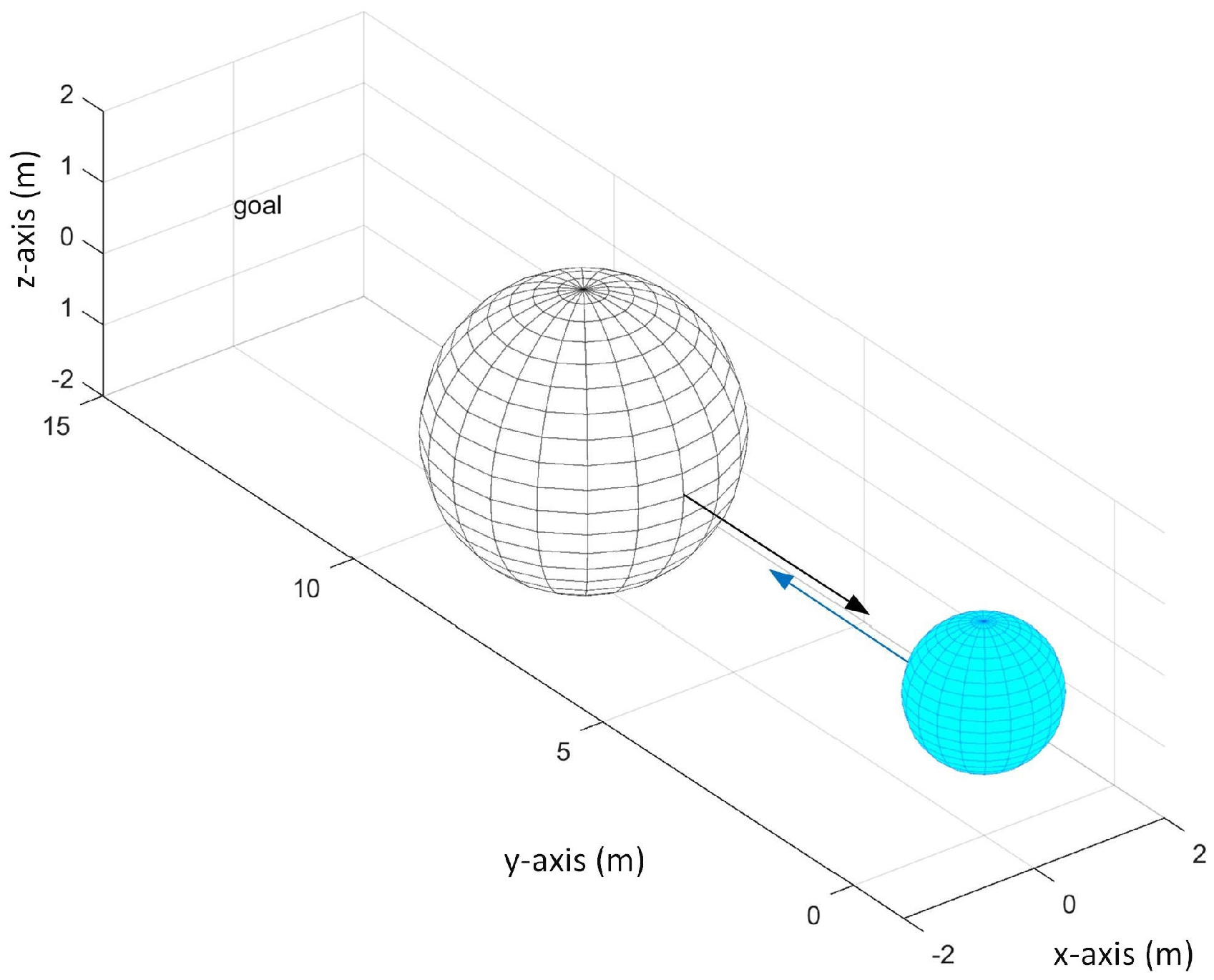
We consider a worst case scenario when the obstacle is located between the UAV and the goal and the obstacle is moving towards the UAV as shown in Figure 22. Obviously, this scenario will not work with TG search so we only show results in MV search.

7.4.1. Scenario 4

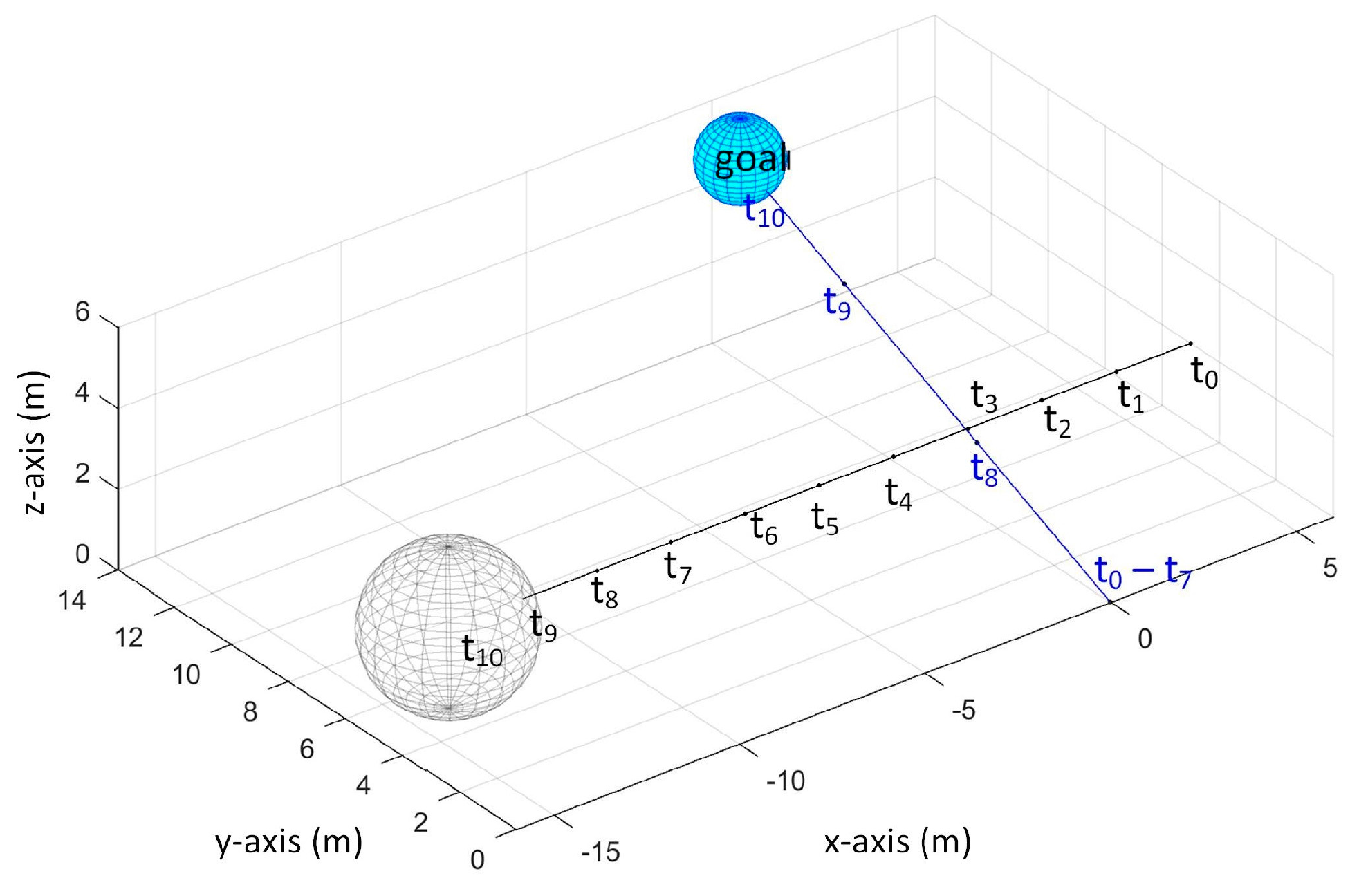
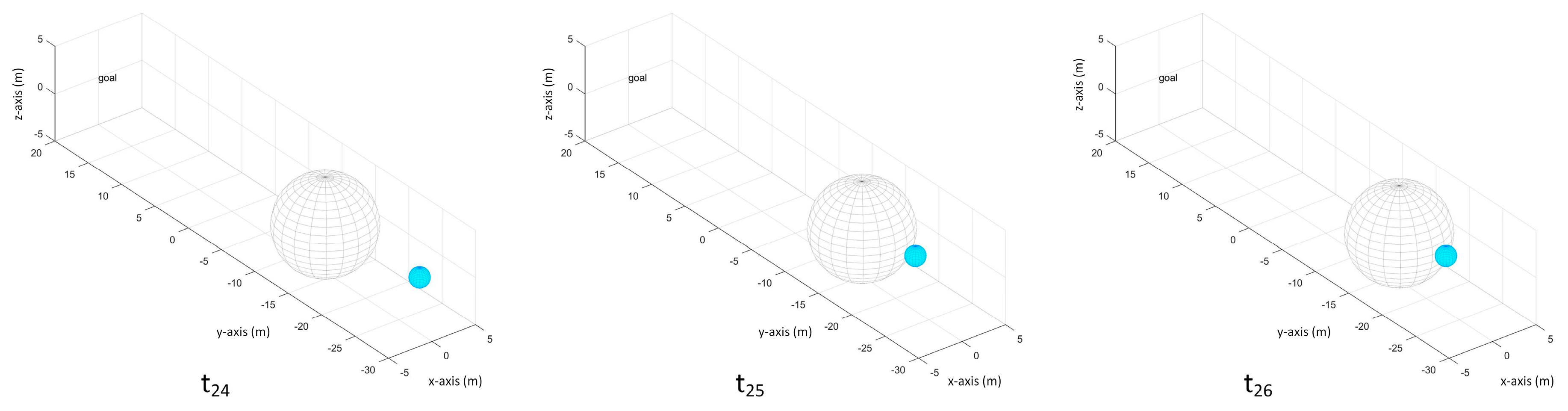
In MV search, we tested it when the obstacle’s position at $t_0$ = (0, 10, 0), goal’s position = (0, 20, 0), UAV’s initial position = (0, 0, 0), obstacle’s velocity ($v_x$ = 0 m/s, $v_y$ = −1 m/s, $v_z$ = 0 m/s), and obstacle’s radius is 5 m. The trajectory of the UAV and the obstacle is shown on Figure 23. In this scenario, the UAV kept on moving backward to avoid the obstacle but it has collided with the obstacle at $t_{26}$. This is because the obstacle is not detected at $t_{24}$ thus the UAV moved forward towards the goal. Then, at $t_{25}$, the obstacle is detected for the first time again so the UAV stayed at its position at $t_{26}$ but the obstacle has collided with the UAV on this time step while the UAV is planning for its next move. The position of the UAV and obstacle at $t_{24}$, $t_{25}$, and $t_{26}$ are shown in Figure 24.

7.4.2. Scenario 5

Another simulation was run with similar parameters in the Scenario 4 but the obstacle’s position at $t_0$ = (0, 15, 0). In this case, the UAV also kept on moving backward similar to the previous simulation but there was no collision and the UAV was able to reach the goal as shown in Figure 25.

Since Scenarios 4 and 5 have different initial position of the obstacle, it resulted to different sensor readings, thus generated different $V{O}_{A|B}$ and provided different choices of the velocities to be taken by the UAV. For this reason, the UAV’s trajectory are different on Scenarios 4 and 5.

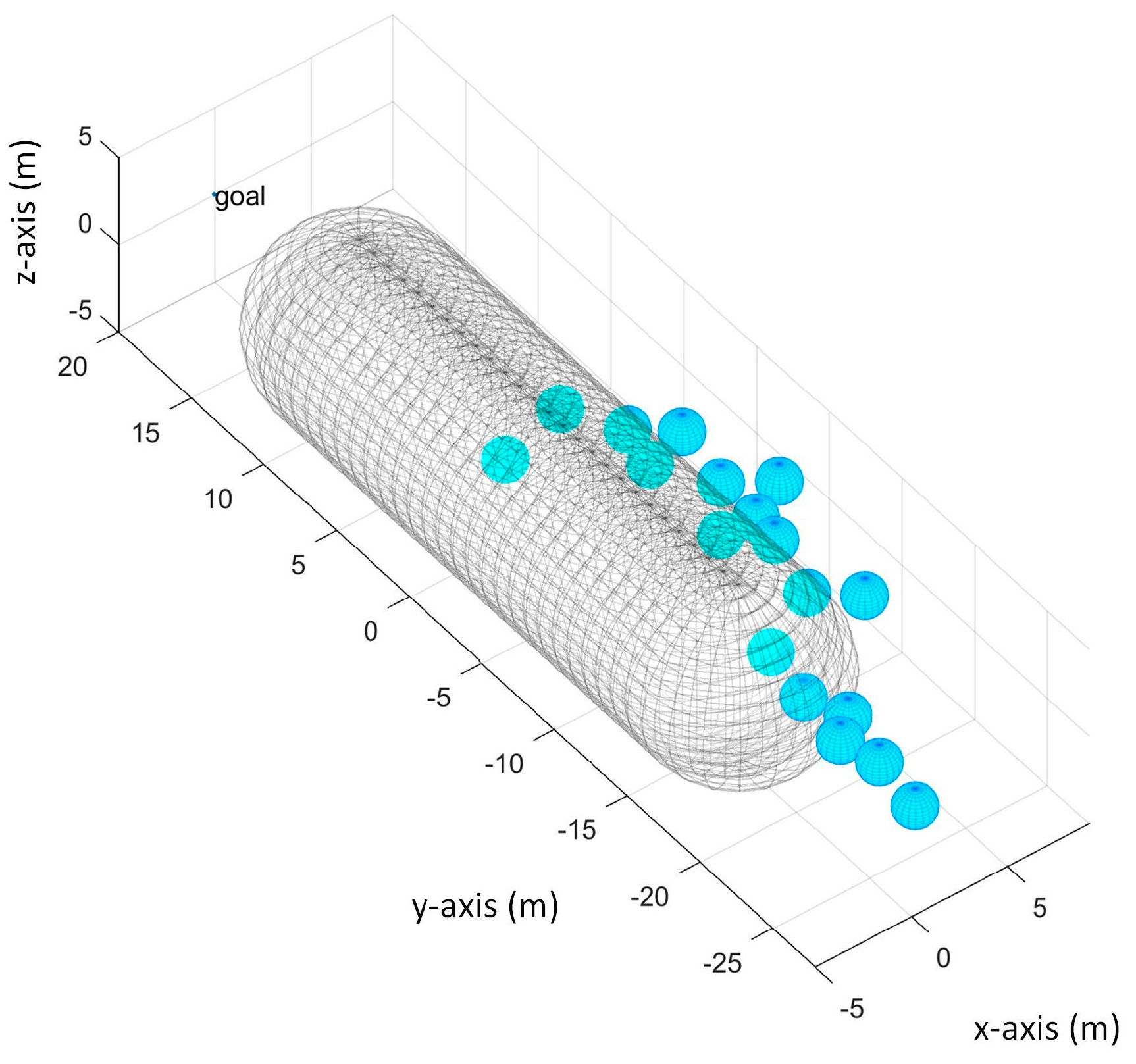
7.5. Velocity Obstacle on Different Obstacle Sizes

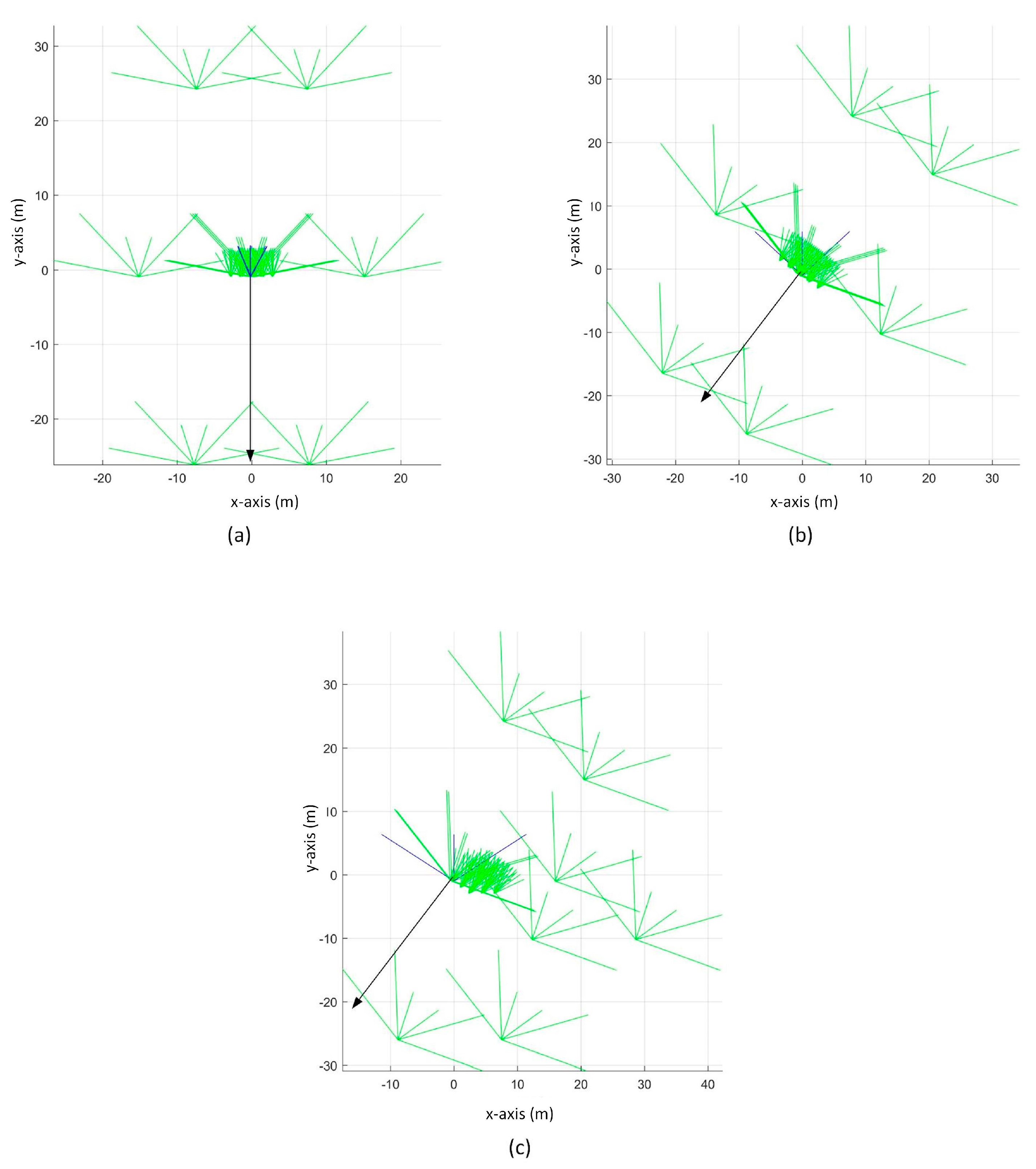
We obtained the velocity obstacles on obstacles with varying obstacle sizes. First, we set $u{r}_B$ = 20 m. Then we examined the generated velocity obstacles when the actual obstacle’s size is 1 m, 10 m, and 20 m. For all of the obstacles, we positioned them at the front of the UAV and made their nearest distances from the UAV similar.

The generated velocity obstacles, represented by the green lines, are shown in Figure 26. The blue lines represent the actual velocity obstacle. Figure 26a shows the velocity obstacle when the obstacle’s size is 1 m, Figure 26b is when the obstacle’s size is 10 m, and Figure 26c is when the obstacle’s size is 20 m. Even though the obstacle’s sizes are different, the covered ranges of their corresponding velocity obstacles do not have big differences.

The black arrow line represents the velocity with shortest distance from the UAV’s center that is outside the generated velocity obstacles. It can be observed that all of the velocities have similar magnitudes which are around 25 m per time step. Thus, for these scenarios, collision avoidance is guaranteed only when the UAV’s velocity allows a magnitude of at least 25 m per time step. This is because the velocity obstacle is generated not based on the actual obstacle’s size but based on the $u{r}_B$ and $l{r}_B$. The bigger value assigned to $u{r}_B$, the bigger scope of the velocity obstacle will be and faster speed of the UAV is needed to be able to guarantee collision avoidance.

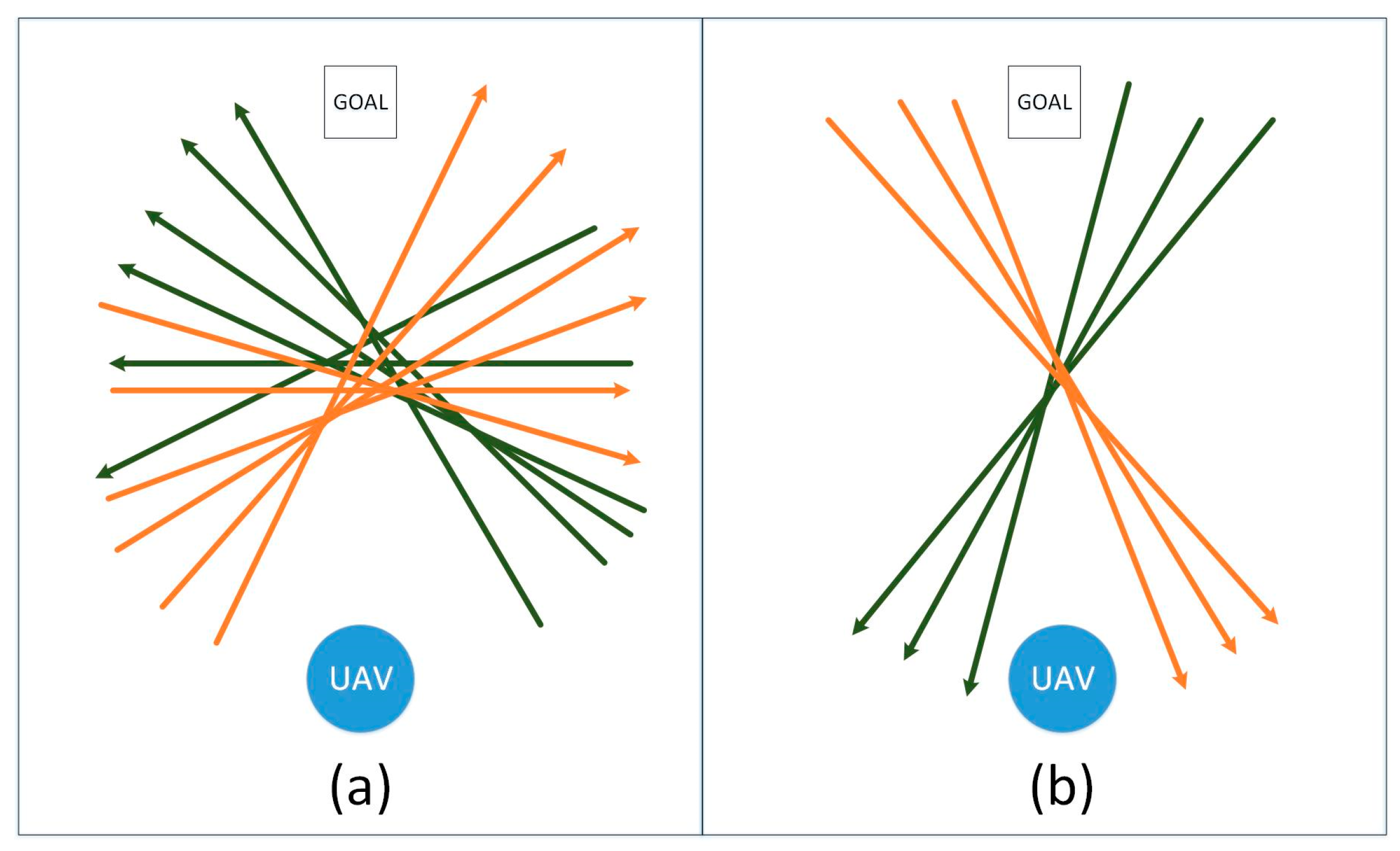
7.6. UAV’s Travelled Distances for Different Obstacle Moving Patterns

More simulations are run using different moving patterns of the obstacle to reflect the appearance of the obstacle in UAV’s detection range at random times. In each simulation, the goal’s position = (0, 20, 0), the obstacle’s radius is 2 m, and obstacle’s speed is in between 0.75 and 2.5 m/s. Figure 27 shows the moving patterns of the obstacles that are used in the simulations. One direction is used for each simulation. In these scenarios, the obstacle is detected by the UAV in random point in time, depending on the obstacle and UAV’s location in each time step. In Figure 27, the arrow lines show the moving patterns of the obstacle, and the circle is the UAV’s initial position. The shortest distance from the UAV’s initial position to the goal is 20 m. The orange lines are the directions to the right while the green lines are to the left.

As observed on the simulations, the effect of the obstacle’s moving pattern to the UAV’s travelling distance can be grouped into two. In the first group, as shown in Figure 27a, the obstacle’s directions mostly move away from the UAV, while it can be seen that, in Figure 27b, the directions move towards and closer to the UAV. These moving patterns in Figure 27b have greater effect on the UAV’s trajectory and the average travelled distance of the UAV for the obstacles’ moving patterns in Figure 27b is 80 m. On the other hand, the average travelled distance of the UAV in Figure 27a is 50 m.

8. Conclusions

We have presented a solution for 3D collision avoidance on a low-cost UAV using the velocity obstacle approach. The UAV’s limited sensing capability limits our knowledge on the environment of the UAV. Because of this limitation, we derived the needed obstacle parameter values to be able to apply the velocity obstacle approach. Finally, from our generated velocity obstacles, we searched for the UAV’s trajectory to the goal using the To Goal (TG) heuristic and Maximum Velocity (MV) heuristic. We also implemented another approach that takes into account the processing delay of the system. We showed our results on scenarios with different obstacle velocities, and different obstacle starting positions. The results also show that our approach works even when processing delay is not negligible. We also showed a special scenario wherein collision happened.

It was also observed that the value assigned to $u{r}_B$ is critical in our algorithm. Greater value assigned to $u{r}_B$ makes the covered range of the generated velocity obstacles bigger and the UAV must be capable of travelling a velocity outside the generated velocity obstacles to guarantee collision avoidance.

In general, using MV search gives more possible avoidance maneuver to the UAV as compared to the TG search in which the velocity is limited to only with direction towards the goal. Hence, in TG, the UAV may decide to stay in its position, while, in MV, the UAV can choose velocity while maintaining the UAV’s maximum allowable velocity. However, in some cases, using MV makes the UAV go farther away from its goal making TG search reach the goal faster.

As mentioned previously, our approach cannot be applied to avoid collisions with multiple obstacles. To make that possible, it is required for the system to have capabilities to identify different obstacles and to track them. Then, more accurate information on the sizes and moving patterns of the obstacles will be available to the system and the proposed method can be applied to avoid collision with multiple obstacles. For this, visual information about the obstacles will be required.

In this study, the focus is on the evaluation of the applicability of the velocity obstacle approach to the collision avoidance scheme of a UAV with limited sensing capability. In the next step, to deal with real flights, the algorithm needs to be tested in a realistic simulation to validate its performance considering the flight dynamics, sensor noise, and external disturbances.