Carbon Footprint Estimation in Fiber Optics Industry: A Case Study of OFS Fitel, LLC

Abstract

Detailed carbon footprinting assignments have been on the rise in more and more major manufacturing industries. The main strength of carbon footprinting is to make product manufacturers aware of carbon emissions and understand its meaning due to perceived global warming effects. Carbon foot-printing through life-cycle assessment in conjunction with greenhouse gas (GHG) accounting is essential for identifying opportunities for environmental efficiencies. Case studies of goods that require more complex production elements have also been increasing, like optical fiber manufacturing. From making ultra-pure glass rods to elongating hot fibers, the whole process involves using a high volume of chemicals and extensive energy. Hence, standard numbers addressing carbon footprinting specifically for fiber optics is helpful for the quantification of greenhouse gas intensity, mitigation of global warming, and adaptation against future climate change scenarios. This paper calculates and helps standardize the emission factor for the production of optical fiber from the scope of gate-to-gate: 4.81 tonnes CO₂eq per million meters of produced fiber (which is 72.92 kg CO₂eq per kg of produced fiber) in order to allow other industries to use this information in their own carbon footprint calculations. Since governmental regulatory agencies have largely failed to confront the risks associated with climate change borne by industries, it is essential for all industries to disclose their emissions in a standardized and comparable form in order to develop standard guidelines for all. This paper provides a practical life-cycle approach, concludes with requirements for further research and evaluation.

1. Introduction

Climate-related change does not just affect portions of our planet but also the assets owned and managed by manufacturers itself. According to the Economics Intelligence Unit 2015 expected losses would more than triple (US$13.8 trillion) should global warming reach 6 °C [1]. The report also indicated that only a few global investors have addressed this risk to date; a modest minority of those investors is even able to quantify the carbon footprint of their own portfolios. Although direct damage of carbon emissions is more localized, indirect impacts can affect the entire global economy. Accordingly, asset managers and investors are facing significant challenges diversifying out of assets affected by climate change. However, lack of greenhouse gas (GHG) information in various industrial sectors and lack of governmental enforcement for reporting GHGs are absolute reasons for not having many forecasting models to estimate the economic cost of future climate change. Researchers are making progress in developing models which will soon be available on a commercial scale throughout the world. Having models have an integrated, consistent framework is essential to predict economic growth, GHG emissions, climate change, and the damaging impacts of climate change on the economy. These should in turn be helpful to inform policymakers/industries in setting emission targets in relation to financial performance. Policymakers all over the world are also making progress. On 22 April 2016, an agreement to mitigate the causes of climate change was signed by over 177 countries, including the two biggest polluters, China and the United States in the Paris Agreement under the United Nations Framework Convention [2].

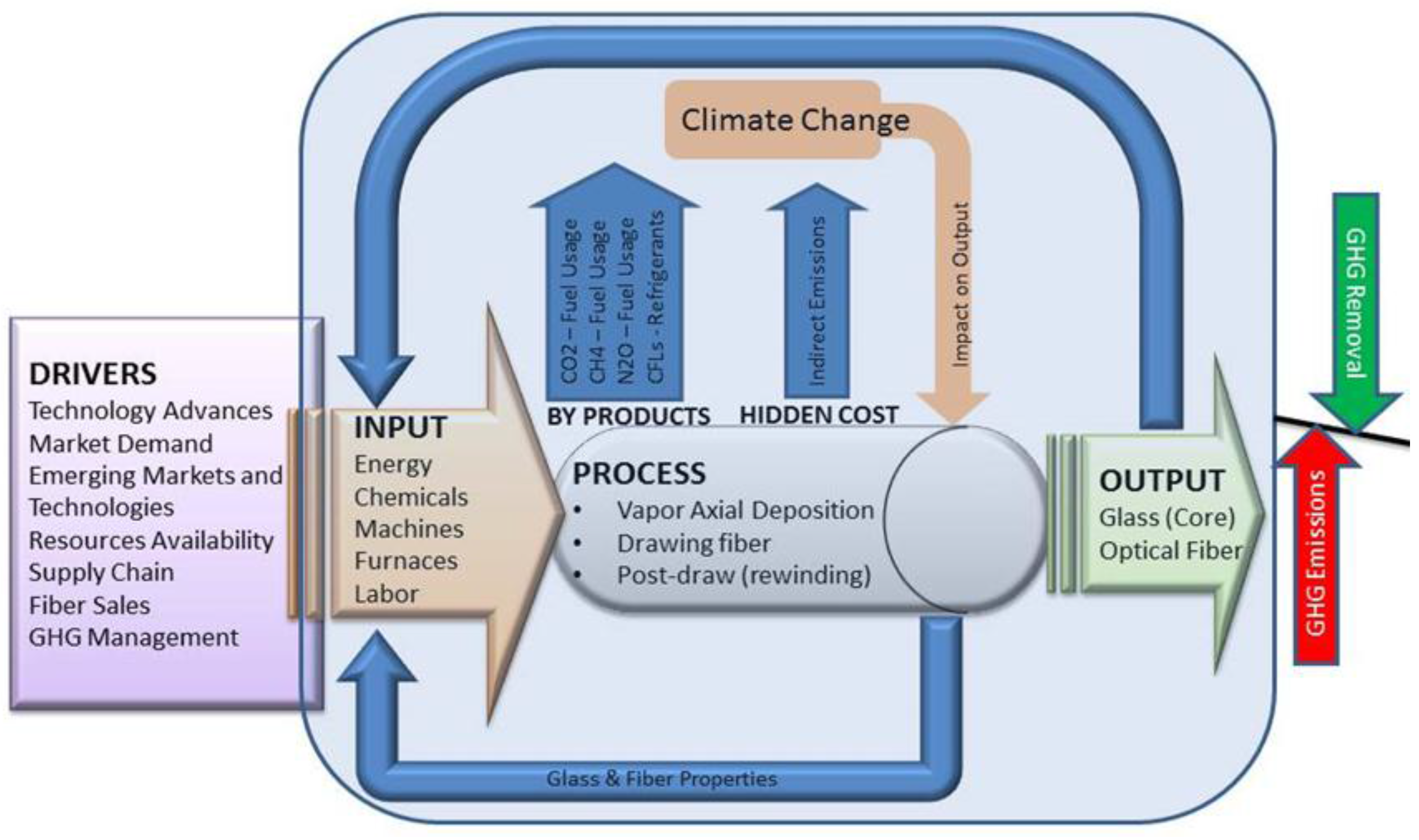
This is why the company Optical Fiber Solutions (OFS) is choosing to spread its GHG knowledge on the optical fiber industry to the public: to try and broaden the knowledge of everyone trying to accurately reflect their own GHG output as culture shifts towards more sustainable practices. The purpose of this case study is to gain insight on the assortment of GHGs in this optical fiber manufacturing company and where they are emitted in the manufacturing process. This case study will also provide an estimation for the current emission factor for optical fiber production, which before this paper, has never been fully and publicly published. Admittedly, this paper only analyzes the emissions from one company, so drawing a general emission factor is a bit difficult. However, OFS currently holds a “World-Leading” market share [3] with its only major competitor being Corning Inc., so using our provided emission factor for optical fiber production is a decent estimation for the full optical fiber market.

OFS will be analyzing its carbon footprint using international standards. A carbon footprint, according to ISO/TS 14067, is the “sum of GHG emissions and removals in a product system, expressed as CO₂ equivalents and based on a life cycle assessment using the single impact category of climate change.” [4] In this case, OFS is looking to calculate the carbon footprint of its optical fiber manufacturing using a gate-to-gate approach, which will be explained later in the Methods section.

The telecommunication industry has a huge potential to reduce its carbon footprint, as 2% of the total carbon footprint of the planet comes directly from running data centers across the world, which uses cables like optical fibers to get the job of data transferring done [5]. In a 2007 economic analysis of the environmental benefits of broadband services, The American Consumer estimated that widespread adoption and use of broadband-based applications could lead to an “incremental reduction of more than 1 billion tons of greenhouse gas emissions (GHGs) over ten years” as it would lead to a greater use of e-commerce, telecommunications, and teleconferencing [6].

General Introduction to the Optical Fiber Industry

Fiber optic technology has many applications leading to tremendous growth in the industry. The applications range from global networks to desktop computers transmitting voice, data, and video information over vast distances in fractions of the time. These feats are accomplished using shockingly few variations in fiber designs. More than just the telecom industry, other large industries utilize these fiber networks, including the oil and gas industry, utilities, private data networks, healthcare/biomedical, among others. Different fibers required for each industry depend on length, cost of installation, and actual application. Specialty fibers have applications in other industries such as the biomedical, automotive, and submarine industries. These markets are wide open for all players and waiting for major innovation breakthroughs.

With reference to the telecommunications industry, TIA TR-42 has initiated a study group for green initiatives in telecommunications infrastructures. The group suggested creating a technical service bulletin (TSB) that includes measures to make telecommunications infrastructures “greener.” For the data center segment within the telecommunications industry, the green metric indicates a reduction in energy consumption and ultimately reduction in CO₂ emissions. The global consortium “Green Grid” is dedicated to improving energy efficiency in data centers and business computing systems all over the world. One of its services is to define metrics for energy efficiency improvements. The “Data Center Energy Productivity (DCeP)” paper publishes a useful metric defined as “useful work produced” by a data center divided by the total energy consumed by a data center [7]. Optical fibers play a significant role in the denominator of the equation when compared to 10 G copper (a very common network cable in data centers today) by reducing network operational and cooling energy.

Data center electrical energy consumption is projected to significantly increase in the next five years. Currently, the biggest data network, the Internet, consumes about 0.4% of the electricity in broadband-enabled countries and the Internet’s energy consumption is expected to increase to 1% as access to broadband increases [8]. A current estimation projects about 14% of CO₂eq from all telecom comes from broadband devices in 2020, up from 3% in 2007 [9]. Solutions to mitigate energy requirements, reduce CO₂ emissions, and support environmental initiatives are being widely adopted. Optical connectivity via optical fibers provides best solution by reduction in power consumption (electronic and cooling) and optimized pathway space utilization necessary to support the movement to greener data centers [10].

2. Methods

2.1. Life-Cycle Approach

The first step in calculating a carbon footprint is to determine the scope of the analysis. The analysis in the following paper uses a life-cycle approach from gate-to-gate. This means that we are concerned about identifying the emissions from the process of manufacturing optical fiber. This will include all burned fuels, all voluntary emissions from scrubbers, all spills, all purchased electricity, and major raw materials’ third-party production emissions. This will not include any third-party transportation costs of the raw materials to OFS, commuting costs of employees, transport costs of final products to where they are sold, or the disposal/recycling of the end-of-life product. Figure 1 is a visual representation of the full cradle-to-grave life-cycle assessment of the optical fiber industry. For the purposes of this case study, the two portions of the process we will worry about are materials processing and fiber production.

2.2. GHG Protocol

To calculate the carbon footprint of any plant, it is important to use standardized methods recognized universally so numbers across industries can be compared to one another. The GHG Protocol lists analytical solutions to calculate the amount of carbon emissions in three sections: Scope 1, Scope 2 and Scope 3. Refer to

Table 1. Definitions for Scope 1, 2 and 3.

Emissions Type	Scope	Definition
Direct emissions	Scope 1	Emissions from operations that are owned and controlled by the company
Indirect emissions	Scope 2	Emissions from the generation of purchased or acquired energy such as electricity, steam, heating or cooling, consumed by the company
Other indirect emissions	Scope 3	Emissions related to downstream transportation and distribution of product

for a simple explanation of Scope 1, Scope 2 and Scope 3.

2.2.1. Scope 1

Scope 1 accounts for the carbon emissions from energy consumption on site, physical and chemical processes, transportation of goods and materials (including people and waste), and any fugitive or excess emissions produced by hardware owned by the plant.

The OFS Norcross Plant operates three (3) natural gas boilers, namely one (1) 40 MMBtu/h Nebraska boiler, one (1) 25.2 MMBtu/h Hurst boiler, and one (1) 9.8 MMBtu/h Bryan boiler. The boilers are used to provide indoor comfort heating by dehumidifying and filtering the humid Georgia air. The manufacturing portions of the plant need the air to be clean and dry because the process of glass manufacturing and fiber manufacturing require a very stable climate (i.e., clean, dry, and temperate). Burning natural gas releases three GHGs: carbon dioxide, methane, and nitrous oxide. To calculate the amount of CO₂-eq emissions, Equation (1) was applied.

$$\begin{array}{ll}{\mathrm{CO}}_2\text{eq from combusting natural gas per year}& =\frac{\text{Volume of combusted natural gas}}{\text{year}}\\ & \times \text{Higher Heating Value of natural gas}\\ & \times \left[\text{Default Emission Factor }\right(\text{EF})\text{ of }{\mathrm{CO}}_2\\ & \times \text{Global Warming Potential }\left(\text{GWP}\right)\text{ of }{\mathrm{CO}}_2+\text{Default EF of }{\mathrm{CH}}_4\\ & \times \text{GWP of }{\mathrm{CH}}_4+\text{Default EF of }{\mathrm{N}}_2\mathrm{O}\times \text{GWP of }{\mathrm{N}}_2\mathrm{O}]\end{array}$$

(1)

All of the constants used in this equation can be found in 40CFR98 (Mandatory Greenhouse Gas Reporting) in Tables A-1, C-1 and C-2 [11]. OFS also uses Distillate Fuel Oil No. 2 as an emergency fuel to power both the emergency generators and the boilers. Fuel oil also emits the three GHGs carbon dioxide, methane, and nitrous oxide, so Equation (1) applies to finding the emission rate for fuel oil as well; the constants just need to be changed to reflect that fuel oil is being burned rather than natural gas. These constants are provided in the same tables as the natural gas constants.

The next requirement is to calculate physical or chemical processes used directly in manufacturing that release GHG emissions. The manufacturing process in the Norcross Plant that emits greenhouse gases into the atmosphere also uses a scrubbing process. Scrubbers filter the emissions of all the different machines at OFS and take out about 70–99% of the harmful chemicals, then expel the residual into the atmosphere. According to internal OFS calculations, a few tons of carbon dioxide, the only GHG released by the scrubbers, is emitted into the atmosphere per year through the scrubbers as a consequence of having the chemical tetrafluoromethane (TFM) being scrubbed. Internal OFS calculations assume a mass balance of 1 mole of CO₂eq emitted per mole of TFM used in the scrubbing process multiplied by the efficiency of the scrubber, which in the case of TFM is 80%.

Any transportation vehicles that are owned by OFS and releases CO₂ emissions needs to be included into Scope 1 calculations. However, OFS currently does not own any transportation vehicles like cars, trains, or planes, so this section is not applicable.

Finally there are fugitive emissions. These are any other emissions released by the plant not mentioned anywhere else in Scope 1. OFS has three general fugitive emissions: General Volatile Organic Carbons (VOCs) from coating and inks, acetone, isopropyl alcohol (IPA) from wipes, and refrigerants from the A/C Units. To calculate the carbon emissions from the general VOCs and IPA, OFS took the amount of general VOCs and IPA present in percentages and multiplied it by three and one half respectively, as this is a good estimate for the global warming potential (GWP) for each. The refrigerant used by the OFS heating/ventilation/air-conditioning (HVAC) system is R-134a. Therefore, using the amount of refrigerant leaked multiplied by the GWP of R-134a gives the amount of CO₂eq leaked by the A/C system at OFS.

All of these results are itemized and shown in the Results section in

Table 2. Using the methods discussed in the previous section and the numbers provided below, these results were obtained for Scope 1.

Type	Compound	Year	Amount	Emission Value [Metric Tons CO2eq]
FUEL	Natural Gas (ft3/year)	2013	113,192,000	6168.49
		2014	105,838,000	5767.72
		2015	97,983,000	5339.66
		2016	106,849,000	5822.82
	Distillate Fuel Oil No. 2 (gallons/year)	2013	-	-
		2014	-	-
		2015	533	5.459
		2016	341	3.492
SCRUBBER	Tetrafluromethane (m3/year)	2013	602.739	1.4203
		2014	788.767	1.8586
		2015	1145.451	2.6991
		2016	1279.646	3.0153
FUGATIVE	General VOCs (metric tons/year)	2013	--	17.70
		2014	--	19.17
		2015	--	18.43
		2016	--	8.05
	Acetone (metric tons/year)	2013	--	-
		2014	--	3.42
		2015	--	3.12
		2016	--	2.24
	A/C Unit (lbs/year)	2013	1950.00	1264.84
		2014	550.00	356.75
		2015	-	-
		2016	-	-
	Scope 1 Emissions (metric tons/year)	2013	--	7452.43
		2014	--	6148.92
		2015	--	5369.37
		2016	--	5839.62

.

2.2.2. Scope 2

Scope 2 emissions, in the case of OFS, consist solely of the emissions caused by purchased electricity. Three GHG compounds are emitted as a result of electricity generation: carbon dioxide, methane, and nitrous oxide. Equation (2) can be used to find the equivalent carbon dioxide emissions for each GHG compound, and those values can be added together for a total result of the amount of carbon emissions caused by purchased electricity. All Scope 2 calculations were done using a calculation tool provided by the GHG Protocol to calculate the CO₂eq of purchased electricity, as illustrated in the Results section in

Table 3. Using the methods discussed in the previous section, these results were obtained for Scope 2.

Greenhouse Gas (GHG)	Emission Factor (kg GHG/kWh)	Global Warming Potential (GWP)	Year	Amount of Electricity Used (kWh)	Emission Value (Amount × Emission Factor × GWP) (kg CO2eq)
Carbon Dioxide	0.614	1	2013	105,763,000	64,938,482.00
			2014	109,119,000	66,999,066.00
			2015	115,121,000	70,684,294.00
			2016	116,762,000	71,691,868.00
Methane	1.04 × 10−5	25	2013	105,763,000	27,366.18
			2014	109,119,000	28,234.54
			2015	115,121,000	29,787.56
			2016	116,762,000	30,358.12
Nitrous Oxide	9.47 × 10−6	298	2013	105,763,000	298,595.60
			2014	109,119,000	308,070.43
			2015	115,121,000	325,015.59
			2016	116,762,000	329,509.37
Scope 2 Emissions	--	--	2013	--	65,264,443.78
			2014	--	67,335,370.98
			2015	--	71,039,097.15
			2016		72,051,735.49

[12].

$$\begin{array}{ll}{\mathrm{CO}}_2\text{eq from purchased electricity}& =\text{Amount of electricity purchased }\left[\mathrm{kWh}\right]\\ & \times \text{EF of substance }\left[\raisebox{1ex}{$\text{kg substance emitted}$}\!\left/ \!\raisebox{-1ex}{$\mathrm{kWh}$}\right.\right]\\ & \times \text{GWP of substance }\left[\raisebox{1ex}{$\mathrm{kg}{\mathrm{CO}}_2\mathrm{eq}$}\!\left/ \!\raisebox{-1ex}{$\text{kg substance emitted}$}\right.\right]\end{array}$$

(2)

2.2.3. Scope 3

This will be a pseudo-Scope 3 analysis because this information will be used later in the results and because the scope of this life-cycle assessment is only from gate-to-gate. To find the emissions caused by purchased goods, one only needs to turn to emission factors. All of the major raw materials used in the production of the product need to be identified, and then multiplied by the emission factor of the respected raw material. An emission factor is usually represented as a unit of CO₂eq emissions per unit of product produced. Therefore, the result will be the amount of carbon emissions it took to make the amount of a raw material used in manufacturing the final product. Equation (3) shows the summation of all raw materials emission values. These results are illustrated in the Results section in

Table 4. Using the methods discussed in the previous section, these results were obtained for Scope 3. This table and the rest of this paper have redacted the names of the company’s raw materials for confidentiality purposes.

Compound	Emission Factor (kg CO2e/kg Raw Material)	Year	Amount Used in Production (kg Raw Material)	Emission Value (Amount × Emission Factor) (kg CO2eq)
Aluminum Sulfate	0.5	2013	135,291	67,645.50
		2014	131,534	65,767.00
		2015	155,797	77,898.50
		2016	121,983	60,991.50
Raw Material A
Raw Material B
Magnesium Sulfate	0.3	2013	77,609	23,282.70
		2014	70,964	21,289.20
		2015	66,973	20,091.90
		2016	71,123	21,336.90
Raw Material C
Sodium Hydroxide	1.12	2013	1,059,209	1,186,314.08
		2014	1,063,892	1,191,559.04
		2015	1,251,471	1,401,647.52
		2016	1,288,417	1,443,027.04
Scope 3 Emissions	--	2013	--	1,277,242.28 + (A, B, C)
		2014	--	1,278,615.24 + (A, B, C)
		2015	--	1,499,637.92 + (A, B, C)
		2016		1,525,355.44 + (A, B, C)

.

$$\begin{array}{ll}{\mathrm{CO}}_2\mathrm{eq}\mathrm{from}\mathrm{purchased}\mathrm{goods}& ={\displaystyle {\displaystyle \sum }_{\mathrm{i}=0}^{\#\mathrm{raw}\mathrm{materials}}}(\mathrm{Amount}\mathrm{of}\mathrm{raw}\mathrm{material}\mathrm{used}\mathrm{in}\mathrm{production}\\ & \times \mathrm{Emission}\mathrm{factor}\mathrm{of}\mathrm{the}\mathrm{raw}\mathrm{material})\end{array}$$

(3)

2.2.4. Emission Factor

After Scope 1, 2 and 3 emissions are calculated, an emission factor will be calculated by dividing the total emissions (Scope 1 + Scope 2 + Scope 3) over the total production of optical fiber. For privacy purposes, the production numbers of OFS will not be recorded in this research paper, but an emission factor for optical fiber will be provided for other industry members who would like to use it for the GHG assessment of their company.

2.3. A Description of the Optical Fiber Industry in OFS

OFS’ facility, located in Norcross, Georgia, currently manufactures single-mode optical fibers. Optical fiber is composed of ultra-high purity glass drawn down to a diameter equivalent to that of a single human hair. This ultra-high purity glass medium allows light to freely pass through it without being distorted. This makes optical fiber ideal for many different applications where the clean transmission of data is critically important. Figure 2 illustrates the optical fiber manufacturing process from a carbon foot-printing perspective. The following is a brief description of how optical fiber is manufactured.

This facility is broken into three main production areas consisting of glass making, draw and post draw. Product flow through the facility is such that all processing is complete once it leaves a specific production area, on its way to final packaging and shipping to the customer.

2.3.1. Glass Making-Production of Preforms

The manufacturing of an optical fiber typically starts with the fabrication of preforms. There are a variety of methods that can be used to fabricate preforms such as Vapor-Phase Axial Deposition (VAD), Outside Vapor Deposition (OVD), or Chemical Vapor Deposition (CVD). In each glass making production area, one or more of these techniques is used to make the solid core glass of the optical fiber. When the optical fiber is in service most of the light travels through this core. The core is further processed to add outer layers of high purity glass cladding to form a large solid cylinder known as a preform. A completed preform is then transported to the draw production area. Figure 3 shows a detailed illustration of a VAD machine and labels important components of the machine.

The main building where production of preforms takes place must be air conditioned with highly purified dry air. This takes up a lot of energy to the point where the filtering and dehumidifying units are powered by burning natural gas. This burning of natural gas is where ~90% of Scope 1 emissions are from. Gaseous outputs of this process are sent to the scrubber, and those gases emitted by the scrubber contribute a small portion to Scope 1 emissions.

2.3.2. Fiber Draw

In the draw production area each preform is heated using furnaces. The preform is placed in the furnace on the top floor of the Draw machine and gravity draws the glass into the very thin fiber. Additional processing in this area includes application of a protective coating to each fiber and each strand of fiber is wound onto a spool for transport to the post draw production area. The manufactured optical fiber consists of the actual fused-silica fiber and the plastic coating, applied during the drawing process. Figure 4 details the components and parts of a draw tower.

This portion of the plant uses many high energy electrical furnaces to heat up the preforms for the draw process. The electrical furnace usage accounts for 80–90% of the electrical usage of the whole plant. All of this electricity comes either from purchased electricity, which would be in the case of OFS Scope 2 emissions, or generated from emergency diesel fuel oil generators, which would be Scope 1 emissions.

2.3.3. Post-Draw

Once on the post draw production area the fiber is processed according to a customer’s specifications. The Rewind Line is also used for repackaging fiber to meet customer orders. It can take stock fiber from inventory and produce different length packages; change spools; color code the fiber; test the strength; and correct or remove some defects. When a customer’s order leaves the post draw production area it is boxed and ready for shipment to the customer. Figure 5 is an illustration of the inside workings of the post-draw machine.

The post-draw, similar to the draw process, draws a large amount of its energy from electrical power. Approximately 10–20% of the total electrical use in this plant is from post-draw. As with draw, the post-draw electricity comes directly from purchased electricity or from emergency diesel fuel oil generators.

3. Results

The carbon footprint of optical fiber products from OFS was quantified and general emission factors were calculated. In addition, hotspots across the life cycle of optical fiber products were identified.

Table 2 shows the results of calculating Scope 1 emissions using the method explained in the “Methods” section. All emission factors used in these results are acquired from 40CFR98 Code of Federal Regulations of the United States, which derive its emission factors from international standards [11]. As can be seen by the results, the boilers are the most significant portion of the carbon footprint for the direct emissions of the plant, and this number has gone down from 2013 to 2015 with a slight uptick in 2016. Another thing to note is the air-conditioning (AC) Unit, when applicable, also contributes a large portion of the Scope 1 emissions. Additionally, it is important to consider any non-operational releases such as material spills as these can be significant contributors. The data below shows the impact of such a spill of the AC Unit’s refrigerant R134a, a highly potent GHG, into the atmosphere, which is why the 2013 and 2014 numbers are higher than expected. Entries in the fuel oil and AC Units in the Emission Value and Amount column are blank as there were no recorded values to put in those spots for that year. The values of General VOCs and Acetone in the Amount column are blank as their emission are directly equal to metric tons of CO₂eq, so there is no need for an intermediary step in which the amounts units change.

Table 3 shows the results of calculating Scope 2 emissions using the method explained in the “Methods” section. These results were computed using the general method in the Methods and the purchased electricity emission factors are directly from the GHG Protocol [12]. This is by far the largest contribution to the carbon footprint in a gate-to-gate scope. OFS uses approximately 100 million kilowatt-hours of electricity each year. For reference, an average American house only uses about 11,000 kilowatt-hours of electricity each year [15]. The amount of electricity used by OFS has gone up by about 10 million kilowatt-hours from 2013 to 2016, increasing the carbon footprint of the plant. This increase in energy usage is closely correlated to the increased production of optical fiber from 2013 to 2016.

Table 4 shows the calculated results of Scope 3 emissions using the method explained in the “Methods” section. Section 3.1 in this report discusses where the emission factors in this table came from and the difficulties with reporting this section. Raw Materials A, B, and C were omitted from this table for security and privacy reasons. These values are indeed used in the final emission factor calculation, but their values will not be provided in this paper. While this section is the lowest of the three, an interesting point is raised regarding the interpretation of these results. From 2013 to 2016, production of optical fiber increased at OFS, therefore, more raw materials are required to make more fiber. This resulted in the Scope 3 emissions rising from 2013 to 2016. However, the true test of how well OFS is stabilizing its carbon footprint is to look at the specific GHGs and total emission factors for optical fiber in

Table 5. Percent change in production and specific GHG emissions of optical fiber products with each production year.

Production Year	Scope	Amount of CO2eq Emitted in Tonnes	Percent Change of Production Compared to OFS_2013	Percent Change of Specific GHG Compared to OFS_2013	Emission Factor for Optical Fiber (Tonnes CO2eq/Million Meters of Fiber)	Emission Factor for Optical Fiber (kg CO2eq/kg of Fiber)
OFS_2013	1	7458.03	--	--	6.60	100.05
	2	65,256.57
	3	1277.242 + (A, B, C)
OFS_2014	1	6154.07	29.52%	−21.69%	5.17	78.35
	2	67,349.46
	3	1278.615 + (A, B, C)
OFS_2015	1	5390.35	46.59%	−27.80%	4.77	72.23
	2	71,030.53
	3	1499.638 + (A, B, C)
OFS_2016	1	5839.62	47.81%	−27.11%	4.81	72.92
	2	72,051.74
	3	1525.355 + (A, B, C)

.

Table 5 shows percent change in production of fiber, percent change of calculated specific GHG emissions, and emission factors for optical fiber production. The values for the percent changes are blank in 2013 as this value was used as the base value and all subsequent percentage are based from that 2013 number. From 2013 to 2016, the specific GHG emissions of optical fiber at this plant have decreased by about 27% and production has increased by 48%. These results show that OFS is using less carbon emissions over the past few years to make more products, which is good from both an environmental and economic standpoint. The emission factor for the production of optical fiber at OFS, in consequence, has decreased, meaning that less CO₂eq is emitted for the production of each fiber. The units for the emission factor are metric tons of CO₂eq per million meters of fiber produced or kilograms of CO₂eq per kilogram of fiber produced.

Table 6. Contributions of the raw materials and the manufacturing stage to the carbon footprint in terms of percentages.

Product	Raw Materials Stage (%)	Manufacturing Stage (%)
OFS_2013	4	96
OFS_2014	5	95
OFS_2015	5	95
OFS_2016	5	95

illustrates how the amounts of the raw materials carbon footprint compare with that of the manufacturing stage. As illustrated, the manufacturing stage makes up about 95% of the carbon footprint in comparison to the roughly 5% attributable to the raw materials’ stage. Most of this table is affected by Scope 2, which accounts for about 90% of the total footprint. Without Scope 2, the relationship between Scope 1 and Scope 3 would be about 60:40 respectively.

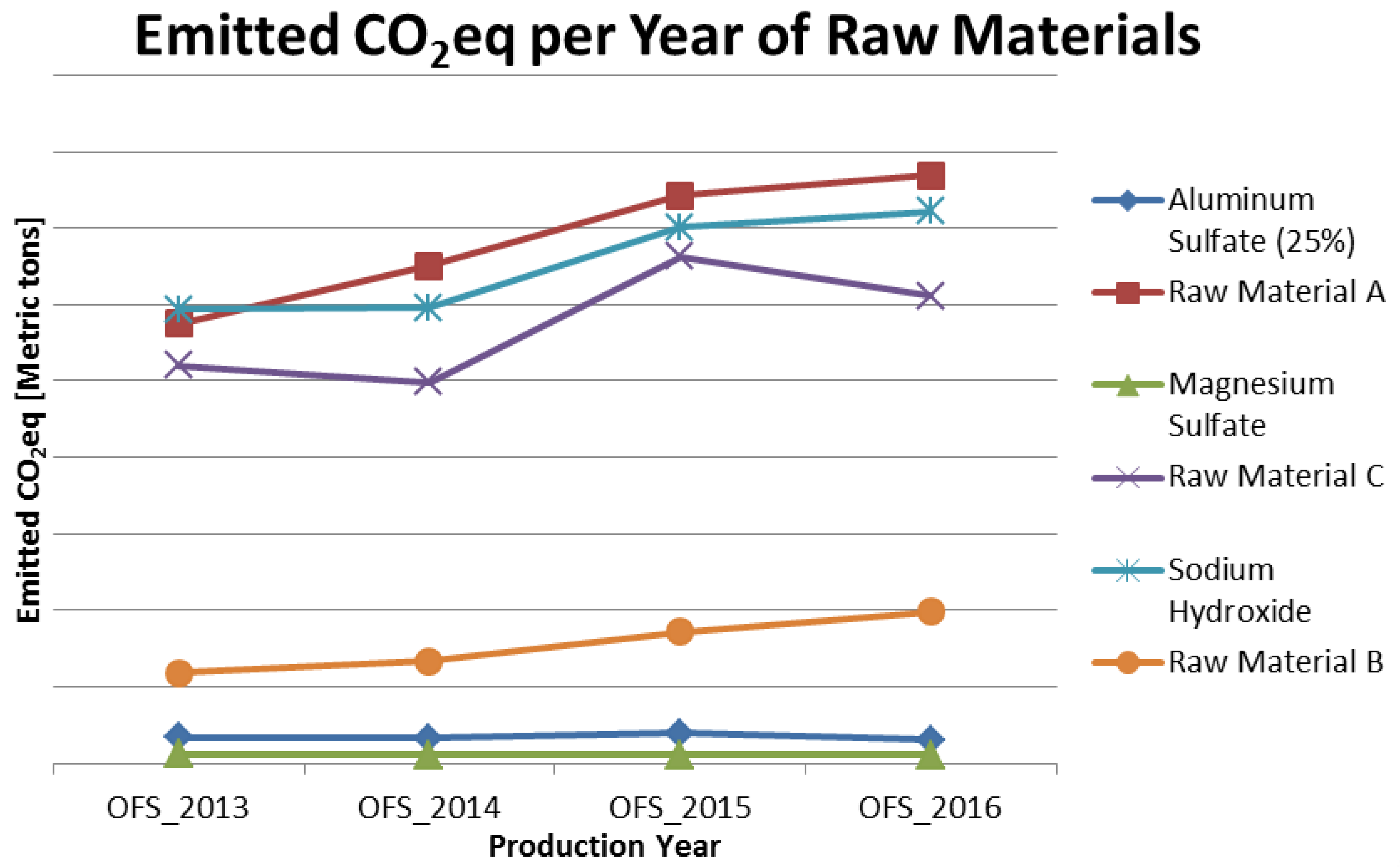
Figure 6 illustrates the six main raw materials used for the manufacturing of optical fiber and compares their emission rates per year considering a cradle approach. Because of an increase in production from 2013 to 2016, more raw materials had to be bought. When more of these raw materials are bought, the Scope 3 emissions increase. Note that the y-axis of Figure 6 is blank for security purposes.

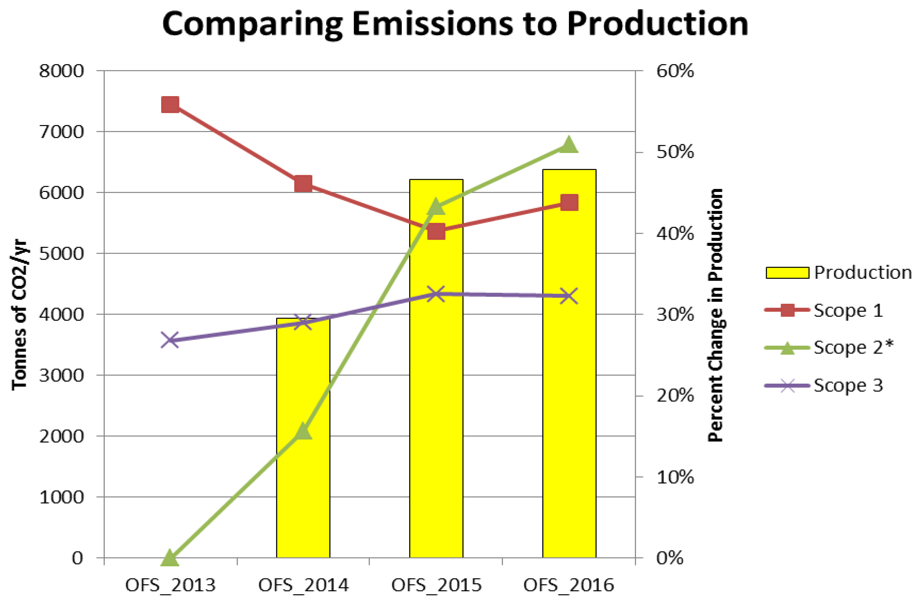
Also, correlations between carbon emissions and production of fiber were analyzed. Each of the major raw materials was also analyzed for emission increases or decreases per year of production. Figure 7 compares and illustrates the correlation between amount of fiber in million meters of fiber (FMM) produced and emissions for each specific scope. This figure exemplifies the how Scopes 1, 2 and 3 emissions change with the change in production. The figure shows an increase in production of fiber, a decrease in Scope 1 emissions and an increase in Scope 2 and 3 emissions. The increase in Scope 3 makes sense as it takes more raw materials to make more products. The interesting point of this graph is that as production increased, Scope 1, or direct emissions from the plant, decreased. This shows that OFS has been innovating to reduce their impact environmentally. It is also interesting to point out that Scope 2 increases by about 10% from 2013 to 2016. Scope 2 values on this graph are a representation of its magnitude, but not its scale as all emissions were subtracted from by the emissions from 2013.

Challenges

Many of the challenges in calculations arise from Scope 3 calculations of purchased goods. To find out the amount of carbon emissions generated by purchased goods, one only needs to know the quantity purchased and the emission factor of the product. An emission factor is a factor that can convert units of product purchased into units of CO₂ emitted by a certain amount of product. The best way to determine the emission factor of a product is to ask the manufacturer, as they should have a sustainability report that might have that information. Unfortunately, none of the companies that OFS purchases raw materials from has this specific information about their products. So instead, OFS had to use generic emission factors found in literature for each of its raw materials. Aluminum sulfate’s emission factor was the emission factor for the powder and not the liquid 25% by mass material that OFS uses. Raw Material A used at OFS has similar manufacturing properties as plastic, so the emission factor used is an average of different plastics’ emission factors. Raw Material C’s emission factor was difficult to find, so the emission factor used was that of a silicone product as they are both similar products. The emission factor for Raw Material B was very difficult to find, so instead, OFS used the emission factor of a generic chemical, which is 3 kg/kg. All of these numbers besides Raw Material A’s emission factor came from Appendix 7 of the WSTP South End Plant Process Selection Report [16]. Raw Material A’s emission factor was from Exhibit 8 of the plastics report by the United States Environmental Protection Agency [17].

4. Discussion

There were a few noteworthy portions of the results that are correlated with current attempts at the plant to be more environmentally conscious and more efficient with our energy. From 2013 to 2016, the amount of carbon emissions from the natural gas boilers decreased. This is due in part because of implementing improved maintenance practices, an energy assessment being done on all the boilers, and a full replacement of a boiler at the end of 2013 to a more energy efficient one. Another project to try to improve the carbon footprint is to replace all of the 36 electrical zirconium furnaces to more energy efficient graphite furnaces as their idle power suck is half that of a zirconium furnace. From 2013 to 2016, 12 of the 36 have been replaced. There is an increase in electricity usage for those four years, which is most likely a consequence of the 48% increase in production. In comparison, electricity usage was only up 10% from 2013 to 2016. It is however important to note that taking on large energy efficiency projects does cost a company a significant amount of money. For example, the transfer from zirconium furnace to graphite furnace costs $312,000 per furnace switch. As prior mentioned, from 2013 to 2016, 12 of the 36 have been replaced, which means $3.744 million was spent replacing those furnaces. Accounting for a 47.81% increase in production to the nominal increase in electricity output of 10.40%, electricity output for the plant was down 37.41%. Knowing that per year OFS spends about $7 million dollars on electricity, OFS saved $2.62 million in 2016 alone compared to 2013. Though it seems like a large expense, it turns out that if this trend continues, OFS can expect this switch to save the company $1.496 million by the end of 2017. And these savings will continue to improve the company’s bottom line for years to come. This is why it is very important to also look at the cost-benefit analysis of any energy-saving and environmental-helping causes, as they tend to be surprising.

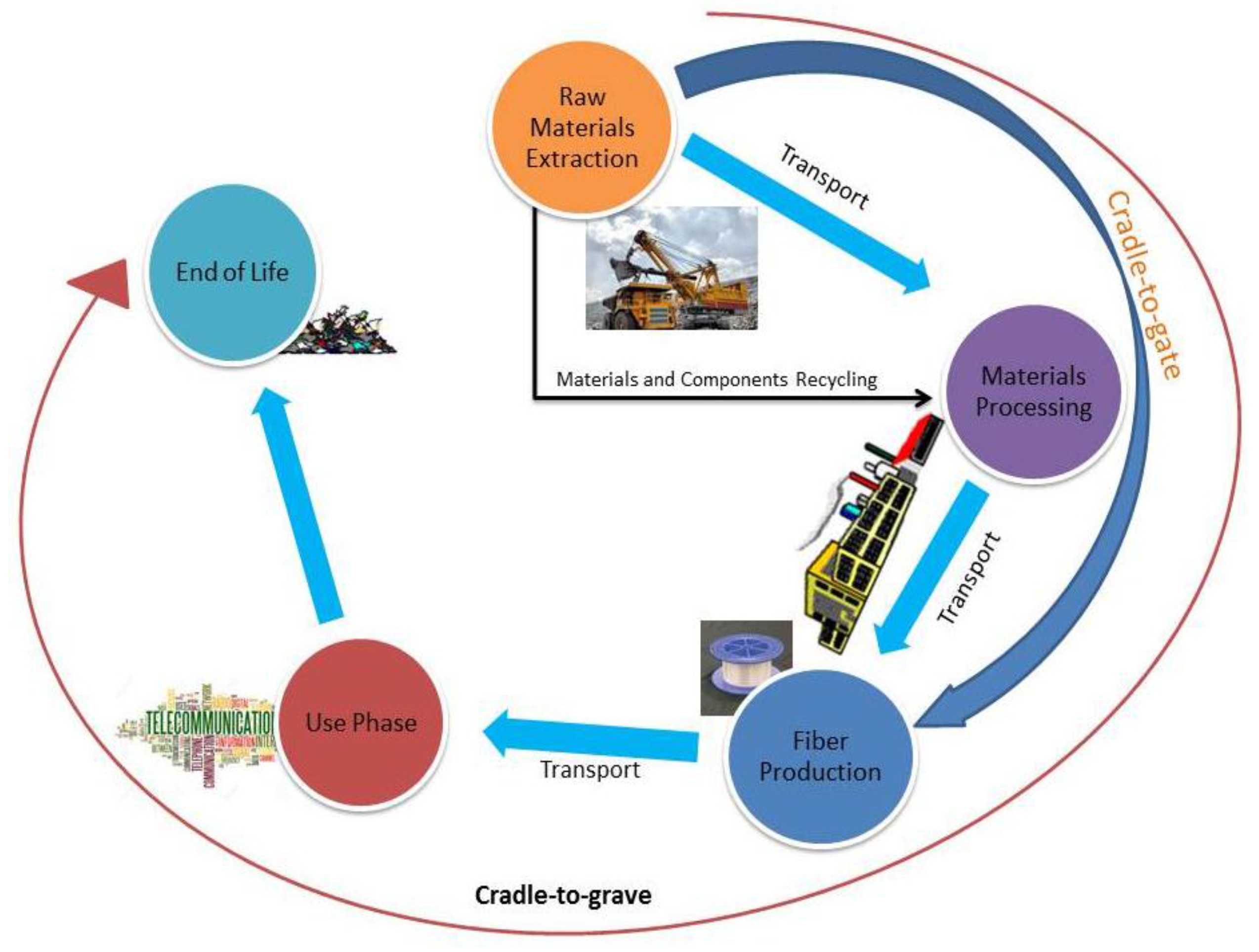
In general, the industrial sector produces goods for consumers by using energy to transform materials into useful products. Traditionally over the years, manufacturing systems have been designed based on a linear model starting with raw material extraction and ending with landfill disposal. A circular economy model challenges this approach by providing opportunities to re-manufacture and reuse end-of-life consumer products, leading to more efficient use of materials. By analyzing the pathways and transformations that occur as materials cycle from nature through manufacturing systems, industries have the opportunity to better understand the material requirements, reuse, and the associated use of energy and production of byproducts, waste products, and emissions to air, water, and soil. Carbon foot-printing by energy usage is the first step for this circular approach. No published literature is available for optical fiber production, as the carbon efficiency evaluation of Fiber to the x (FTTX) deployment currently excludes optical fiber production in calculations [18]. Based on the published FTTX L model, the amount of CO₂ emitted due to the use of fibers is far less than the amount of CO₂ that is emitted during the manufacturing; in fact, the former amount is several times lesser than the later, according to our calculations. That is why OFS uses every opportunity in all functional areas to develop products that not only function well but also have higher energy efficiency thereby emitting less CO₂ when used. In a wide range of fields, from manufacturing to FTTX, the OFS intention is to make products that help customers to reduce their environmental impact.

Perhaps, telecommunication industries are also being asked to make their networks “greener” as part of the overall push toward sustainability in business. Spending to bring information technology activity across the world into a greener space is expected to be significant. With reference to the data center market alone, Pike Research reports [19] that the amount of money spent to make data centers greener over the next four years will grow to $45 billion by 2016, at a compound annual growth rate of nearly 28 percent [20]. Optical fibers play very important role in tallying the carbon emissions from every part of a fiber to the home (FTTH) lifecycle, and in addition the optical fiber manufacturers are also able to spot places where reductions might be made. Since fiber networks use less energy to power the signal, they also generate less heat, and therefore require less cooling. Based on the EPA report [21], each kilowatt of network power in a data center requires a kilowatt of power for the cooling devices. Therefore, reducing energy use by powering a fiber-optic network will indeed need less energy to cool. This also means that data centers need less heating/ventilation/air-conditioning (HVAC) equipment in addition to the energy savings, year after year. Several key studies are reported expressing carbon footprint for FTTX deployment using life-cycle analysis (LCA), but the purifying and drawing of optical fiber in its production were excluded in those studies and no meaningful carbon footprint numbers exists in the literature yet.

The carbon footprint associated with making optical fibers is immensely complex and requires a comprehensive LCA, proceeding from raw material extraction and transportation to manufacturing (or service provision), to distribution, to consumer use, and to end-of-life disposal. Pure silica glass is the major component of optical fiber, and this pure silica has to be dug out of the ground. The silica has to be turned into SiCl₄. Other components have to be brought together: coatings, inks, several gases like hydrofluoric acid, and so on. All of this involves transporting things around the world. However, the different raw materials coming into a production process can be produced in different countries. The whole lot then has to be processed in a controlled environment, and every stage in the process requires lots of energy. So far, the available studies and methods for defining a fiber carbon footprint are far from comprehensive. More detailed, robust analytic techniques are in high demand as companies receive customer requests and regulatory pressure for this information. In addition, LCA efforts by nature can be resource-intensive, complex, and fraught with uncertainty due to the dynamics of supply chains, multitude of parts within a product, and lack of key data.

Fully leveraging on high technological prowess and comprehensive strength, OFS seeks to contribute even further to creating low carbon manufacturing which is sustainable at higher level.

Future Research

LCA study should also be performed on the environmental impact of all OFS products and services throughout their life spans. The LCA study provides OFS with a methodology to evaluate and quantify the impact of a product throughout all life-cycle phases and then makes decisions on how to reduce the impacts in each life cycle phase to optimize the environmental performance of the product.

Another study to consider would be a study that compares the emissions from the production to the emissions from the actual usage of the product and tries to balance making the production more environmentally friendly and to make improvements to the final product for better performance. This would increase the scope of this paper to cradle-to-grave.

5. Conclusions

Overall, OFS has some work to do in order to compete within the growing culture of environmental friendliness. The overall emission factor for optical fiber production decreased from 2013 to 2016, with the 2016 number being 4.81 CO₂eq emitted per million meters of optical fiber produced, or 72.92 kg CO₂eq emitted per kg of optical fiber produced. Scope 1 emissions at OFS have been going down in the past few years, but Scope 2 emissions have increased significantly to the point where it has increased the specific GHG of optical fiber produced. OFS has many opportunities to lower emissions within the combustion portion of their process and their energy usage portion. They also have the option to look for more sustainable raw materials to help decrease their environmental footprint and increase their overall profits. The world is experiencing a cultural shift and encouraging more environmentally friendly activities, which means that information on how to quantify and help the environment should be readily available to all companies.

References

1. The Economics Intelligent Unit. The Cost of Inaction: Recognizing the Value of Risk from Climate Change, Sponsored by Aviva; EIU: London, UK, 2015. [Google Scholar]
2. List of Parties that Signed the Paris Agreement on 22 April. Available online: http://www.un.org/sustainabledevelopment/blog/2016/04/parisagreementsingatures/ (accessed on 22 April 2016).
3. Furukawa Electric Group: Products. Available online: https://www.furukawa.co.jp/en/product/catalogue/pdf/e03.pdf (accessed on 1 May 2017).
4. International Organization for Standardization. ISO/TS 14067:2013, Greenhouse Gases—Carbon Footprint of Products—Requirements and Guidelines for Quantification and Communication; ISO: Geneva, Switzerland, 2013. [Google Scholar]
5. Chan, C.A.; Gygax, A.F.; Wong, E.; Leckie, C.A.; Nirmalathas, A.; Kilper, D.C. Methodologies for Assessing the Use-Phase Power Consumption and Greenhouse Gas Emissions of Telecommunications Network Services. Environ. Sci. Technol. 2013, 47, 485–492. [Google Scholar] [CrossRef] [PubMed]
6. Fuhr, J.P., Jr.; Pociask, S.B. Broadband Services: Economic and Environmental Benefits; The American Consumer Institute Center for Citizen Research: Washington, DC, USA, 2007. [Google Scholar]
7. DCEP: Data Center Electricity Productivity. 42u. Available online: http://www.42u.com/measurement/dcep.htm (accessed on 1 May 2017).
8. Baliga, J.; Ayre, R.; Hinton, K.; Sorin, W.V.; Tucker, R.S. Energy Consumption in Optical IP Networks. J. Lightwave Technol. 2009, 27, 2391–2403. [Google Scholar] [CrossRef]
9. The Growth in Global Telecom GHG Emissions. Vertatique-Green ICT: Sustainable Computing, Media, e-Devices. 2014. Available online: http://www.vertatique.com/telecom-emissions-300-mtco2-and-growing (accessed on 1 May 2017).
10. Lange, C.; Gladisch, A. Improving the Energy Efficiency of Telecommunication Networks; Deustsche Telekom Laboratories: Berlin, Germany, 2011. [Google Scholar]
11. Code of Federal Regulations. 40CFR98, Protection of Environment: Environmental Protection Agency: Air Programs: Mandatory Greenhouse Gas Reporting; U.S. Government Publishing Office: Seattle, WA, USA, 2011.
12. Greenhouse Gas Protocol: Calculation Tools. Available online: http://www.ghgprotocol.org/calculation-tools (accessed on 1 May 2017).
13. Ungar, S. Fibre Optics: Theory and Applications; John Wiley & Sons, Inc.: New York, NY, USA, 1990. [Google Scholar]
14. Freudenrich, C.C. How Fibre Optics Work. Instrument Design. Available online: http://instrumentdesign.blogspot.com/2007/05/how-fiber-optics-work.htmlhtml (accessed on 1 May 2017).
15. How Much Electricity does an American Home Use? U.S. Energy Information Administration. Available online: https://www.eia.gov/tools/faqs/faq.cfm?id=97&t=3 (accessed on 21 October 2015).
16. Emission Factors in kg CO2-Equivalent per Unit City of Winnipeg. Available online: http://www.winnipeg.ca/finance/findata/matmgt/documents/2012/682-2012/682-2012_Appendix_H-WSTP_South_End_Plant_Process_Selection_Report/Appendix%207.pdf (accessed on 1 May 2017).
17. Plastics. Available online: https://www3.epa.gov/epawaste/conserve/tools/warm/pdfs/Plastics.pdf (accessed on 1 May 2017).
18. Griffa, G.; Andrae, A.S.G. Carbon Efficiency Evaluation of FTTx Deployment Huawei Communicate; Huawei Publications: Liebefeld, Switzerland, 2010. [Google Scholar]
19. Pike Report. Green Data Center Market to Surpass $45 Billion by 2016; Navigant Research: Boulder, CO, USA, 2012. [Google Scholar]
20. Kaplan, J.M.; Forrest, W.; Kindler, N. Revolutionizing Data Center Efficiency; McKinsey and Company: New York, NY, USA, 2008. [Google Scholar]
21. USEPA (United States Environmental Protection Agency). Report to Congress on Server and Data Center Energy Efficiency: Public Law 109-431; USEPA: Berkeley, CA, USA, 2007.
Figure 1. A visual of the Life-Cycle Assessment of optical fiber.
Sustainability 09 00865 g001
Figure 2. A generalized illustration of the activities, inputs, and outputs associated with optical fiber manufacturing to be considered in the scope of carbon footprinting.
Sustainability 09 00865 g002
Figure 3. Schematic Drawing of the Vapor-Phase Axial Deposition (VAD) Glass Core Manufacturing Process [13].
Sustainability 09 00865 g003
Figure 4. Diagram of a fiber drawing tower used to draw optical glass fibers from a preform [14]. UV in the figure above stands for Ultraviolet light.
Sustainability 09 00865 g004
Figure 5. A drawing of the layout of a Rewinder.
Sustainability 09 00865 g005
Figure 6. A graph showing the amount of emitted carbon emissions per year for the major raw materials of the optical fiber industry.
Sustainability 09 00865 g006
Figure 7. A comparison of the production amount of wire per year to that of Scopes 1, 2 and 3 emissions per year. * Note that Scope 2 has been altered so OFS_2013 is equal to 0, OFS_2014 is equivalent to Scope 2 in 2014 minus Scope 2 in 2013, etc. This was done so the magnitude of Scope 2 could be preserved on this graph.
Sustainability 09 00865 g007