The Impacts of Technical Progress on Sulfur Dioxide Kuznets Curve in China: A Spatial Panel Data Approach

Abstract

This paper aims to reveal the nexus for sulfur dioxide (SO₂) emission and income, as well as the effects of technical progress on SO₂ emission in China based on environment Kuznets curve (EKC) hypothesis. The spatial panel technique is used in case the coefficient estimates are biased due to the negligence of spatial dependence. With the provincial panel data of China from 2004 to 2014, this is the first research that finds an inverse N-trajectory of the relationship between SO₂ emission and economic growth and confirms the beneficial impacts of technical advancement on SO₂ emission abatement. The empirical results also suggest that the industrial structure change is an important driving force of the SO₂ EKC. In addition, the direct and spillover effects of determinants on sulfur emission are clarified and estimated by a correct approach. Finally, we check the stability of our conclusions on the EKC shape for SO₂ and technical progress effects when controlling for different variables and specifications, through which we find the turning points are sensitive to variables selections.

1. Introduction

Interest in economic growth and environmental deterioration nexus has constantly increased among economists, ecologists and policymakers as it is meaningful and informative for the pollution abatement policies and economic development. The environment Kuznets curve (EKC) hypothesis raised a theoretical framework for the research of the relationship between development and environment degeneration. The traditional EKC hypothesis suggests an inverted U-shaped curve between environmental deterioration and economic development that describes the increase of the ambient pollution in the early stage and the decrease of the environmental deterioration after the turning point (threshold) [1]. Therefore, the validity of the EKC can offer a way out for the dilemma of economic growth and environmental preservation, especially among the currently developing countries. The traditional EKC theory also holds that the technological impact is one of the reasons that contributes to the declining of environmental deterioration along with the development [2].

China, as a developing country, has had continuous economic boost in past decades, which draws a significant amount of focus on its sustainability of development and concerns on its environment. Chinese annual economic growth rate peaked at 14.6% in 2007. With such a rapid growth, the energy consumption was inevitably massive. As a result of China’s heavy dependence on coal energy and secondary industry, SO₂ is one of the major exhaust gas pollutants and its emission volume reached the top at 25.94 million tons in 2006 [3]. In 2006, Chinese government set a series goals aiming for cutting the pollutants emission by 10% during the 11th Five-Year plans period. The total SO₂ emission deduced by 12.45% based on the 2005 emission level. However, the amount of SO₂ emission is still a heavy burden on the environment system: in 2010, 21.85 million tons of SO₂ were exhausted into the atmosphere [4]. On the other hand, China has increased investment in new energy industries and environmental technologies such as wind power, hydropower, solar power and end-of-pipe abatement technology that can largely reduce exhaust gas emission [3,5]. Thus, except for the economic factors, the technical progress impacts on SO₂ emission in China are another issue worthy of discussion.

In the past literature, multiple shaped environmental Kuznets curves such as U, inverse U-shaped, and N were found [6]. Zheng et al. [7] and Kang et al. [6] testified an inverse N-shaped EKC for carbon dioxide emission in China. Because an U/inverse U-shaped EKC is naturally nested in an N/inverted N-shaped EKC, in this study, we examine if there exists an N or inverse N-shaped EKC for SO₂ emission in China.

To take the spatial dependent effects of variables into account, these two prior studies focused on CO₂ ECK in China and applied the spatial panel data models: Zheng et al. [7] applied the dynamic spatial panel model to explore the determinants and spatial relation of provincial carbon dioxide emission in China. They firstly found the inverted N-shaped relationship between carbon dioxide intensity and GDP in China, yet they failed to present the amount of direct and spillover effects of those determinants. After that, Kang et al. [6] further testified the inverse N-shaped relationship between carbon dioxide emission and GDP through the application of spatial panel data technique. Besides, they also reported two turning points of the inverted N-trajectory. However, they directly interpreted the coefficients estimates of independent variables in spatial Durbin model as the direct and spillover effects, which is invalid. LeSage and Pace [8] argued that the estimated coefficients of spatially lagged explanatory variables and its significant test should not be explained as the amount of spillovers and significance of spillover effects in spatial models. Instead, a partial derivative estimate of the impact of changes in the variables in spatial model specification offers a more valid way of estimation and interpretation of spillover effects and testing significance. Furthermore, Elhorst [9] pointed out that parameters estimated in the spatial Durbin model do not represent the direct marginal effects of a change in the explanatory variables on the dependent variable, since the feedback effects (Feedback effect = Direct effect − Coefficient) will lead to a impacts going through neighboring regions and then back to the local regions themselves. To the best of our knowledge, no one has studied the spillover effects in the EKC for SO₂ or examined the existence of the cubic term in the SO₂ EKC in the context of China. In addition, the technical progress impacts on the reduction of SO₂ emission remains uncertified. Therefore, this study contributes to the literature by overcoming these gaps. There are four unique contributions of this paper. First, we verified the existence of the inverse N-shaped EKC for SO₂ and its stability in the context of China. Second, we clarified the beneficial effects of technical progress on SO₂ emission reduction and its stability. Third, the industrial structure is confirmed to be a driving force of SO₂ EKC. Fourth, a valid estimation approach is applied for the direct and spillover effects of the determinants of SO₂ emission through spatial panel data model.

The remainder of the paper is organized as follows: Section 2 gives a brief review of past literature. Section 3 describes the variable selection for the empirical analysis and methodologies of spatial econometrics. Section 4 describes the details and source of the data. Section 5 presents the estimation results and analysis. Section 6 conducts the robustness check to test the stability of estimation results in different situations. Section 7 concludes our findings, presents the limitations and offers implications for further studies.

2. Literature Review

Grossman and Krueger’s study [1] was the first economics research that introduced the environment Kuznets curve (EKC) hypothesis. They suggested the existence of an inverse U-shaped relationship between pollutants and economy growth based on the study of 42 countries. Later, Holtz-Eakin and Selden [10] and Stern [11] verified the EKC hypothesis for carbon dioxide emission. After examining gasoline data in 48 countries, Hilton and Levinson [12] found that the functional form, time period and technique effects influence the turning point of EKC for vehicle emissions. Kaufmann et al. [13] and List and Gallet [14] testified this hypothesis for SO₂ emission and concluded that the inverted U-shape EKC generally described the relationship between SO₂ emissions and personal income at the state level. Harbaugh et al. [15] explored the EKC hypothesis for SO₂ and TSP through the panel data model with fixed effects specification and found the result was sensitive to econometric model specification, functional form, countries studied and the years covered. Miah et al. [16] investigated and testified the inverted U-shaped EKC hypothesis for the primary gas pollutants: carbon, sulfur, and nitrogen dioxide.

Fodha and Zaghoud [17] focused on the heterogeneity of different types of gas pollutants of EKC. Their findings also support an inverted U-shaped EKC for SO₂ emission. Some other indicators of the economy were also considered: Cole [18], and Cole and Neumayer [19] studied the relationship between environmental degeneration and urbanization in 86 countries. Zhang and Lin [5] examined the effects of urbanization on carbon dioxide (CO₂) emission in three parts, eastern, western, and central of China. In the past decades, some advanced methodologies were also used for exploring EKC. Taskin and Zaim [20] used the nonparametric kernel regression technique to explore CO₂ emissions in 52 countries from 1975 to 1990. They concluded an inverted N-shaped nexus between CO₂ emission and economic growth with two turning point: $5000 and $12,000 per capita. Stern [11] investigated 82 countries from 1971 to 1990 and testified the EKC for SO₂ emission by the panel data approach. Shen [21] applied the panel data model and confirmed a U-shaped EKC path for SO₂ emission in China based on 10 years of provincial data. Maddison [22] used spatial econometric models to examine the EKCs for sulfur, carbon and nitrogen dioxide and volatile organic compounds with the data of 135 countries. Not surprisingly, the spatial interaction between the local and adjacent countries was detected by him; that is, the assumption of the independence of cross-sectional data is not valid.

In addition, Kaika and Zervas [23,24] pointed out that except for economic factors, technical advancement, and international trade are also the potential determinants in the framework of EKC for CO₂. Wang et al. [25] argued that technology spillovers, trade openness and policies are the causes for the spatial dependence. Yin et al. [2] testified the beneficial effects of government’s regulation and technical progress on CO₂ emission plus an inverse U-shaped EKC for CO₂ in China. Wang et al. [26] verified an inverse U-shaped ECK for SO₂ emission on the Chinese context. Moreover, Zheng et al. [7] and Kang et al. [6] found an inverted N-shaped nexus between CO₂ emission and economic growth in China through spatial panel data model.

The Environmental Kuznets Curve hypothesis has raised doubts and critiques among scholars as well as policymakers and those critiques focus on both the concept of EKC and methodology in past studies.

The inversely U-shaped EKC does not fit for all kinds of pollutants. Little empirical evidence is found supporting an inverse U-shape EKC for several important air pollutants [15]. The EKC hypothesis is most plausible for various environmental indicators of air pollutants (e.g., suspended particulate matter (SPM) and SO₂). However, the EKC relationship is only verified for the air pollutants such as SPM, SO₂, CO, etc., that are associated to short-term environmental impacts in local areas, not for the accumulated pollution that has long-term and dispersed effects and positive relation with income level. For instance, the EKC does not explain income–CO₂ emission relationship in any reasonable way [10,27,28]. Through the examination on a panel of 149 countries from 1960 to 1990, Shafik and Bandyopadhyay [29] found that only two of ten indices of environmental quality followed an EKC path. Ambient levels of SPM and SO₂ concentration showed inverted U trajectory, whereas dissolved oxygen, total deforestation, deforestation rates, clean water, fecal coliform, municipal waste, urban sanitation and CO₂ emissions per capita did not [30]. In addition, the land-use change and bio-diversity loss are essentially different from air and water pollution due to the irreversibility. Thus KEC should not hold for land-use and bio-diversity loss [28].

A number of early EKC studies analyzed cross-sectional data and concluded a unique development paths existing among different countries/regions, which has been criticized for the invalidity of cross-sectional technique [14,31,32]. For instance, a group of countries may experience environmental degeneration with increasing economic development, while other countries (in the same study) may go through environmental improvement with growth in economy. One may derive an inverted-U shape from a cross-sectional regression that mix these two different groups of sample together. However, such an inversely U-shaped curve does not depict the paths of any countries in these two groups [33].

Bradford et al. [34] suggested that per capita income and per capita emissions (and logarithmic transformations of their value) are commonly regarded as non-stationary unit root processes, thus nonstationary econometric techniques (panel unit root and panel cointegration tests) are usually utilized in panel data EKC studies (e.g., [19,35,36,37]). Nevertheless, so far, the validity of panel unit root tests generally rely on the pre-assumption of i.i.d (independent and identically distributed) sampling, which is not practical in most empirical research. Another problem lies in the logarithmic transformations of the dependent and independent variable in unit root process due to the fact that nonlinear transformations on unit root process changes the process’s stochastic characters in essence [38]. However, some of the prior research ignored these problematic issues when taking the potential unit root process (in panel data) into account [33]. Considering the reason that panel data in the following empirical analysis might be nonstationary, we mainly focus on the results from regression that controls for time or both spatial and time effects, since the inclusion of time trend in panel regression model can more or less offset the nonstationary problems and avoid spurious regression. Dijkgraaf and Vollebergh [39] studied the heterogeneity of carbon dioxide emission among the OECD countries through the panel data model. They criticized the homogeneity assumption of the EKC for different countries and argued that no general cross-country EKC path exists.

Other critiques also focused on the robustness of EKC relation in empirical analysis. The value and significance of parameter estimates are highly sensitive to variable selection and models specification [15]. Some studies adopted reduced form that directly link development and environmental impacts to explore EKC relation (e.g., [1,40]), rather than structural form models to control for other potential factors (e.g., technology, abatement, energy consumption, regulations, industrial structure, etc.) that associate environmental quality with the economic growth. Apparent, reduced model specifications are more concise and can reduce the work of data collection for independent variables and consumption of degree of freedom. Clearly, endowments of countries/local regions influence environmental quality thus structural forms may have more explanatory power. Whereas reduced form models are of limited function in revealing causal mechanisms [28,30,37]. Besides, variables selection and model specification significantly affect the shape of EKC estimation [30]. This is the reason we conduct the robustness check of the EKC estimates in Section 6. In addition, Ansuategi et al. [41] and Copeland [42] pointed out that other relevant factors were inadequately omitted in some of the EKC studies. Trans-boundary externalities (e.g., migration and technology spillovers) are one kind of factor. In addition, abundant empirical evidence suggests that, in Asia and Latin America, adjacent regions have significant influence on environmental behaviors of local factories [43,44,45,46].

Above all, to explore the possible EKC path for SO₂ emission and the spatial spillovers (trans-boundary externalities) across provinces, the current study utilized the most recent SO₂ emission dataset at the provincial level in China (2004–2014) and the recent developed spatial panel data model for the empirical analysis. Other than that, we illustrated OLS estimates and conducted the Moran’s I and LM tests to make our model specification more valid for controlling for spatial dependence. Finally, we checked the stability of the results and shed new light on further related studies.

3. Theoretical Framework and Methodological Approach

3.1. EKC Model

The following reduced polynomial function is constantly utilized to test various possible income–environmental quality relationships:

$$Y=\alpha +{\beta }_{1}X+{\beta }_2{X}^2+{\beta }_3{X}^3+{\beta }_{4}Z+\epsilon$$

(1)

where β are the coefficients of independent variables, Y is environmental quality indictor, X is income (usually GDP per capita) and Z represents other influential factors on environment. Equation (1) enables us to test the forms of income–environmental quality relationships:

(a)

β₁ = β₂ = β₃ = 0: No relation for X and Y.

(b)

β₁ > 0 and β₂ = β₃ = 0: A linear relationship (monotonic increasing) between X and Y.

(c)

β₁ < 0 and β₂ = β₃ = 0: A linear relationship (monotonic decreasing) between X and Y.

(d)

β₁ > 0, β₂ < 0 and β₃ = 0: An inversely-U-shaped relation, i.e., the classical EKC.

(e)

β₁ < 0, β₂ > 0 and β₃ = 0: A U-shaped relation.

(f)

β₁ > 0, β₂ < 0 and β₃ > 0: An N-shaped curve.

(g)

β₁ < 0, β₂ > 0 and β₃ < 0: An inversely N-shaped curve.

Equation (1) (or the logarithmic value of the variables in Equation (1)) is applied in the bulk of literature through econometric techniques for the exploration of an EKC for various indices of environmental degeneration.

3.2. Model Specification

We referred to Stochastic Impacts by Regression on Population, Affluence, and Technology (STIRPAT) model and the pollution haven hypothesis to choose proper independent variables. We also considered data quality and availability.

Some researchers disagree with the traditional inverse U-shaped EKC, especially when longer-term time scales are evaluated [47]. For example, Millimet et al. [48] concluded that inverse U-shaped curve was actually an N-shaped curve, which means pollution increases while a country develops in an early stage. After the threshold GDP is reached, it decreases, and then starts to increase while income keeps increasing. To test such a possible shape of EKC for SO₂ in China, we naturally incorporate a cubic term of the affluence into the model. The addition of a cubic term of affluence factor implies that an N-shaped or inverse N-shaped curve might exist between SO₂ emission and economic development.

To bear this in mind, focus of the study lies on the technical progress impacts on SO₂ emission, therefore explicit elaboration of related underpinning and mechanism is necessary. Many authors pointed out that technical progress is a fundamental driving force of the environment Kuznets curve (e.g., [49,50,51]). The source of EKC can be categorized into two groups: technological progress and structural change [28]. Highly advanced technology in the long term is likely to be the primary cause of environmental quality improvement [52]. Dinda et al. [50] suggested that SO₂ emissions have decreased over time probably due to technological progress. De Bruyn [53] also empirically confirmed that technological progress is relatively more important for explaining reduce of SO₂ emission in both Netherlands and West Germany. Theoretically, technological advancement improves the efficiency in utilization of energy and materials during production, which can lessen burdens on environment as well as reduce consumption of natural resource when producing the same amount of goods. Renewable energies accompanied by the advancement may also enable recycling of production materials and more efficient reuse, by which a community can reserves more natural resources [28].

Technological update not only largely escalates efficiency on manufacturing old goods but also develops new products. A prevailing inclination among industrial fields indicates that industries also consider environmental outcomes of their production during production processes, which influence the aspects of old technologies, the production organization and the products design. Technological changes in production process may lead to changes in the input combinations of materials as well as fuels in the process [54]. The substitution of materials and fuels could play an important role in advance economics [55] that help to lower pollution level. The wide ranging economic reforms not only promote the economy and society but also environment quality [56,57].

In addition, as income increases, the public starts to prefer efficient technology that can lead to environmental improvement. People’s income elasticity can reflect such preference and the income elasticity of public R&D and expenditure on environmental protection is always positive [58]. This has been confirmed by the empirical analysis [59] of 19 OECD countries’ public investment on R&D for the sake of environmental protection during 1980–1994.

Regarding the technical effects, there exists abounding exemplars of efficient resource use, resource replacement, and pollutants abatement in developed countries. One of most impressive is SO₂ emission abatements in France, Germany and Japan through the substitution of nuclear power (France), the installation of sulfur removal device for flue-gas (Germany), and a combination of the first and second (Japan) [28]. Although no consensus of the proxy for technology advancement and innovations exists, patents play an important role in the progress of technology development. Moreover, patents application/authorization is the most broad indicator of innovative technology used by scholars in their research [60,61].

Another significant factor that has always been considered is population [49,52,62]. Apparently, the existing literature indicates that most population in the world lies on the upward phase of EKCs, and the increase of population pressure can also give rise to environmental degeneration [63]. Economic activities not only generate wealth in society but also bring environmental pressure. The producing and manufacturing process in industrialized countries discharge considerable waste and pollutants that deteriorate environment in which people live. Such environmental impacts could be more serious if accompanied by larger population size since the larger size lead to more energy consumption, consequently, to more severer ambient pollution [64]. A community with a larger population size is likely to dispose more solid wastes through incineration and consume more local resources such as food, clothing, transportation, fuel cooking and heating, etc., which are energy and emission intensive. In a technological/agrarian community, each human individual exerts negative effects on the environment around him/her. S/He contributes to the destabilization of ecological system. S/He also consumes renewable as well as nonrenewable resources. The whole deteriorating effects on environmental system from population in the community can be described in a concise form, by the equation I = PF(p), where P is the total population and F is a function of per capita impacts on environment [65]. Besides, the adverse effects from population was also detected in the past empirical studies of China’s air pollutants (e.g., [3,66]). Thus, the population size enters the following models as an explanatory variable. It is noteworthy that, some scholars [4,6,67] used population density as the proxy of population effects, by which one could take the size effect of provincial land area into account. We also test this indicator in one of the model specification (Equation (6)) and present the related discussion in Section 6.5.

Following the Pollution Haven Hypothesis (PHH), we incorporate trade openness in the regression model. The PHH suggests that multinational firms (from developed countries), especially those participate in activities with heavily polluting outcomes, tend to relocate their industries to less developed countries because of the incentives of lower environmental protection standards in these countries. Less developed countries are termed “pollution haven” in the PHH, if their environmental standards are below the level of efficiency for attracting foreign capital and investment. Indeed, lower trade barriers may deteriorate environment when heavy pollution shift to countries that have weaker regulations [18,68,69,70,71].

The relationship between pollutant emissions and urbanization is another widely concerned issue. Previous studies illustrated conflicting results on this theme, indicating that the relationship between urbanization and environment is complicated. Some scholars argue that higher urbanization level is usually accompanied by more energy demand that generates more pollutants [19,72,73]. Modernization theorists also suggest that urbanization affects environment outcomes and can explain the EKC [64,74]. Rapid urbanization leads to considerable demand in building materials for upgrading and constructing new public infrastructure such as drainage system, road networks, water supply and sanitation, etc. These construction projects inevitably increase energy consumption and emission level at local areas. Besides, a growing number of immigrants from suburban areas to urban areas need larger scale of transportation system and consume more electricity (a major resource of industrial SO₂ emission). On the contrary, other researchers claim that a level up in urbanization or urban density lead to improvement in utilization efficient of public infrastructure such as public transport, which can decrease energy consumption, consequently reducing pollutants emissions [75,76]. It can also promote environmental improvement through economies of scale in services of sanitation and environmental protection [77]. These contradictory conclusions here might be explained by different characters in energy structure, income level, urban public service level, etc. [36]. Given the fact that China has been sprawling its cities and boosting the infrastructure construction in urban areas, we take the percentage of population living in urban areas as a proxy to stress the modernization theory and capture the possible urbanization effects on environmental quality.

The relationship between energy use and specific environmental index is a widely studied theme in the field of environment/energy economics. Although some literature uses energy intensity as the proxy of energy factors (e.g., [3,66]), we argue that some kinds of energy consumptions, such as natural gas and petroleum, included in energy intensity do not significantly attribute to SO₂ emission. Considering characteristics of current China’s composition of energy use, we control for coal and power consumptions in the model. China has been the largest consumer of coal in the world. In 2012, China consumed nearly half the world’s coal and the coal consumption accounted for 68.5% of its own total energy structure [78], while it heavily relies on thermal power generation, for example, its thermal power generation accounted for 78.0% of total power generation in the same year [79]. Coal combustion and thermal power generation both emit the bulk of SO₂.

Pollution intensities vary in different industries as the structure of production changes with economic growth. At the earlier stage of economic development, capital and source in agricultural sector transfer to heavy industry which promote pollutant emissions. When it comes to the later phases of development, a shift from heavy industrial/resource consuming sectors towards services/light manufacturing sectors takes place, which leads to lower emissions level [80]. Dinda [28] also hold a similar view: environmental deterioration is likely to become severe if economic structure changes from agricultural to industrial fields, however it would improve with later structural shift from energy/emission intensive fields to services and knowledge intensive fields in the due course. To capture such industrial composition effects, we introduce share of the secondary industry in GDP (SEC-GDP ratio) into empirical model. SEC-GDP ratio could measure the overall transformation of industrial structure in which a country undergo as its economy develops. One can expect rapid increases of the share of the manufacturing fields in industrializing communities, whereas the share tends to be stable or declining in industrialized communities. It is worth noting that a rise in the ratio implies more than merely a greater mass of energy consumed during industrial production. Particularly, it partially represents some associations of industrialization/urbanization and increasing transportation utility that can also spur the energy consumption in the community [81].

Accordingly, we estimated the empirical model as follow

$$\ln S{O}_2={\beta }_0+{\beta }_1\ln GPD+{\beta }_2{(\ln GDP)}^2+{\beta }_3{(\ln GDP)}^3+{\beta }_4\ln PA+{\beta }_5\ln POP+\epsilon$$

(2)

$$\ln S{O}_2={\beta }_0+{\beta }_1\ln GPD+{\beta }_2{(\ln GDP)}^2+{\beta }_3{(\ln GDP)}^3+{\beta }_4\ln PA+{\beta }_5\ln POP+{\beta }_{6}TO+{\beta }_{7}URBEN+\epsilon$$

(3)

$$\ln S{O}_2={\beta }_0+{\beta }_1\ln GPD+{\beta }_2{(\ln GDP)}^2+{\beta }_3{(\ln GDP)}^3+{\beta }_4\ln PA+{\beta }_5\ln POP+{\beta }_6\ln Coal+{\beta }_7\ln Electrc+\epsilon$$

(4)

$$\ln S{O}_2={\beta }_0+{\beta }_1\ln GPD+{\beta }_2{(\ln GDP)}^2+{\beta }_3{(\ln GDP)}^3+{\beta }_4\ln PA+{\beta }_5\ln POP+{\beta }_6\ln Sec+\epsilon$$

(5)

$$\ln S{O}_2={\beta }_0+{\beta }_1\ln GPD+{\beta }_2{(\ln GDP)}^2+{\beta }_3{(\ln GDP)}^3+{\beta }_4\ln PA+{\beta }_5\ln Popd+\epsilon$$

(6)

where SO₂ is the amount of SO₂ emission; GDP denotes the real GDP per capita, the proxy of affluence; PA is the number of patents applications examined, the proxy of technical progress level; POP represents the total population; TO refers to trade openness (expressed through the percentage of gross export and import to real GDP); URBEN stands for urbanization (measured by the ratio of the urban population to the total population); Coal stands for coal consumption, Electrc for electricity consumption; Sec for share of the secondary industry in GDP; and Popd for population density. $u$ is the error term. In these models, all variables except trade openness and urbanization were taken natural logarithm, so the coefficients ${\beta }_1$, ${\beta }_2$ and ${\beta }_3$ reflects the polynomial relationship (trajectory) between SO₂ emission and economic development while ${\beta }_4$, ${\beta }_5$, ${\beta }_6$ and ${\beta }_7$ can be directly interpreted as the elasticity (taken ${\beta }_4$ as an example, a 1% change on technical progress will lead to a ${\beta }_4\%$ change on SO₂ emission). In our model specifications, trade openness, urbanization, energies consumption, share of secondary industry and population density are control variables. Equation (2) is the basic model specification in our study, since we focus on the technical effects and Wang et al. [3] already found the evidences supporting population effects on SO₂ emission in China. Equation (2) will be estimated firstly. Thereafter, Equations (3)–(6) will be estimated to examine the stability of the basic results from Equation (2) and impacts of other variables.

3.3. Spatial Panel Data Model

Three types of spatial panel models were considered as the potential model specification in this study: the spatial Durbin, spatial lag, and spatial error models. The spatial Durbin model (SDM) can be written in matrix form as

$$Y=\delta (I_T\otimes W_N)Y+X\beta +\gamma (I_T\otimes W_N)X+({\tau }_T\otimes I_N)\mu +(I_T\otimes {\tau }_N)\eta +u,\hspace{1em}\hspace{1em}u\sim N(0,{\sigma }^2{I}_{NT})$$

(7)

The spatial lag model (SAR) can be written as

$$Y=\delta (I_T\otimes W_N)Y+X\beta +({\tau }_T\otimes I_N)\mu +(I_T\otimes {\tau }_N)\eta +u,\hspace{1em}\hspace{1em}u\sim N(0,{\sigma }^2{I}_{NT})$$

(8)

The spatial error model (SEM) can be written as

$$\begin{array}{l}Y=X\beta +({\tau }_T\otimes I_N)\mu +({\tau }_N\otimes I_T)\eta +u\\ u=\rho (I_T\otimes W_N)u+\upsilon \\ \upsilon \sim N(0,{\sigma }^2{I}_{NT})\end{array}$$

(9)

where $Y$ contains an NT × 1 vector of provincial level SO₂ emission. $X$ is an NK × K matrix of the independent variables which was illustrated on the right-hand side of Equations (2)–(6). The term $\mu$ indicates the individual effects among 31 Chinese provinces and $\eta$ refers to the time effects. ${\tau }_T$ indicates a column vector of ones of length T and ${\tau }_N$ indicates a column vectors of ones of length N. $\delta$ is the spatial autocorrelation coefficient and $\rho$ is the spatial autocorrelation that assumed to exist in the error term. Parameter $\beta$ shows the influence that the independent variables exert on the dependent variable. $\gamma$ is the coefficient that reflects the spillover effects of explanatory. $I_T$ is a T × T dimension identity matrix and $I_N$ is a N × N dimension identity matrix. In the spatial error model, spatial autocorrelation is assumed to exist in the error term $\epsilon$.

The individual effects term $\mu$ enables us to control for potential endogenous characteristics of individual provinces, especially spatial characteristics. On the other hand, the time-period effects $\eta$ control for temporal specific effects on sulfur emission in all provinces. $W_N$ is a N × N weight matrix. Its elements reflect the contiguity of cross-section observations (31 provinces). All of the elements in the normalized $W_N$ are between 0 and 1 and should be explained as an averaging of local and neighboring values [82]. To take consideration of how spatial distance affects the relationship between SO₂ and the explanatory variables, we introduce the spatial correlation into the model through such a standardized spatial weight matrix. As we utilized a panel dataset in the empirical analysis, the weight matrix enters our model as $W_{NT}=I_T\otimes W_N$ where $\otimes$ denotes the Kronecker product.

In order to determine whether to extend the traditional panel data model to spatial panel model, we also reported the results of pooled OLS and traditional panel data models together with the Lagrange Multiplier (LM) and robust LM test. To test which effects of $\mu$ should be controlled for fixed or random effects, we conducted a Hausman diagnostic test based on the results of the SDM model with individual random effect and time fixed effect specification. This spatial Durbin model estimation results can be used to test two hypotheses: $H_0:\gamma =0$ of Wald test and $H_0:\gamma +\delta \beta =0$ of LR test. The first hypothesis tests if the SDM model can be simplified to the SAR model, whereas the second hypothesis examines if it can be simplified to the SEM model. Both tests are subjected to a Chi-squared distribution and the degrees of freedom equal the number of explanatory variables. The SDM model fits the data better if both null hypotheses $H_0:\gamma =0$ and $H_0:\gamma +\delta \beta =0$ are rejected. On the other hand, if the first null hypothesis, $H_0:\gamma =0$, cannot be rejected, and the LM/LM robust tests of SAR does reject its null hypothesis (no spatial lag), then the SAR Model should be accepted. Similarly, if the latter null hypothesis, $H_0:\gamma +\delta \beta =0$, cannot be rejected, meanwhile the LM/LM robust tests of SEM does reject its null hypothesis (no spatial error), then the SEM model should be adopted. The SDM model still should be adopted if one of these conditions fail to be satisfied since the SDM has the best flexibility [82].

4. Variables and Data Description

We investigated if there exists an inverse N-shaped EKC between SO₂ and income via a panel of 11 years of provincial data (2004–2014). All data applied in our analysis were obtained from the official website of National Statistics Bureau of China [79]. The data on GDP per capita and gross export and import were converted into 2004 constant price (Chinese Yuan). The gross export and import were originally measured by USD, so we firstly converted them into Chinese Yuan by the exchange rates in corresponding years. The exchange rates of each year were calculated by taking median of monthly exchange rates in each year [83]. Definition of all underlying variables is listed in

Table 1. Definition of variables applied in the empirical analysis.

Variables	Definition	Units
SO2	SO2 discharged in the industrial process and daily life	10,000 tons
GDP	GDP per capita	Yuan in constant 2004 price
GDP2	Quadratic term of GDP per capita	-
GDP3	Cubic term of GDP per capita	-
PA (technical progress)	Total patent applications examined	piece
POP (population)	Total population	10,000 persons
TO (trade openness)	Ratio of gross import and export to GDP	percent
URBEN (urbanization)	Percentage of urban population to the total population	percent
Coal	Coal consumption	10,000 tons
Electric	Total electricity consumption	100 million kw/hour
Sec	Ration of sencandary industry to GDP	percent
Popd	Population density	people/km2

Notes: The quadratic and cubic term of GDP are meaningless in the context of economics. Therefore, their units are left blank.

.

5. Empirical Results

5.1. Spatial Autocorrelation Test

The Global Moran’s I is a measure of spatial autocorrelation characterized by a correlation among nearby locations in space. It evaluates if the distribution pattern is random, clustered, or dispersed. The formula is written as

$$I=\frac{{\displaystyle \sum _{i=1}^N{\displaystyle \sum _{i\ne j}^N{w}_{ij}(x_i-\overline{x})}}(x_j-\overline{x})}{S^2{\displaystyle \sum _{i=1}^N{\displaystyle \sum _{i\ne j}^N{w}_{ij}}}}$$

(10)

where $S^2=\frac{1}{N}{{\displaystyle \sum _{i=1}^N(x_i-\overline{x})}}^2$ and $\overline{x}=\frac{1}{N}{\displaystyle \sum _{i=1}^N{x}_i}$. The value of Moran index $I$ is between −1 and 1. More specifically, $I>0$ indicates a positive correlation among the adjacent provinces. Namely, an area with high value tends to locate next to another one with high value, and vice versa.

The spatial weight matrix $W$ in this paper is constructed based on the rules of first order Rook Adjacency (except for the $W$ in the section of robustness check), i.e., if area i and j share a common boundary, then they are adjacent area to each other with $w_{ij}=1$; otherwise, $w_{ij}=0$. $i$ and $j$ here stand for different provinces, $w_{ij}$ are the elements of spatial weight matrix $W$ and $N$ is the number of sample areas. All the spatial weight matrixes are row normalized in the analysis. ArcGIS and Matlab software are the tools we implemented in the empirical analysis.

We conduct The Global Moran’s I test by the residuals from the results of ordinary least square of Equation (2), and the results are listed in

Table 2. Global Moran’s I statistics.

Variables: SO2	2004	2008	2014	Overall
Moran I	0.1445	0.1404	0.1577	0.1555
Moran I-statistic	1.9600	1.9000	2.0706	4.2548
Marginal Probability	0.0500	0.0574	0.0384	0.0000

Note: The Moran’s I here are calculated by the residuals obtain from the OLS results, thus the values are different from the values in Figure 1.

.

As we can see, the Moran’s I statistic are significant at 5% level in 2004, 2014, and the whole span from 2004 to 2014 (the Global Moran’s I statistic here is based on the residuals obtained from OLS and pooled OLS of regressing SO₂ on its explanatory variables), significant at 1% level. This indicates that SO₂ emission in the provincial level of China tends to have spatial agglomeration effects even after controlling for these explanatory factors. 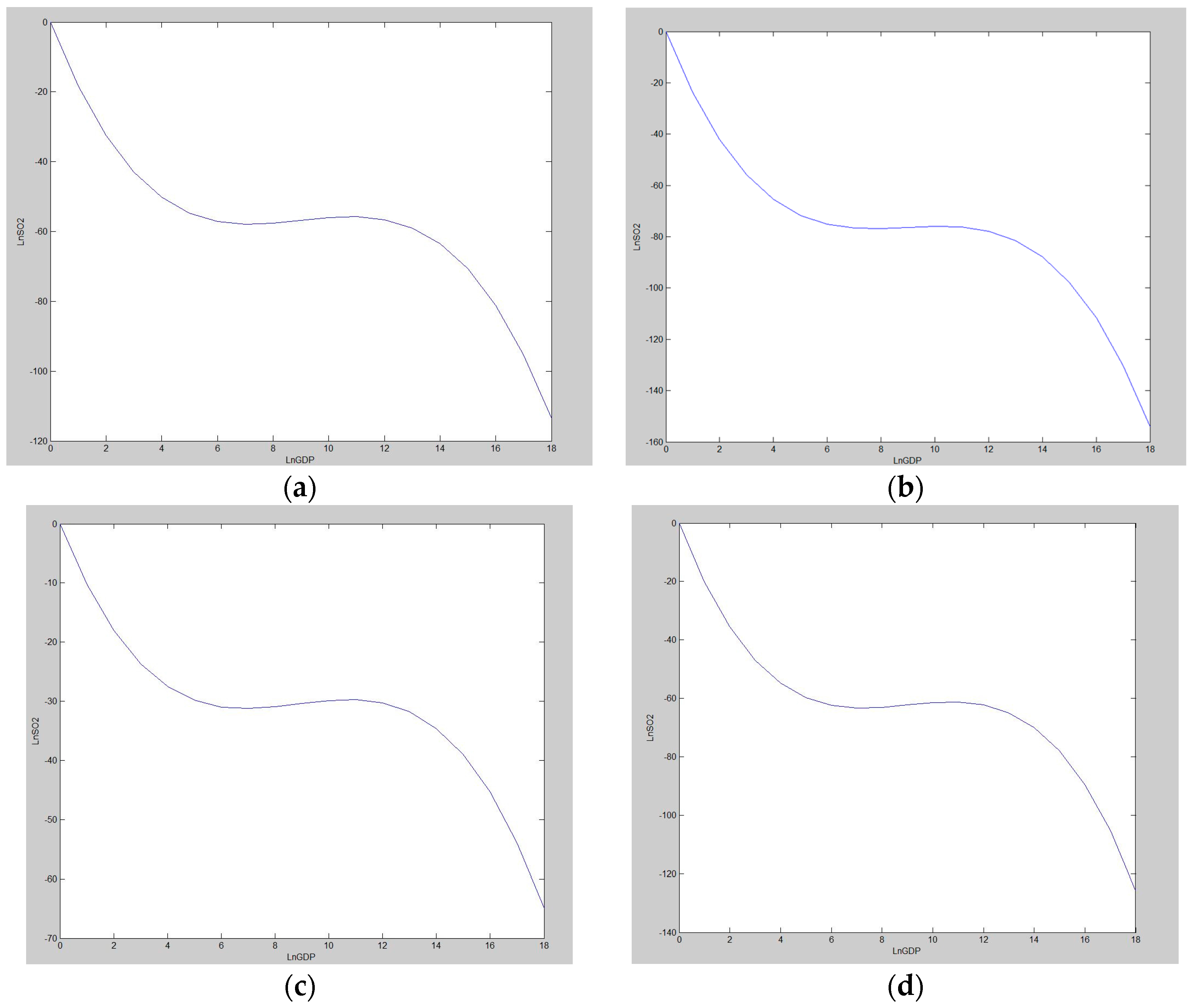To further detect the clustering pattern of SO₂ emission distribution, we illustrate the Moran’s I scatter plot in Figure 1. Four quadrants in each scatter plot denote four different classifications of spatial autocorrelation: quadrants I, II, III, and IV, refer to High–High, Low–High, Low–Low, and High–Low clustering, respectively. The slope of the line through the points reflects the clustering strength. Clearly, most of the points lie in quadrants I and II in each scatter plot, which means, in our study time period, the High–High and Low–Low clustering are the major distribution patterns of SO₂ emission in China.

To depict the spatial distribution of provincial SO₂ emission more intuitively, we show the distribution structure in different provinces from 2004 to 2014 in Figure 2. As we can see, beginning with 2004, the High–High clustering pattern mainly exists in Mid-East and Mid-West regions of China (Shanxi, Henan, Shandong, Hebei, etc.). On the other hand, the Low–Low clustering pattern mainly exists in the Western region (Qinghai and Xizang provinces). At the end of our study time-period, the High–High clustering pattern moved to Southeast region and Mid-North (Jiangxi, Fujian, Guangdong, etc.). However, the Low–Low clustering pattern remains in the same region as before.

5.2. Empirical Results and Analysis.

To explore the validity of including spatial effects in our model, we first reported the results of the traditional non-spatial model in

Table 3. Estimation results of Non-spatial models.

Dependent Variable: LnSO2	(1)	(2)	(3)	(4)
Intercept	188.8057 **
	(−2.0121)
Ln GDP	−56.0517 **	−32.8157 ***	−60.0464 **	−33.8968 ***
	(−2.0031)	(−5.1803)	(−2.1370)	(−5.6947)
Ln GDP2	5.6295 **	3.5534 ***	6.0473 **	3.7247 ***
	(2.0292)	(5.6070)	(2.1725)	(6.2825)
Ln GDP3	−0.1877 **	−0.1270 ***	−0.2020 **	−0.1334 ***
	(−2.0545)	(−6.0013)	(−2.2051)	(−6.7532)
Ln PA	−0.0562	−0.1602 ***	−0.0498	−0.1690 ***
	(−0.7156)	(−4.9698)	(−0.6332)	(−5.3501)
Ln POP	1.2545 ***	1.8309 ***	1.2443 ***	2.2187 ***
	(10.4975)	(5.1116)	(10.4124)	(6.2676)
R-squired	0.6399	0.3272	0.6429	0.3278
Rbar-squared	0.6345	0.3191	0.6387	0.3198
sigma-squared	0.6118	0.0217	0.6031	0.0186
Durbin-Watson	1.6115	1.6487	1.6333	1.825
LM Spatial Lag	0.0805	36.2105 ***	0.222	16.3689 ***
robust LM	19.3685 ***	4.9817 **	18.0224 ***	3.3182 *
spatial lag
LM spatial error	17.0987 ***	31.2328 ***	16.4298 ***	13.1058 ***
robust LM	36.3867 ***	0.004	34.2302 ***	0.0551
spatial error

Notes: The LM statistics are subject to a Chi-squared distribution of one degree of freedom. t statistics in parenthesis. ** p < 0.05; *** p < 0.01. Coloums (1)–(4) are model specifications of pool OLS, panel with spatial FE, time FE, both spatial and time FE (two-way fixed effects), respectively.

. Columns (1)–(4), respectively, show the results of different model specifications: pooled OLS, panel data model with spatial fixed effects only, panel data model with time fixed effects only, and panel data model with both spatial and time fixed effects (two-way fixed effects). As we can see, PA is the only variable that is not significant in pooled OLS and time fixed effect specification models, which means two things: no multi-collinearity exists between these explanatory variables; and the explanatory power of technology factor on SO₂ emission is sensitive to the model specification, especially when heterogeneity of spatial effects is not controlled for. Moreover, most of the null hypothesis of no spatial lagged dependent variable and no spatial autocorrelation in error term are rejected at 1% and 5% significant levels in the results of these model specifications. Provided the spatial test result in Section 5.1, we decide that the spatial panel model is necessary for further empirical analysis.

Following the routine [82], we estimated the SDM model to determine which spatial panel data model (SAR, SEM or SDM) to adopt. Given the results from the estimation of the SDM model, we can perform the LR test and Wald test that can help us to determine which model to choose.

Columns (1)–(3) of

Table 4. Estimation results of Spatial Durbin Model (SDM).

Dependent Variable: Ln SO2	(1)	(2)	(3)
Ln GDP	−21.6007 ***	−23.6790 ***	−20.7068 ***
	(−3.6377)	(−4.2438)	(−3.5550)
Ln GDP2	2.5777 ***	2.7029 ***	2.3982 ***
	(4.3261)	(4.8291)	(4.1299)
Ln GDP3	−0.0965 ***	−0.1002 ***	−0.0888 ***
	(−4.8264)	(−5.3376)	(−4.5947)
Ln PA	−0.1220 ***	−0.1159 ***	−0.1289 ***
	(−3.9054)	(−3.9367)	(−4.2638)
Ln POP	1.8941 ***	2.0074 ***	1.4646 ***
	(4.6246)	(5.2731)	(8.5881)
WLn GDP	−30.1911 **	−64.9640 ***	−47.4331 ***
	(−2.3977)	(−5.1608)	(−3.7131)
WLn GDP2	2.7921 **	6.2674 ***	4.5312 ***
	(2.1851)	(4.9408)	(3.5281)
WLn GDP3	−0.0882 **	−0.2085 ***	−0.1491 ***
	(−2.0424)	(−4.8615)	(−3.4507)
WLn PA	−0.0074	−0.2191 ***	−0.1858 ***
	(−0.1433)	(−3.8369)	(−3.3324)
WLn POP	0.5986	0.6881	0.3556
	(0.8487)	(0.9982)	(1.1204)
WLn SO2	0.5154 ***	0.3252 ***	0.3382 ***
	(9.7354)	(5.1157)	(5.4602)
ϕ			0.0425 ***
			(5.5719)
R-squared	0.9907	0.992	0.9909
Rbar-squared	0.3289	0.4695	0.5159
sigma-squared	0.0155	0.0134	0.0152
log-likelihood	214.8677	247.4839	127.3829

Notes: t statistics in parenthesis. ** p < 0.05; *** p < 0.01. Coloums (1)–(3) are model specifications of panel with spatial fixed effects, two way fixed effects and spatial fixed and time random effects, respectively.

represent estimation outcomes of the SDM model controlling for spatial fixed effects only and both spatial and time-period fixed effects and spatial random and time-period fixed effects, respectively.

Table 5. LR and Wald diagnostic tests.

Test	Chi-Square (1)	Chi-Square (2)	Chi-Square (3)
LR
Spatial lag	50.4872 ***	81.2615 ***	59.9059 ***
Spatial error	55.8793 ***	80.3813 ***	61.1045 ***
Wald
Spatial lag	60.2794 ***	92.1442 ***	69.3030 ***
Spatial error	49.1524 ***	89.1413 ***	61.9948 ***

Notes: Both Wald and LR test are subject to a Chi-square distribution with five degrees of freedom. ** p < 0.05; *** p < 0.01.

demonstrates the LR and Wald diagnostic test (the outcomes listed in Table 5 are based on the estimation outcomes of the Columns (1)–(3) in Table 4). All the Chi-square statistics of both LR and Wald are significant at the 1% level, which firmly rejects the hypothesis that the spatial Durbin model (SDM) can be simplified to the SAR or SEM model. Moreover, the Hausman specification test result (17.3767, 11 df, p < 0.1) denotes that the random effects model can only be rejected at the 10% level, but not at the 5% level. On the other hand, the estimation of the parameter ϕ, which stands for the weight of the cross-regional component of sample data, is another way to test the fixed effects against random effects specification. The random effects model should be rejected if ϕ goes to 0 [82]. As shown in Table 4, estimation of ϕ is 0.0425, significant at the 1% level. This result enhanced our decision of rejecting random effects model. The two-way fixed SDM model stands out with its relatively high adjusted R-square and the best flexibility (it controls for both cross-sectional and time-invariant effects). Therefore, the two-way fixed effects SDM model was set as the basis for all analyses and diagnostic tests hereafter.

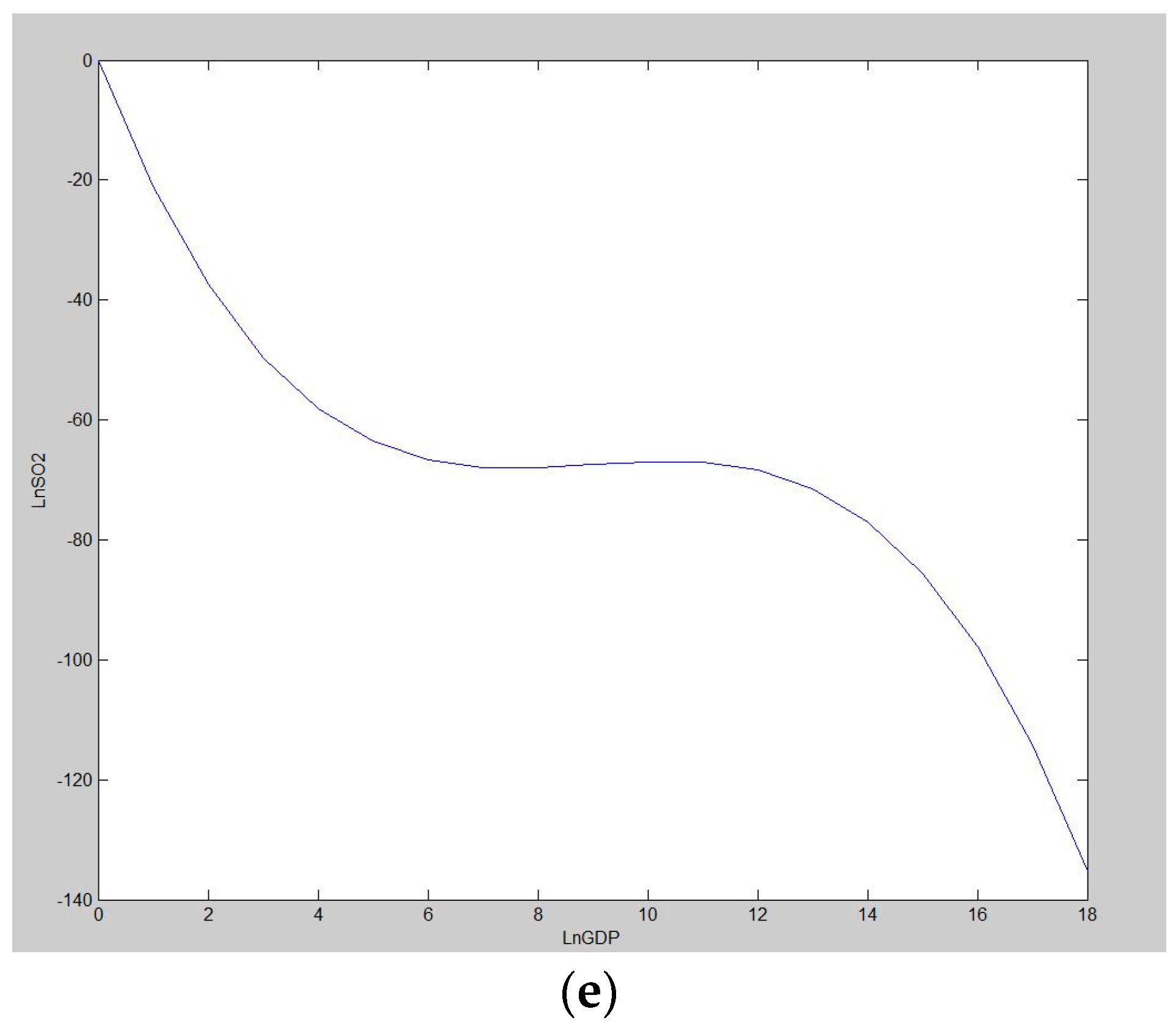
The high significance of estimated coefficients of the cubic polynomial of real GDP per capita indeed validates the assumed inverse N-shaped EKC for the SO₂ emission and economic growth nexus. This result is similar to Zheng et al. [7], Millimet et al. [48] and Kang et al. [6]. Such an inverse N-shaped environmental Kuznets Curve is displayed in Figure 3a. The two turning points based on the trajectory of EKC are approximately 1315.9 (RMB) and 50121 (RMB) (calculation of all turning points is based on different models that have control for two-way fixed effects and the calculation formula is $GDP=\exp (\frac{-2{\beta }_2\pm \sqrt{4{{\beta }_2}^2-12{\beta }_1{\beta }_3}}{2{\beta }_1})$). 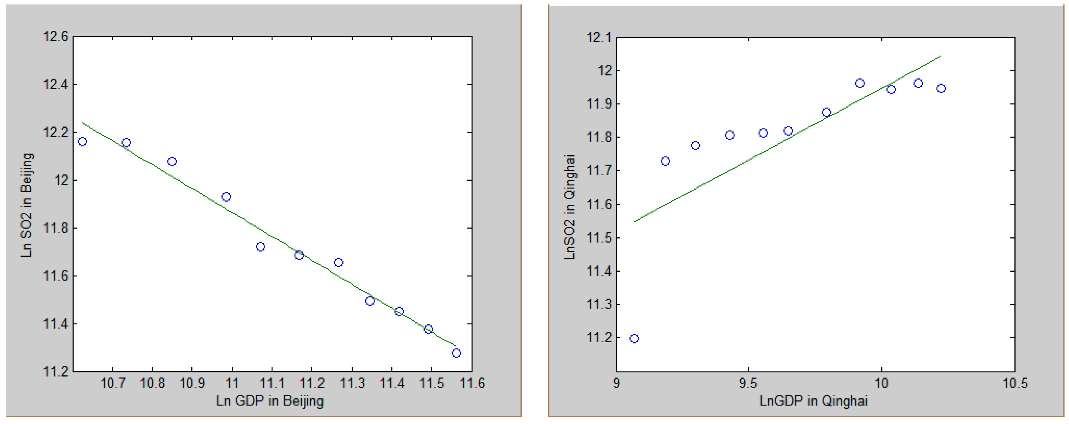According to our sample interval, the provinces are either in the upward phase (less developed regions) or the second downward phase (developed regions) in the N-shape. A typically developed region with personal income higher than 50,121 (RMB) (e.g., Beijing) is experiencing a continuous SO₂ emission decrease during the whole time span of our study. Simultaneously, the typical less developed regions with personal income between 1315.9 (RMB) and 50,121 (RMB) (e.g., Qinghai province) are experiencing an SO₂ emission increase (Figure 4).

The mechanism of such a relationship between SO₂ emission and economy can be explained by both the Chinese government’s environment preserving policy and the increase of public’s awareness on environmental preservation. More specifically, since 2006, the first year of the 11th Five-Year plan, China has conducted a series of enforcements (e.g., investments on sulfur removal devices and coal replacement in the industrial process) to limit and reduce the SO₂ emission in the second industry sector. The second industry sector in China has been the main source of SO₂ emission and the key factor for EKC (will be empirically clarified in Section 6.4). More generally, when the affluence has accumulated to a certain amount in a society, the public will eventually trade part of the economic efficiency for a better environment and living condition by means of technological, economic and political ways [73,74,84].

As mentioned before, the parameter estimates of the explanatory variables in the SAR and SDM model can be interpreted neither as the marginal (direct) effects nor as the spillover effects on the dependent variable. Instead, Equation (11) presents a correct way for calculating the direct and spillover effects. To derive Equation (11), one can multiply both sides of Equation (7) by the term ${(I-\delta W)}^{-1}$, and then Equation (11) can be easily derived. Furthermore, taking the expectation of the left-hand side of Equation (11), namely $E(Y)$, and then partial derivatives on both sides, Equation (12) can be derived. The direct and spillover effects are estimated by the partial derivatives in Equation (12). ${(I-\delta W)}^{-1}$ can be calculated by Equation (13).

$$Y_t={(I-\delta W)}^{-1}(\mu +\eta )+{(I-\delta W)}^{-1}(X_t\beta +\gamma W{X}_t)+{(I-\delta W)}^{-1}{\epsilon }_t$$

(11)

$${\left[\begin{array}{ccc}\frac{\partial E(Y)}{\partial X_{1k}}& \dots & \frac{\partial E(Y)}{\partial X_{nk}}\end{array}\right]}_t=\left[\begin{array}{ccc}\frac{\partial E(Y_1)}{\partial X_{1k}}& \dots & \frac{\partial E(Y_1)}{\partial X_{nk}}\\ ⋮& \ddots & ⋮\\ \frac{\partial E(Y_n)}{\partial X_{1k}}& \dots & \frac{\partial E(Y_n)}{\partial X_{nk}}\end{array}\right]={(I-\delta W)}^{-1}\left[\begin{array}{cccc}{\beta }_k& w_{12}{\gamma }_k& \cdots & w_{1n}{\gamma }_k\\ w_{21}{\gamma }_k& {\beta }_k& \cdots & w_{2n}{\gamma }_k\\ ⋮& ⋮& \ddots & ⋮\\ w_{n1}{\gamma }_k& w_{n2}{\gamma }_k& \cdots & {\beta }_k\end{array}\right]$$

(12)

$${(I-\delta W)}^{-1}=I+\delta W+{\delta }^2{W}^2+{\delta }^3{W}^3+\cdots$$

(13)

where $w_{ij}$ is the element on the $i$th row, and the $j$th column in matrix $W$. The diagonal elements in the partial derivatives matrix refers the direct effects (elasticity), while all the off-diagonal elements refer to spillover effects. Consequently, if it is true that both $\delta =0$ and $\gamma =0$, spillover effects do not exist, since we finally adopt the SDM model in the current research [82].

The direct and spillover effects estimate of technology advancement and population on SO₂ emission are listed in

Table 6. Direct and spillover effects estimates based on the two way fixed effects SDM model.

Variable	Direct	t-Statistic	Spillover	t-Statistic	Total	t-Statistic
The results based on Equation (2)
Ln PA	−0.1356 ***	−4.61	−0.3597 ***	−4.7545	−0.4953 ***	−5.9923
Ln POP	2.1280 ***	6.0564	1.8691 **	2.179	3.9971 ***	4.7661
The results based on Equation (3)
Ln PA	−0.1228 ***	−4.2551	−0.1842 **	−2.5153	−0.3071 ***	−3.9763
Ln POP	2.1430 ***	5.9452	1.026	1.3461	3.1689 ***	4.5189
TO	−0.0695	−0.7327	0.4546 **	2.1598	0.3851	1.4506
URBEN	−0.3047	−1.2522	−2.3475 ***	−5.1859	−2.6522 ***	−5.8456
The results based on Equation (4)
Ln PA	−0.1040 ***	−3.7294	−0.1923 ***	−3.6088	−0.2963 ***	−5.7789
Ln POP	1.0138 ***	3.0142	−1.1343	−1.8864	−0.1205	−0.2243
Coal	0.2024 ***	2.9674	0.0662	0.4579	0.2685	1.8858
Electric	0.3950 ***	4.0924	0.6829 ***	3.1579	1.0780 ***	4.8383
The results based on Equation (5)
Ln PA	−0.1335 ***	−4.6658	−0.1841 **	−2.5752	−0.31761 ***	−4.3191
Ln POP	2.2500 ***	6.9886	1.8207 **	2.3004	4.0707 ***	5.4549
Ln Sec	0.4151 **	2.7228	3.5385 ***	6.6234	3.9537 ***	6.3368
The results based on Equation (6)
Ln PA	−0.1368 ***	−4.5818	−0.3610 ***	−4.6565	−0.4979 ***	−6.1095
Ln Popd	2.1110 ***	5.9330	1.8519 **	2.1670	3.9628 ***	4.8154
The results of the model with second order rook W
Ln PA	−0.1982 ***	−6.6156	−0.0633	−0.6073	−0.2615 **	−2.3965
Ln POP	3.5228 ***	9.127	10.8479 ***	5.0518	14.3707 ***	6.3091
The results of the model with inverse distance W
Ln PA	−0.1912 ***	−6.9015	−0.8202 ***	−2.8354	−1.0114 ***	−3.4288
Ln POP	1.9340 ***	5.7269	9.8102 ***	3.3072	11.7442 ***	3.9863

Notes: ** p < 0.05; *** p < 0.01.

and all the model specifications in this table control for two-way fixed effects. Overall, the direct and spillover effects of both technology advancement and population are highly significant. Focusing on the technology advancement term, its estimated direct effects (elasticity) is −0.1356 and its coefficient estimates −0.1159 (Table 4, Column (2)), which holds that the local technical progress benefits the local SO₂ reduction and its feedback effect amounts to 15% of the direct effects. Comparing these results to its counterpart in non-spatial model results (Table 3, Column (4)) −0.1690, and we know that the elasticity is overly estimated by 25% due to the negligence of spatial dependence. Similarly, the direct effects (elasticity) of population factors appears to be 2.1280, indicating that population exerts a positive effect on SO₂ emission on a large scale, which is similar to the result of Wang et al. [3]. It was 4.2640% overestimated by the non-spatial model. Moreover, the feedback effect of the population is 0.1200, 5.660% of its direct effect. These results confirm above-mentioned beneficial effects of technology advancement on environmental improvement and theory in Ehrlich and Holdren [65]: more population, more pollution.

Now, we turn to spillover effects. They are also reported in Table 6. Lesage [8] mentioned that spillover effects refers to the impacts from a specific region that exerts on all other regions or vice versa. According to the results, a 1% increase of technology advancement in the local province will on average lead to a 0.3597% decrease of SO₂ emission in all the neighboring provinces. Conversely, a 1% increase of technical progress in all neighboring provinces will yield a 0.3597% decrease of SO₂ emission in the local province. On the other hand, the spillover impacts of population on the SO₂ emission are 1.8691. Namely, a 1% increase in the local population will averagely increase SO₂ emission in all neighboring provinces by 1.8691% and vice versa. Note that the spillover effects of dependent variable (SO₂) should still be interpreted by its coefficient estimates. The estimated coefficient of spatial autocorrelation, SO₂ emission, is 0.3252, significant at the 1% level (Table 4, Column (2)). It suggests that a 1% SO₂ emission increase in local provinces will, on average, lead to a 0.3250% increase in adjacent provinces and vice versa. The agglomeration and spillovers of technological progress found in China [85] could account for the negative technological spillover effects on SO₂ emission here. In the context of China, the technological agglomeration is more prominent than other economic activities and tend to be more clustered over time in space, and the human capital flows, externalities of R&D, competition as well as cooperation between local markets are the main causes for technological agglomeration and spillovers. The R&D and innovation in public sectors transmit through information network could not completely replace researcher exchange, seminars, field trips, paper documentation and science facilities in industrial and commercial R&D. To pursue monopoly profits, industry and firm create technological barriers in case of negative externality. Such barriers are very effective on remote competitors, but not on the neighboring ones due to convenient outflow of human capital [85]. This corresponds to the hypothesis that geographic boundaries may constrain technological spillovers [86].

The positive spillovers of population may be explained by migration effects. The improvement of environmental quality related to economic development essentially refers to resolving pollutions rather than passing them off to younger generation or people in other places. In reality, solution of pollution issue may be represented by increased capability of polluters in well-off areas to distance themselves from heavy ambient pollution caused by their own consumption and polluting activities.

Furthermore, distancing behavior consists of two aspects: relocating contaminated source [87] and moving out of areas of intensive pollution [88]. Therefore, migration could an important contributing factor behind the population spillover effects on neighbor emission. Parenthetically, groups in different communities have different ability of migrating away from polluted areas, thus the migration effects also tend to increase environmental inequality and be a driving force of EKC [28].

The total effect of a variable naturally includes both direct and spillover effects. It illustrates a complete contribution of this explanatory variable to the SO₂ emission. According to the results in Table 6, we conclude that the population has a stronger influence (in absolute value) on the SO₂ emission than the technical progress (3.9970 vs. −0.4953).

Regarding the facts in China, the effective impacts of technical progress on reduction of SO₂ emission can be explained by three aspects: increasing investment in new energy industries, the promotion of energy industrialization, and the exhaust gas emission reduction oriented technological advancement such as the end-of-pipe abatement technology [3,5]. According to the REN21 Global Status Report [89], China possesses considerable amounts of new energies such as biofuels, wind power, hydropower, and solar power. During the 12th Five-Year Plan, 2011–2015, the goal of SO₂ emission abatement is a decrease in emissions by 8% in 2015 compared to emission amount in 2010 [3].

6. Robustness Check

As discussed in Section 2, empirical results on EKC may be sensitive to model specifications and, thus far, the spatial panel data model is still not widely used in the research of the environmental Kuznets hypothesis. Therefore, it is reasonable to question its reliability with different assumptions and specifications. Besides, some scholars like to offer policy implications in their literature (e.g., [6,7,90]). One should not ignore that policy suggestions heavily rely on the robustness of applied model and the endogeneity of explanatory variables. We conducted six robustness checks for our model specifications and illustrate the results in this section. First, we checked different lag years of technology advancement to test if hysteretic effects exist. Second, we controlled for trade and urbanization factors. Third, we controlled for energy consumption factors. Fourth, we explore the industrialization effects. Fifth, we examine if population size and density are interchangeable. Sixth, we experimented with different specifications of weight matrix.

6.1. Hysteresis of Technical Progress

Some scholars hold the view that it is common for some kinds of technical innovations to take a relatively longer time to transform into practical and effective knowledge, especially in current China, a country without competitive R&D industry [2,91]. We tested the hysteretic period of the patent application from one to seven years in the model and the results are listed in

Table 7. Hysteretic effects estimates of tech progress.

Variable	Direct	t-Statistic	Spillover	t-Statistic	Total	t-Statistic
Ln PA-1	−0.0011	−0.1866	−0.0205	−1.4694	−0.0216	−1.5396
Ln PA-2	−0.0022	−0.3556	−0.0194	−1.4142	−0.0216	−1.5211
Ln PA-3	−0.0005	−0.0835	−0.0207	−1.4462	−0.0212	−1.4087
Ln PA-4	0.0142	0.4900	−0.3355 ***	−4.4886	−0.3213 ***	−3.8930
Ln PA-5	0.0709 **	2.4168	−0.3923 ***	−4.6088	−0.3214 ***	−3.3035
Ln PA-6	0.0826 ***	2.7408	−0.4214 ***	−4.9911	−0.3388 ***	−3.5359
Ln PA-7	0.0579	1.6284	−0.4786 ***	−5.0681	−0.4208 ***	−3.9408

Notes: ** p < 0.05; *** p < 0.01.

.

Row 1 to Row 7 exhibit effects estimates of technology hysteresis from one to seven years, respectively. As we can see, none of one-, two-, and three-year effects of lagged PA terms is significant. However, PA starts to show significant spillover effects on SO₂ emission from four-year lag to the end. The direct effects on SO₂ emission reduction of five- and six-year lags of PA has are statistically significant but environmentally insignificant because of its relatively small magnitude. (These two direct effects estimates are smaller than all the other effects estimates that are both environmentally/economically and statistically significant in this paper. More importantly, all the estimates of the effects values are bootstrapped so every time we run this program, we obtain slightly different values, especially on the numbers after the second decimal. Whereas, all the numbers before the second decimal of these two direct effects are zeros. Thus, we consider its direct effects to be too small (in absolute value) to be different from zero.) Empirical analysis should not only focus on the parameters’ statistical significance and their seemingly correct signs; instead, one should also pay attention to substantive significance since statistical significance alone cannot make sense and the measurement is one of the cores in empirical studies [92,93,94,95]. In conclusion, not only are the current technical innovations beneficial to the SO₂ pollution, some technology stocks in early years can still be effective to current SO₂ emission reduction in neighboring regions. The mechanism might be that the technologies such as the end-of-pipe abatement and replacement of high SO₂ emission energies by newly developed low SO₂ emission energies can immediately reduce the volume of SO₂ emission. Similarly, the development of new energies and the promotion of energy industrialization is not a prompt process and may need time to fit in the energy market gradually.

The coefficient estimates of income, its quadratic and cubic terms in the models incorporating four-, five-, six-, and seven-year hysteretic impacts of technical progress are illustrated in

Table 8. Coefficient estimates of GDP terms and other statistics.

	(1)	(2)	(3)	(4)
The Results of Models Incorporating Tech Hysteresis
Ln GDP	−24.2123 ***	−24.6422 ***	−27.2087 ***	−28.7327 ***
	(−4.2157)	(−4.4117)	(−4.8956)	(−5.0534)
Ln GDP2	2.7601 ***	2.8372 ***	3.1117 ***	3.2723 ***
	(4.7992)	(5.0701)	(5.5794)	(5.7165)
Ln GDP3	−0.1028 ***	−0.1064 ***	−0.1160 ***	−0.1215 ***
	(−5.3357)	(−5.6686)	(−6.1931)	(−6.2967)
R-squared	0.9916	0.992	0.9921	0.9919
Rbar-squared	0.4163	0.4258	0.4389	0.4436
log-likelihood	236.6529	243.9307	246.9031	243.6172
Observations	341	341	341	341
The Results of Models in Section 6.2, Section 6.3, Section 6.4 and Section 6.5
Ln GDP	−26.6920 ***	−11.5324 **	−22.6579 ***	−23.7406 ***
	(−4.6778)	(−2.1765)	(−4.2545)	(−4.2525)
Ln GDP2	3.0372 ***	1.3725 ***	2.6276 ***	2.7084 ***
	(5.2901)	(2.5494)	(4.8814)	(4.8362)
Ln GDP3	−0.1128 ***	−0.0517 ***	−0.0976 ***	−0.1004 ***
	(−5.8420)	(−2.8444)	(−5.3787)	(−5.3439)
R-squared	0.9928	0.9875	0.9930	0.9920
Rbar-squared	0.5365	0.5074	0.5459	0.4694
log-likelihood	267.2332	298.8698	271.7530	247.4841
Observations	341	330	341	341

Note: t statistics in parenthesis. ** p < 0.05; *** p < 0.01. In tech hysteresis part, results in Columns (1)–(4) refer to models with four-year lag to seven-year lag of technical progress respectively. In the Section 6.2, Section 6.3, Section 6.4 and Section 6.5 part, results in Columns (1)–(4) refer to models incorporating socio-economic factors, energy consumptions, industrial composition, population intensity, second order rook W and inverse distance based W respectively. All the models are panel with two-way fixed effects.

. They all are significant at the 1% level and keep the same signs as before, which means that the inverse N-shape nexus of SO₂ emission and income is still water tight.

6.2. Socio-Economic Activities

In 2001, China joined the WTO, which boosted its export and import markets. According to the pollution haven hypothesis, wealthy countries tend to export their pollutions to less developed countries. Chinese government has been conducting urbanization as one of the economic policies and expanding the cities on a large scale for decades. Other than that, trade openness [6,96,97] and urbanization [5,98] were found significantly related to environmental impacts and exhausted gas emission. Therefore, it is necessary to see if our basic conclusion stays unchanged when controlling for these two economic factors.

As we can see in Table 6 (results based on Equation (3)), both effects of technical progress remain significant and negative. However, the spillover effects of technical progress shrank significantly, from −0.3597 to −0.1842, and, thus, its total effects shrank as well, from −0.4953 to −0.3071. On the other hand, only a slight change occurs in the direct effect of population, while its spillover effects are no longer significant. Although we do not focus on the trade and population effects in the current paper, the increased adjusted R square (Table 8, Column (2)) and significant spillover effects of trade openness and urbanization terms indicate that their inclusion would enhance the model’s explanatory power.

Moreover, the positive indirect effects of trade openness is in consistence with PHH, indicating that the regions with higher level of openness and loosen environmental regulations tend to attract less environmental-friendly foreign firms. The negative urbanization elasticity of SO₂ emission is probably not the result of economies of scale on public infrastructure, since currently in China, a big development gap exists between urban and rural areas and shortages of basic public services are still in many rural areas. Instead, such negative indirect effects may be induced by the urbanization’s beneficial impacts mentioned in Section 3.2, especially the effects of advanced approach to modernized means of energy utilization, which is proposed by Pachauri [99] as well as Pachauri and Jiang [100]. They argued that replacement of inefficient solid fuels by modern and advanced energy utilization ways enables residents and industries in urban areas reduce energy consumption to a lower level than that in rural areas.

6.3. Energy Consumption

Energy consumption is always a factor that was taken into account by many scholars in the studies of air pollution [2,3,6,90]. The coal combustion is one of the major sources of SO₂ emission. Besides, electricity consumption is also considered as the main contributor to SO₂ emission in China [101]. We tested the model controlling for coal and electricity consumptions with a reduced sample size since these data are not available in Tibet province. Table 6 (results based on Equation (4)) depicts the results. As is shown, similar to the results of controlling for trade openness and urbanization, the sigh of the direct and spillover effects of technical advancement is still negative. This means technical progress is still significantly beneficial to the emission abatement after controlling for energy consumption factors, whereas the amounts of all the direct, spillover, and total effects of technical progress decreased again. As for the population term, its spillover effects became less significant and negative. Electricity consumption has significant positive effects on SO₂ emission, which corresponds to China’s heavy reliance on thermal power generation and is in line with the results in Lu et al. [101].

6.4. Industrial Composition

As discussed in Section 3.2, industrialization level represented by SEC-GDP ratio is another key factor for ambient pollution. Environmental quality may change as the outflow from the traditional secondary industry to non-energy/pollution-intensive service industry occurs. The results of controlling for SEC-GDP ratio arelisted in Table 6 (results based on Equation (5)). The expected positive and highly significant parameters of SEC-GDP ratio suggests that higher share of secondary industry added to GDP increase SO₂ emission because most energy and emission intensive sectors lies in the secondary industry. According to National Statistics Bureau of China, most developed cities/provinces experienced decreases in share of secondary industry while less developed areas went through first an increase and later a decrease during 2004–2014, which may be the result of China’s recent implementation of Industrial Upgrading Reform.

These findings are in line with the mechanism stated in Syrquin and Chenery [102], Suri and Chapman [81], Stern [80] and Dinda [28]: SEC-GDP ratio increase in the early stage for the pursuit of industrialization, then decrease as the structure changes for higher efficiency and lower emission. Besides, the magnitudes in estimates of technical progress and population impacts only change slightly and stay highly significant. This shows us the inclusion of SEC-GDP ratio captures other effects omitted by other independent variables, which improves the model’s explanatory power and makes our conclusion on SEC-GDP ratio more pronounced. Importantly, the variation of SEC-GDP ratio is generally parallel to the fluctuation of SO₂ emission, plus the ration and emission are statistically positive associated, thus we argue that the SEC-GDP ratio is an important driving force of the SO₂ EKC.

6.5. Population Density

Significant and positive estimates of direct and spillover effects of population density (Table 6) suggest the noticeable impacts of population density on local and neighbor areas. More specifically, they are close to the population effects (in results of Equation (2)) in amount (direct: 2.1110 vs. 2.1280; spillover: 1.8519 vs. 1.8691), implying population and population density may be interchangeable proxies in study of China’s emissions. The still significant and slightly changed direct and spillover effects of technical progress also support this view.

The reason behind this is probably in China, areas with more people generally have higher population density. For example, fewer people live in four largest provinces, Xinjiang, Tibet, Inner Mongolia and Qinghai, while Jiangsu, Hebei and Henan, considerably smaller in area, have more residents.

6.6. Spatial Weight Matrix Specifications

Although the application of a “standard” first order contiguity spatial weight matrix is the most popular specification in the prior literature, an alternative spatial weight matrix specification applied in spatial models might be reasonable and can result in different outcomes. We experimented other two normally used spatial weight matrix specifications: second order rook contiguity (in the context of China, the spatial weight matrix of rook contiguity is the same with the matrix of queen contiguity; therefore, it is only necessary for us to test either spatial weight matrix specification or these two) and inverse distance based (the distance is measured by Euclidean distance between the centroid of different regions) matrix to examine the stability of prior basic results.

Table 6 also presents the effects estimate with both weight matrix specifications. In both specifications, direct and spillover effects estimates of technical progress are highly significant at 1% level, except for its spillover effects in the second-order specification. On the other hand, the spillover effects estimates of population (10.8479; 9.8102) in both specifications blow up six times (or more) the magnitudes of their counterparts in all other models, which is rather unreasonable and also inconsistent with results in prior studies on similar themes (e.g., Kang et al. [66], and Sinha and Bhattacharya [103]). These results are doubtful. Thus, we tentatively put forward that these two weight matrices specifications are inadequate for describing the population impacts on SO₂ emission in neighbor provinces. This is probably due to the reason that more neighbor spatial units are taken into account since these two specifications pre-assumed that population spillover pass through the first order neighbors and travel to higher order ones. However, the mechanism behind the diffusion of population effects on environmental impacts is not discussed in prior studies, although this is not our concern in the current study. Therefore we will not continue the discussion of results from these two specifications in the following part.

All the coefficient estimates of income, and their quadratic and cubic terms for the four different models in Section 6.2, Section 6.3, Section 6.4 and Section 6.5 are reported in Table 8. It should be noted that the coefficients estimate of income and its quadratic as well as cubic terms diminished by half in the model that controls for energy factors (Table 8, Column (2)). This is probably caused by the reduced sample size. The signs of coefficients stay unchanged and they are still significant at the 5% or 1% levels. This indicates that inversely N-shaped EKCs can basically reflect nexus of emission and economic growth under different model specifications. However, features of the shapes varies in details (Figure 3) and turning points are quite sensitive (

Table 9. EKC estimation.

Estimation Model	First Derivative	Turning Points
$\ln S{O}_2=-20.7068\ln GDP+2.3982(\ln GDP{)}^2-0.0888{(\ln GDP)}^3$	$-20.7068+4.7964\ln GDP-0.2664{(\ln GDP)}^2$	1315.9; 50121
$\ln S{O}_2=-26.6920\ln GDP+3.0372(\ln GDP{)}^2-0.1128{(\ln GDP)}^3$	$-26.6920+6.0744\ln GDP-0.3384{(\ln GDP)}^2$	2165.3; 28857
$\ln S{O}_2=-11.5324\ln GDP+1.3725(\ln GDP{)}^2-0.0518{(\ln GDP)}^3$	$-11.5324+2.745\ln GDP-0.1554{(\ln GDP)}^2$	976.72; 48045
$\ln S{O}_2=-22.6579\ln GDP+2.6276(\ln GDP{)}^2-0.0976{(\ln GDP)}^3$	$-22.6579+5.2552\ln GDP-0.2928{(\ln GDP)}^2$	1338.4; 46574
$\ln S{O}_2=-23.7406\ln GDP+2.7084(\ln GDP{)}^2-0.1004{(\ln GDP)}^3$	$-23.7406+5.4096\ln GDP-0.3012{(\ln GDP)}^2$	2073.5; 30430

Note: The parameter estimates in Row 1 to Row 5 are the results of Equations (2)–(6) listed in Table 4 and Table 8.

) to specifications and sample size, which agrees with the past studies [12,15,30]. According to our observation, personal income in all areas are greater than the first turning points (the lowest GDP per capita (4317 RMB) is in Guizhou province, 2004, greater than the maximum estimate of first turning point (2165.3 RMB)) while per capita GDP in a few developed provinces/cities (e.g., Beijing, Tianjin, Shanghai, Jiangsu and Zhejiang) surely exceed the second turning point (50,121 RMB) at the end of the period and these areas are going through declines in SO₂ emissions.

7. Conclusions and Discussions

Thus far, spatial panel data model is still not widely used in the research of environment Kuznets curve hypothesis. With the introduction of the SDM model incorporating spatial dependence, this study empirically verified the inverse N-shaped EKC hypothesis and technical progress’s beneficial direct, spillover and hysteresis effects on SO₂ reduction in China. Population size, migration effects, industrialization level and power consumption are found to be the contributing factors on increasing SO₂ emission. The present study utilized the dataset of a provincial panel of China from 2004 to 2014.

Due to the inclusion of spatial dependence of variables, the findings in this paper are more persuasive than results from traditional panel data approaches. Instead of interpreting the direct and spillover effects of explanatory variables by their coefficient estimates, we estimated both effects of the explanatory variables through the partial derivatives of equivalently transformed spatial Durbin model, which is more accurate and valid than prior studies in EKC hypothesis. Besides, according to the robustness checks, the SDM model specification in current research and its conclusions about the inverse N-shaped EKC and technical progress’s impacts show a solid stability.

According to the empirical results, the spillover effects in SO₂ emissions that are detected might be caused by the regional agglomeration of socio-economic activities and population distribution. In another way, the spillover effects can occur due to the “demonstration effects” that take place if local environmental and/or economic policies are imitated and followed by neighbors and vice versa. In China, the central government draws up the overall national plan of economic growth and pollutants emission abatement each year, then decomposes the plans at the provincial and city levels. Achievements in economic growth and pollutant emission control are evaluated in provinces and cities and they are highly related to the local officials’ careers. Such a local government evaluation system gives incentives for competition and imitation among provinces and cities in terms of pollution control as well as economic development. If a local government implements rigorous controls on air pollution, the adjacent provinces may follow and implement similar ways to reduce emissions. On the contrary, if the local area still has a series of loose regulations on the environmental protection and take economic growth as the primary goal regardless of air pollution, its neighbors would probably implement a similar strategy to catch up in terms of economic development [4]. The mimic behaviors among local governments can simplify their policymaking and prevent new policies adding extra costs and risks. Geographic characteristics and such “demonstration effects” may account for the significant spatial effects of socio-economic, energy consumption and industrial composition factors. For example, clustering of heavy industries in northeast old industrial area, agglomerations of manufacturing industries and booming international trade markets in southeast coast, are possibly induced by economic policies, exemplary role of wealthy areas and geographical factors.

From the general trend, SO₂ emission in developing provinces will first experience an increase and then a decrease with China’s continuous economic growth and the emissions in developed provinces will keep decreasing. A clean environment becomes more demanded as income levels improve. Although the economic growth enable us to invest more on the pollution control and the R&D for the pollutants abatements, we cannot simply wait to reach the turning point in those less developed regions: the thresholds of total SO₂ must not be exceeded, otherwise the environmental system can no longer withhold the pollution. From the provincial perspective, the SO₂ emission and its determinants have significant spillover effects on local and adjacent areas. This implies that the policymakers of central government need to make overall plans for emission reduction based on the development, technology and industry characteristics in different provinces. The administrative boundaries should be broke for local government cooperation on emission abatement and economic growth. Provincial level government should also keep assessments of neighbor province’s SO₂ emission to adjust the local investment on pollution treatment.

In this study, we focus on the beneficial effects that the technical advancement has on the environmental governance. However, this should not be forgotten: theoretically, technology usually possesses two-sided effect, i.e. technical progress can help us reduce the pollution and ameliorate the environmental impact while technical impacts brought by new technologies may shift the prior impact. For instance, nuclear power technology replaces thermal power plant and reduces coal consumption while increases nuclear waste and the risk of nuclear leakage. Similarly, the recently prevalent electric vehicles can shift part of the environmental burden of automobile exhaust to nearby power plants. The result in Section 6.1 shows that the technology stock takes too much time to convert into the technical improvements and finally to promote the SO₂ emission reduction. Thus, improvement of the technical conversion efficiency should be made so that the conversion period can be shortened which can further benefit on the abatement of SO₂ emission. To achieve that, R&D can optimize the distribution of research funding and cut those less effective ones.

As the effective instrumental variables for the explanatory variables are not available, and our sample data did not generate from natural experiments, it is difficult to tell whether the explanatory variables are endogenous. Since we did not apply a dynamic model, the data generating process is not yet known (the weak and super exogeneity issue). In this case, the invariance of the coefficient estimates is not discussed. Without evidence of the invariant characters of coefficient estimates, one cannot make sure that these estimates do not change when data generation process varies. Coefficients in econometric models are usually conditional on policies variance and other unobservable factors. They may vary as policies change [104,105].

Constrained by our sample interval, the mechanism of the first downward trend in the inverse N-shaped trajectory remains unclear. The relatively small values of adjusted R-squares in the results indicate that some essential driving forces other than industrial structure might be omitted in this research. The population’s spillover estimates can blow up considerably due to the different specification of the spatial weight matrix, which is possibly unrealistic; however, this is not our main concern within this research.

Further research is expected to use dynamic spatial panel data model with longer period of data to estimate the long term effects (the values the system eventually converges to) of SO₂ emission’s determinants. Discussions and studies of whether these determinants are endogenous would offer evidence for the validity of their estimates. Besides, the study on the selection of optimal specification of spatial weight matrix will be helpful for capturing the spillover effects in the EKC research. In addition, a sample with lower income and different variables are necessary for further verification and examination of the mechanism behind the first downward phase in the inverse N-shaped EKC.