Identification of Critical Factors for Non-Recurrent Congestion Induced by Urban Freeway Crashes and Its Mitigating Strategies

Abstract

Given the extreme difficulty of estimating crash likelihoods, the most important aspect of the development of congestion management strategies is the identification of the factors that affect non-recurrent congestion caused by crashes. Such factors must be identified to develop crash management strategies and congestion management strategies. The objectives of this study are to identify causal factors that affect non-recurrent congestion and to propose some operational strategies for mitigating crash-induced non-recurrent traffic congestion. To achieve these objectives, a case study was conducted to identify spatiotemporal non-recurrent congestion regions using a previously developed method based on historical inductance loop detector data collected from six major freeways in Orange County, California. Based on the case study results, potentially significant factors in non-recurrent congestion were identified using the Cox proportional hazard model. Additionally, with the factors identified as significant, operational strategies were proposed for mitigating non-recurrent congestion due to freeway crashes.

1. Introduction

Although it has been speculated that non-recurrent congestion caused by incidents such as crashes, disabled vehicles, spills, weather events, and visual distractions accounts for one half to three fourths of the total congestion on metropolitan freeways [1,2], there are insufficient data to either confirm or deny this conjecture. In addition, there is limited information available on how to allocate resources in an effective way to mitigate non-recurrent congestion caused by freeway incidents. Specifically, given the extreme difficulty of estimating crash likelihoods, because of the nature of non-recurring congestion, the most important aspect of the development of congestion management strategies is the identification of the factors that affect non-recurrent congestion caused by crashes. This requires basic information on how, where, and to what extent congestion occurs. Effective congestion management requires that traffic operators have a full understanding of how traffic congestion is affected by crashes.

The spatiotemporally negative impact (i.e., non-recurrent traffic congestion) of crashes has been examined in various recent studies (e.g., [3,4,5,6]). However, most of these studies were focused on developing methods for identifying spatiotemporal crash regions. Chung and Recker [3] presented an approach to quantifying non-recurrent congestion in terms of total delays through spatiotemporal crash impact regions, as well as a relationship between the total delay and the factors that affect it, based on univariate analysis. Since this type of analysis describes the total delay with respect to each factor individually, it does not adequately describe the combined effect of the significant factors. The objectives of this study are therefore to identify the causal factors that affect non-recurrent congestion and to propose some operational strategies for mitigating crash-induced non-recurrent traffic congestion. To achieve these objectives, the method by Chung and Recker [3] was used to identify regions of non-recurrent traffic congestion caused by crashes in Orange County, California, and Cox’s semi-parametric model was used to analyze the results and assess the effect of multiple variables on non-recurrent congestion caused by urban freeway crashes.

2. Literature Review

2.1. Overview of Identification of Spatiotemporal Traffic Congestion Impact

Before the factors that cause congestion induced by traffic crash can be identified, traffic congestion must be quantified. Several approaches to assessing the spatiotemporally negative impact (i.e., non-recurrent traffic congestion) of crashes have been proposed. The methods proposed for analyzing traffic flow data obtained from the field can be classified in the following three categories: (1) methods that use deterministic queuing diagrams (e.g., [7,8,9,10,11,12,13]), (2) methods that use kinematic wave theory (e.g., [14,15,16,17,18,19,20]), and (3) empirical methods (e.g., [3,4,5,6,21,22,23]). Although any of these three types of methods can be applied for purpose such as those of this study, only a few studies have demonstrated how to estimate non-recurrent congestion based on field data such as ubiquitous loop detector data [3,23].

Chung and Recker [3] proposed an approach to distinguishing the non-recurrent congestion from recurrent congestion at the time and place of a reported crash for the purpose of estimating the contribution of non-recurrent congestion caused by the specific crash. The approach proposed by Chung and Recker was taken in this study to identify non-recurrent congestion due to individual traffic crashes. The results were used in the identification of critical factors based on multivariate statistical analysis.

2.2. Identification of Spatiotemporal Congestion Impact Induced by Crashes

Chung and Recker [3] proposed an approach to capturing spatiotemporal congestion based on crash information, road traffic information, and roadway facility information. The method is based on the assumption that traffic flow has spatiotemporal patterns under the normal flow conditions if no special events, such as crashes, occur. However, once a crash occurs, it has a negative impact on traffic flow (i.e., a speed drop). Although Chung and Recker assumed that traffic flow may have a specific pattern with respect to space and time, traffic on a roadway typically fluctuates even under normal flow conditions. Such fluctuations are taken into consideration in the method using the annual average speed and standard deviation for each roadway section and five-minute time period. Using traffic flow data collected over the course of one year and these basic statistics, a discrimination function is developed to distinguish between a speed drop (or crash speed) induced by a crash and one (or a crash-free speed) induced by normal traffic fluctuation for each time period and roadway section. Finally, spatiotemporal congestion impact regions resulting from crashes are estimated using binary integer programming (BIP) to distinguish regions in which the traffic speeds are affected by crashes from those in which they are not. This method consists of the following three steps:

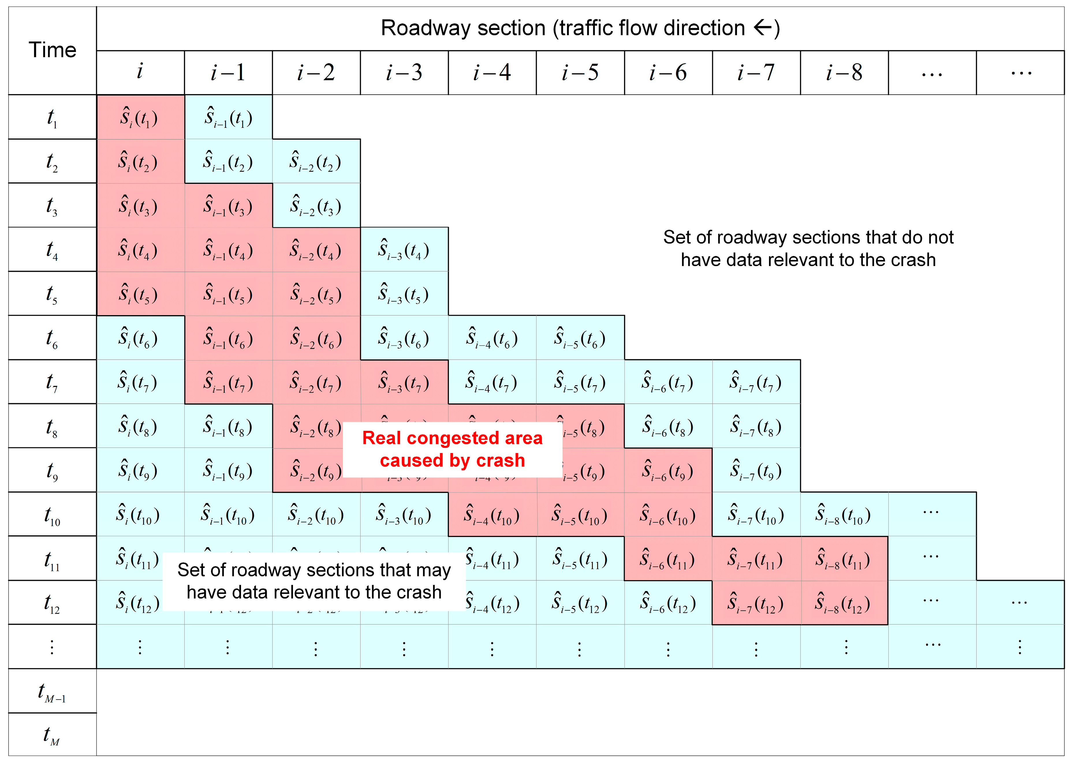
2.2.1. Step 1: Data Arrangement

The first step in this method is to arrange the traffic flow data. Two datasets are required: a set of traffic flow data (speeds and volumes) with respect to time and space (or by roadway section) and a set of crash data, including crash times and locations. For each roadway section $i$ and each specific time interval $t_m$ on each day of the week, a nominal total of $R$ speed ($s_i(t_m)$) and volume ($q_i(t_m)$) observations are available during the observation period. If a traffic flow dataset collected over the course of one year is used, then during a specific time interval for a given day of the week there are 52 speed samples (i.e., $R=52$) for section $i$. The nth speed for any particular combination of the day of the week, time interval, and section can be expressed as $s_{in}(t_m)$.

Using the collected speed data, the average speed ${\overline{s}}_i(t_m)$ and its standard deviation ${\sigma }_{s_i\left(t_m\right)}$ for section $i$ and time interval $t_m$ under crash-free conditions are determined. Then, for $t_m>t_o,m=1,2,\cdots$ (i.e., time intervals after the occurrence of a crash in section $i$ at time $t_o$), a series of average speeds and standard deviations can be composed as $\left\{{\overline{s}}_i(t_1),{\sigma }_{s_i\left(t_1\right)}\right\}$, $\left\{{\overline{s}}_i(t_2),{\sigma }_{s_i\left(t_2\right)}\right\}$, $\left\{{\overline{s}}_i(t_3),{\sigma }_{s_i\left(t_3\right)}\right\}$,$\cdots$

The crash dataset collected for the same time period and for the same roadway coverage is used. If a crash occurs in section $i$ during time interval $t_1$, all upstream sections could possibly be affected by the crash. The corresponding speeds ${\widehat{s}}_i(t_m)$ and volumes ${\widehat{q}}_i(t_m)$ can be presented in matrix form as shown in

Table 1. Arrangement of crash-related traffic flow data in matrix form.

Time	Roadway Section (Traffic Flow Direction ←)
	$\mathit{i}$	$\mathit{i}-1$	$\mathit{i}-2$	$\cdots$
$t_1$	$\left\{s_i(t_1),q_i(t_1)\right\}$	$\left\{s_{i-1}(t_1),q_{i-1}(t_1)\right\}$	$\cdots$	$\cdots$
$t_2$	$\left\{s_i(t_2),q_i(t_2)\right\}$	$\left\{s_{i-1}(t_2),q_{i-1}(t_2)\right\}$	$\cdots$	$\cdots$
$⋮$	$⋮$	$⋮$	$⋮$	$⋮$
$t_m$	$\left\{s_i(t_m),q_i(t_m)\right\}$	$\left\{s_{i-1}(t_m),q_{i-1}(t_m)\right\}$	$\cdots$	$\cdots$
$⋮$	$⋮$	$⋮$	$⋮$	$⋮$
$t_{M-1}$	$\left\{s_i(t_{M-1}),q_i(t_{M-1})\right\}$	$\left\{s_{i-1}(t_{M-1}),q_{i-1}(t_{M-1})\right\}$	$\cdots$	$\cdots$
$t_M$	$\left\{s_i(t_M),q_i(t_M)\right\}$	$\left\{s_{i-1}(t_M),q_{i-1}(t_M)\right\}$	$\cdots$	$\cdots$

.

2.2.2. Step 2: Establishment of Maximum Crash Impact Region

The second step is to establish the maximum possible extent of the crash impact. This step is performed to reduce the computation load. The maximum possible extent is established for the worst possible conditions (i.e., total blockage). For any given crash occurring in the roadway section $i$ during time interval $t_1$, we compute the maximum number of upstream sections that could be affected by the assumed persistent total blockage in section $i$ during time interval $t_1$. Using this spatiotemporal information, the “maximum area of interest” for any crash occurring in section $i$ during time interval $t_1$ can be constructed schematically based on the speed and volume matrix composed in the first step. As a result, a portion of the speed and volume data matrix illustrated in Table 1 is not included in the maximum crash impact region. Only some of the spatiotemporal areas in the schematically constructed speed matrix are related to truly congested areas resulting from the crash. Figure 1 shows the maximum set and real set of roadway sections affected by the crash. This figure consists of three sets of spatiotemporal speeds: the set of roadway sections that do not have data relevant to the crash, the set of roadway sections that may have data relevant to the crash, and the set of roadway sections that have data relevant to the crash.

2.2.3. Step 3: Construction of Crash Impact Region

The third step is to construct the real crash impact region from the maximum crash impact region. Since the speed of traffic in sections adversely affected by a crash is reduced, these two regions can be distinguished by comparing the crash-affected speed ${\widehat{s}}_j(t_m)$ to the distribution of the crash-free speeds $s_{jn}(t_m)$ and assigning some level of confidence that any particular ${\widehat{s}}_j(t_m)$ was not drawn from the distribution of $s_{jn}(t_m)$. Binary integer programming (BIP) is used in the following manner to distinguish between speeds that are and are not affected by a crash:

$$\begin{array}{ll}\underset{{\delta }_{jm}}{Min}& Z={\displaystyle \sum _{\forall j,m}\left[P_{jm}\cdot {\delta }_{jm}+(1-P_{jm})\cdot (1-{\delta }_{jm})\right]}\\ & \\ \mathrm{s}.\mathrm{t}:& \\ & \\ & {\delta }_{j+k,m}\le \left[1-({\delta }_{j,m}-{\delta }_{j+1,m})\right]\cdot G;\forall j,m;\forall k\le J-j\\ & {\delta }_{j,m+r}\le \left[1-({\delta }_{j,m}-{\delta }_{j,m+1})\right]\cdot G;\forall j,m;\forall r\le M-m\\ & {\delta }_{j,m+k}\le \left[1+({\delta }_{j,m}-{\delta }_{j+1,m})\right]\cdot G;\forall j,m;\forall k\le M-m\\ & {\delta }_{jm}=\{\begin{array}{ll}0\hfill & \hfill \\ 1\hfill & \hfill \end{array}\end{array}$$

(1)

where $\delta$ is a binary variable, $G$ is an arbitrarily assigned large number (e.g., one million), $J$ is the maximum number of upstream sections, and $M$ is the maximum number of subinterval time periods (e.g., for five-minute subintervals and a maximum analysis time period of 4 h, $M=48$). The value of the decision variable $P_{jm}$ used to distinguish between affected and unaffected speeds is calculated as follows:

$$P_{jm}=\{\begin{array}{lll}0;\hfill & {\widehat{s}}_j(t_m)\le {\overline{s}}_j(t_m)-0.25{\sigma }_{s_j(t_m)}\hfill & ;n_{obs}\ge 30\hfill \\ 1;\hfill & {\widehat{s}}_j(t_m)>{\overline{s}}_j(t_m)-0.25{\sigma }_{s_j(t_m)}\hfill & ;n_{obs}\ge 30\hfill \\ 0.5;\hfill & \hfill & ;n_{obs}<30\hfill \end{array}$$

(2)

where ${\widehat{s}}_j(t_m)$ is any speed not drawn from the distribution of $s_{jn}(t_m)$, ${\overline{s}}_j\left(t_m\right)$ and ${\sigma }_{s_j}{}_{(t_m)}$ are the average speed and standard deviation of speeds drawn from the distribution of $s_{jn}(t_m)$.

2.3. Multivariate Statistical Analysis

2.3.1. Survival Analysis

Both recurrent and non-recurrent traffic congestions are cleared with the passage of time. Such phenomena are similar to the functioning and failure of a machine or the birth and death of a living organism. Various multivariate statistical analysis methods offer a means to examine and model the time it takes for events to occur. Survival analysis, also called failure time data analysis or event history analysis, is the analysis of random variables with positive values and censored observations, such as the lifetimes of humans or other living organisms, the failure times of machine components, and the occurrence of events. However, survival analysis can be applied to a wide variety of random variables beyond those strictly representing the end of life or failure of a machine. Applications in the transportation area include, for example, the occurrence of traffic crashes [24,25], incident duration [26,27,28,29,30], households’ vehicle ownership duration [31,32,33,34], and traffic congestion [3,23,35,36,37,38].

The mathematical expression of survival analysis begins by defining a continuous random variable, $T$, denoting the “lifetime” of a subject or duration of an event. The possible values of a random variable $T$ have a probability distribution that is characterized by a probability density function (pdf), $f(t)$, and a cumulative distribution function (cdf), $F(t)$, which is called the failure function. The distribution function of $T$ is expressed as follows:

$$F\left(t\right)={\displaystyle {\int }_0^{t}f\left(u\right)du}=\mathrm{Pr}\left(T\le t\right),\cdots 0<t<\infty$$

(3)

which gives the probability that a survival time $T$ is less than or equal to some value $t$. For all points for which $F(t)$ is differentiable, a density function $f(t)$ is defined as follows:

$$f\left(t\right)=\frac{\partial F\left(t\right)}{\partial t}=\underset{\Delta t\to 0}{\lim }\frac{F\left(t+\Delta t\right)-F\left(t\right)}{\Delta t}$$

(4)

This function gives the unconditional failure rate of event occurrences in an infinitesimally small differentiable area. By expressing $f(t)$ in terms of probability, it can be written as follows:

$$f\left(t\right)=\underset{\Delta t\to 0}{\lim }\frac{P\left(t\le T<t+\Delta t\right)}{\Delta t}$$

(5)

where this function gives the instantaneous probability that an event will end (or a unit will fail) in the infinitesimally small interval $[t,t+\Delta t]$. Another important concept in survival analysis is the survivor function, $S(t)$, which is expressed as follows:

$$S\left(t\right)=1-F(t)=\mathrm{Pr}\left(T\ge t\right)$$

(6)

Having mathematically defined the survivor function and the density of end (or failure) times, the relationship between failure times and the survivor function is captured through the hazard function, $h(t)$, which is expressed as follows:

$$h\left(t\right)=\frac{f(t)}{S(t)}$$

(7)

The hazard function gives the rate at which units fail by $t$ given that the unit had survived until $t$. Therefore, it is conditional failure rate, and it can be expressed as follows:

$$h\left(t\right)=\underset{\Delta t\to 0}{\lim }\frac{\mathrm{Pr}\left(t\le T\le t+\Delta t|T\ge t\right)}{\Delta t}$$

(8)

Since this function denotes the rate of failure per time unit in the interval $[t,t+\Delta t]$, conditional on the survival time $t$, it is also often known as the hazard rate. This rate may increase, decrease, remain constant, and/or follow a more complicated process. The rate can also exhibit a variety of trends, such as an increase and subsequent decrease, or a decrease and subsequent increase over time. Due to the fact that the hazard rate, survivor function, and distribution and density functions are mathematically liked, once any one of these is specified, the others are fully determined.

2.3.2. Cox Model

The Cox model is a survival analysis regression model that describes the relationship between the event incidence, as expressed by the hazard function and a set of covariates [39]. It is essentially a multiple linear regression of the logarithm of the dependent variable (or hazard) as a function of the independent variables, with the baseline hazard being an intercept term that varies with time. The Cox model is the multivariate model most commonly used to analyze survival time data [40]. A detailed statistical presentation of the hazard function can be found in various texts, such as Therneau and Grambsch [41], Kalbfleisch and Prentice [42], and Collett [43].

The Cox model is mathematically written as follows:

$$h\left(t\right)=h_0\left(t\right)\cdot \exp \left({\beta }_1{x}_1+{\beta }_2{x}_2+\cdots +{\beta }_p{x}_p\right)$$

(9)

where the hazard function $h\left(t\right)$ is dependent on (or determined by) a set of $p$ independent variables $\left(x_1,x_2,\cdots ,x_p\right)$, whose influences are expressed by their respective coefficients $\left({\beta }_1,{\beta }_2,\cdots ,{\beta }_p\right)$. The $h_0$ term, which is called the baseline hazard, is a function that describes the dependence of the hazard on the time $t$ and is the value of the hazard if all the $x_i$ values are equal to zero. The $t$ in $h\left(t\right)$ is the dependent variable of interest. An appealing feature of the Cox model is that the baseline hazard function is estimated non-parametrically, meaning that the baseline hazard function in the Cox model is left unparameterized. This is a considerable advantage in comparing to parametric approaches. It is by far the most popular approach because of its elegance and computational feasibility and because it has same properties as other regression models [44].

3. Case Study

3.1. Data Description

Using the method proposed by Chung and Recker [3], a case study of non-recurrent traffic congestion induced by crashes was conducted. Two datasets were employed in the case study. The first consisted of traffic flow data collected from six major freeways in Orange County, California—Interstate 405 (I-405), Interstate 5 (I-5), State Route 22 (SR-22), State Route 55 (SR-55), State Route 57 (SR-57), and State Route 91 (SR-91)—over the course of one year. This dataset was obtained from the Caltrans District 12, which covers six freeways in Orange County, California. The second dataset consisted of data on 6,182 crashes collected on the same freeways over the same time period. Basically, the crash data was drawn from the Traffic Accident Surveillance and Analysis System (TASAS), which covers all police-investigated crashes on the California State Highway System. The TASAS records a crash database as well as a highway database. The crash database is composed of two basic types of information: (1) general crash information such as location, time, severity, primary collision factor, environmental items, roadway conditions, collision type, and number of vehicles involved, and (2) information for each party such as party type, condition of party, actions of party, and causalities per party. Based on the crash data from the TASAS, this study classified the crash characteristics into five groups: (1) crash time; (2) crash type, based on the type of collision (rear end, sideswipe, or hit object), the number of vehicles involved, and the movement of these vehicles prior to the crash; (3) crash location, based on the location of the primary collision (e.g., left lane, interior lanes, right lane, right shoulder area, or off-road beyond right shoulder are); (4) crash severity, in terms of the number of injuries and fatalities per vehicle; and (5) environmental conditions, including road surface conditions (e.g., dry or wet).

Table 2. Length of each freeway in this study.

Freeway	Direction	Length (mi)	Freeway	Direction	Length (mi)
I-5	South	44.27	SR-55	South	17.85
	North	44.45		North	17.78
I-405	South	24.17	SR-73	South	17.23
	North	24.58		North	17.17
SR-22	East	12.47	SR-91	East	22.54
	West	12.52		West	22.54

shows the length of each freeway in this study.

3.2. Calculation of Crash-Induced Traffic Congestion

The region that is spatiotemporally impacted by each freeway crash is determined according to the three steps described previously. The total delay (TD) caused by each crash, which is a surrogate measure of non-recurrent congestion and is equivalent to one vehicle delayed for one hour, is then calculated using the following equation:

$$TD={\displaystyle \sum _{\forall m,j\in \mathrm{real}\mathrm{congested}\mathrm{area}}{L}_j\cdot \left[\raisebox{1ex}{$1$}\!\left/ \!\raisebox{-1ex}{${\widehat{s}}_j(t_m)$}\right.-\raisebox{1ex}{$1$}\!\left/ \!\raisebox{-1ex}{${\overline{s}}_j(t_m)$}\right.\right]\cdot q_{jm}}$$

(10)

where:

$$\begin{array}{l}{L}_j=\mathrm{length}\mathrm{of}\mathrm{freeway}\mathrm{segment}j\\ q_{jm}=\mathrm{volume}(\mathrm{count})\mathrm{of}\mathrm{vehicles}\mathrm{in}\mathrm{segment}j\mathrm{during}\mathrm{time}m\\ {\widehat{s}}_j(t_m)=\mathrm{speed}\mathrm{affected}\mathrm{by}\mathrm{rubbernecking}\mathrm{in}\mathrm{segment}j\mathrm{at}\mathrm{time}m\\ {\overline{s}}_j(t_m)=\mathrm{annual}\mathrm{average}\mathrm{speed}\mathrm{in}\mathrm{segment}j\mathrm{at}\mathrm{time}m\end{array}$$

The study area included 499 mainline loop detector stations, excluding stations in high occupancy vehicle (HOV) lane(s). This allowed the collection of 262,274,400 records of traffic flow data during a five-minute interval of one day of week for one year. However, not all loop detectors provide traffic flow data constantly in the field, for various reasons, such as periods of inoperation because of freeway construction and mechanical malfunctioning of the detection system. Approximately one quarter of the detectors were not functioning during the study period, and only 61.3% of the loop stations were able to provide traffic data coverage for more than 50% of the study period.

The method used to identify spatiotemporal congestion impact areas is based on the combination of the spatiotemporal crash data and the corresponding traffic flow data. However, because of the problem of some data being missing, only 2232 of the 6182 crashes were successfully analyzed for the occurrence of non-recurrent congestion. This means that traffic flow data for 3950 of the 6182 crashes were missing. Furthermore, 437 of the 2232 crashes that were successfully analyzed (i.e., 21.19%) were censored by space and/or time boundary conditions, such as county lines or the ends of roadways (e.g., at freeway interchanges). Some censoring also resulted from detector problems (or missing data). Most such results were caused by serious crashes related to fatalities, hazardous material spills, and secondary crashes that occurred before the first crash was cleared. Based on the results, the median total delay for the 2232 successfully analyzed crashes (including censored results) was 22.27 vehicle-hours (i.e., one vehicle delayed for 22.27 h per crash or 22.27 vehicles delayed for one hours per crash), with minimum and maximum total delays of 0 and 1379.49+ (which indicates right censoring) vehicle-hours, respectively.

A traffic congestion phenomenon caused by a crash can be thought of like an organism or a machine, with the amount of traffic congestion having a positive value. The clearance of a traffic congestion phenomenon can be thought of like the death of an organism or the failure of a machine. The impact (i.e., the spatiotemporally congested region) caused by a crash does not remain constant but rather transitions to clearance within a few hours. In addition, the results of the analysis are associated with the censoring. Therefore, the Cox model was used to identify critical factors in non-recurrent congestion caused by traffic crashes.

4. Multivariate Analysis of Non-Recurrent Congestion Causal Factors

4.1. Candidate Variables

As shown in

Table 3. Candidate variables.

Category	Variable		Frequency	Unit
Crash characteristics	Collision type	1 veh hit object or overturn	248	Dummy
		2+ veh hit object or overturn	100
		2 veh sideswipe	405
		3+ veh sideswipe	116
		2 veh rear end	821
		3+ veh rear end	524
	Causal factor	Alcohol	68	Dummy
		Improper turn	189
		Speeding	1386
		Other violations	505
		Other than driver	63
		Unknown	21
	Truck involvement	Truck involved	228	Dummy
		Truck not involved	2004
	Severity	Property damage only	1696	Dummy
		Injury and/or fatality	536
	Number injured	0	1698	Dummy
		1	352
		2+	182
	Number of vehicles involved (1, 2, 3, 4+)		2232	Number
	Number killed *	0	2228	n/a
		1	3
		2	1
	Collision time	Night (18:01–06:00)	506	Dummy
		AM peak (06:01–09:00)	462
		Midday (09:01–15:30)	741
		PM peak (15:31–18:00)	523
Geometric characteristics	Number of lanes	3 or fewer lanes	386	Dummy
		4 lanes	1081
		5 lanes	698
		6 lanes	67
Environmental characteristics	Road surface	Wet	123	Dummy
		Dry	2109
Traffic characteristics	AADT (per 100,000 vehicles)		2232	Number
	Truck AADT (per 1000 vehicles)		2232
	Percentage of trucks		2232
	5-min occupancy (%)		2232

* “Number killed” was not analyzed because the number of samples was insufficient for analysis.

, candidate variables were classified into four categories: (1) crash characteristics, including crash type, crash causal factor, truck involvement, crash location, crash severity, number of vehicles involved, number killed, number injured, and crash time; (2) geometric characteristics, specifically, the number of lanes; (3) environmental characteristics (i.e., whether or not the road surface was wet); and (4) traffic characteristics, such as the annual average daily traffic (AADT), truck AADT, and occupancy, i.e., the mean occupancy of a section in which a crash occurs during the five-minute interval prior to the five-minute interval during which the crash occurs.

4.2. Multivariate Analysis of Non-Recurrent Congestion Causal Factors

Approximately 21% of the estimated results were censored by the time boundary condition. Since most of censored results are supposed to be related to fatalities, secondary crashes that occurred before the first crash was cleared, hazardous materials, etc., they should be included in non-recurrent congestion causal factor analysis. Thus, in this study, multivariate effects on non-recurrent congestion caused by traffic crashes were analyzed using the Cox model. Although the Cox model can accommodate censored data, the methods for assessment of a fitted Cox model are essentially the same as for other regression models, i.e., similar to diagnostic assessments used with ordinary least squares (OLS) models that check for model misspecification, outliers, influential points, etc. In this study, three types of assessments were applied to the Cox model: (1) testing the assumption of proportional hazards, (2) identifying outliers/leverage points, and (3) assessing overall model fit.

Table 4. Fitted Cox model for non-recurrent congestion.

Variable	Coefficient	Wald Statistic	p-Value	Hazard Ratio
5-min occupancy (%)	−1.865	−9.62	0.000	0.155
Percentage of trucks	−0.068	−4.09	0.000	0.934
Collision type: 3+ vehicles sideswipe	−0.304	−2.67	0.008	0.738
Collision type: 3+ vehicles rear end	−0.260	−4.50	0.000	0.771
Collision time: Night	0.345	5.77	0.000	1.412
Causal factor: Other than driver	0.345	2.50	0.012	1.412
Number lanes: 3 lanes or less	−0.150	−2.27	0.023	0.861

shows the fitted Cox model obtained for non-recurrent congestion caused by crashes after those three assessments were performed.

In addition, the overall goodness-of-fit of the fitted Cox model was assessed by preparing a Cox–Snell residuals plot, which is the typical method of evaluating a fitted Cox model [45]. If the Cox model fits the data well, the Cox–Snell residuals should have a standard exponential distribution with a hazard function equal to one, and thus the cumulative hazard of the Cox–Snell residuals should be a straight 45° line [44]. As Figure 2 shows, the residual points fall close to the reference line (i.e., the 45° line). Therefore, we concluded that the fitted Cox model given in Table 4 provides a reasonable fit to the non-recurrent congestion data considered in the case study.

4.3. Interpretation of the Fitted Cox Model

When interpreting a Cox model with respect to each variable, a positive coefficient (or hazard ratio >1.0) for a covariate means that the hazard is higher. Conversely, a negative coefficient (or hazard ratio <1.0) implies a lower hazard for subjects with higher values of that covariate. In this study, the subject was the total delay. Thus, if the estimated hazard ratio for one case is higher than that for another case, it implies that the total delay is decreased. For example, the hazard ratio of the “three or more vehicles sideswipe” case is estimated to be 0.738. The interpretation is that crashes related to the “three or more vehicles sideswipe” collision type contribute to total delay at a rate that is 26.2% (1 − 0.738) higher than for crashes of other types. The fitted Cox model can be interpreted using the hazard ratios listed in Table 4.

Most of the results are consistent with intuitive expectations and the results of previous studies. For example, as expected, increases in the percentage of five-minute occupancy and the percentage of trucks resulted in greater non-recurrent congestion. In addition, crashes related to sideswipes or rear-end collisions of three or more vehicles resulted in greater non-recurrent congestion than other types of collisions. These results are consistent with the results of previous studies by Chung [23] and Garib et al. [20]. In those studies, the authors demonstrated that non-recurrent congestion increases as the number of vehicles involved increases.

On the other hand, the results indicate that crashes that occur at night tend to produce less non-recurrent congestion than crashes that occur during other periods. As Chung [23] noted, this may be due to low traffic volumes at night. In addition, crashes caused by environmental factors such as debris and potholes on the freeway and by vehicle problems other than driver error were found to contribute less to non-recurrent congestion. The results obtained concerning the layout of freeway lanes was also notable. Non-recurrent congestion was found to be greater in freeway sections with three of fewer lanes. This may be because of the lane blockage rate at the crash location. For instance, a one-lane blockage would have a different impact on a three-lane freeway (a 33.3% capacity reduction) and on a five-lane freeway (a 20% capacity reduction).

5. Policy Implications

Theoretically, the best way to reduce crash-induced congestion would be to prevent the types of crashes that induce congestion, but the feasibility of this seems extremely low. Therefore, the most important aspect of the development of congestion management strategies is the identification of the factors that affect non-recurrent congestion caused by crashes, as illustrated in Table 4. This information can be used by agencies to develop strategic plans that effectively mitigate non-recurrent congestion due to freeway crashes. Based on the study results, some operational strategies can be suggested for each of the factors listed in Table 4 as contributing to non-recurrent congestion. Such strategies employ two approaches: (1) restoring freeway capacity as quickly as possible and (2) temporarily managing traffic demand at the crash scene.

The five-minute occupancy variable was found to be the most critical factor in crash-induced congestion. Since the total delay due to a crash is calculated in terms of vehicle-hours, this result seems reasonable. As a countermeasure strategy for restoring freeway capacity, the operation of a dynamic lane control system can be considered. Such a system is operated according to the level of traffic occupancy using overhead lane-specific digital signals displaying red “X”s above lanes in which travel is prohibited and green “O”s above lanes in which travel is permitted. When a crash occurs, shoulder lanes are employed temporarily to provide additional freeway capacity, and shoulder lane use should be prohibited after the crash is cleared. Temporal traffic demand management near a crash location is also a good strategy. This is actively performed by drivers using real-time traffic information, including information on crash times, locations, and congestion conditions in upstream sections of freeways and local roadways. This strategy can also be passively implemented by freeway operation agencies using a ramp metering system, which regulates the flow entering freeways based on traffic conditions.

According to Golob et al. [5], sideswipe-type collisions are more likely to occur in weaving sections. Collisions categorized as “three or more vehicles sideswipe,” which are the second most critical factor contributing to crash-induced congestion, mainly occur in the proximity of the freeway weaving sections, where vehicles merge onto and diverge off the freeway. Real-time traffic information dissemination can be used to divert vehicles heading toward a crash location. Sideswipe collisions are also influenced by weaving section types, time periods, and weather conditions [5]. Thus, a strategy for disseminating collision warning information could be considered to reduce sideswipe collisions and may reduce non-recurrent traffic congestion. Similarly, previous studies have showed that a primary cause of rear-end collisions is driver distraction [46,47,48]. Since the driver distraction is typically associated with secondary tasks such as cell phone use, conversation with a passenger, and paper reading [48], the incorporation of distraction warning systems in advanced vehicle safety systems may be effective in reducing traffic congestion induced by rear-end collisions.

The results obtained concerning the freeway lane configuration are interesting. Crashes on freeway sections with three or fewer lanes were found to result in greater non-recurrent congestion than crashes on freeway sections with more lanes. Since non-recurrent traffic congestion is more sensitive to lane closers on freeway sections with three or fewer lanes, such freeway sections require a traditional remedy. Depending on the current traffic level, additional lanes can be constructed. The prioritization of this strategy can be based on simulation results for congestion levels associated with the current traffic demand and the lane closure rate.

Lastly, higher proportions of trucks result in greater non-recurrent congestion. Truck traffic demand management (TTDM) policies should be considered to reduce non-recurrent congestion. If transportation agencies maintain data associated with the percentages of truck traffic on individual freeways, they could employ TTDM policies to distribute truck traffic evenly. Intensive campaigns can help freight companies understand the social benefits of such TTDM policies, such as reduction in congestion induced by crashes. In conducting such campaigns, transportation agencies must show the estimated positive effects of a TTDM policy based on analysis of conditions before the policy and those expected after implementation of the policy. This type of analysis requires that transportation agencies persistently manage freight demand information.

6. Conclusions

This paper presented the results of a case study of the quantification of non-recurrent congestion caused by crashes in terms of total delay. In addition, causal factors affecting non-recurrent congestion were statistically analyzed using the Cox model. Based on the results, seven factors were found to be statistically significant in contributing to non-recurrent congestion caused by urban freeway crashes. These factors are the percentages of five-minute occupancy and trucks in the crash section, the “three or more vehicles sideswipe” and “three or more vehicles rear end” collision types, crash occurrence at night, and the existence of three or fewer traffic lanes in a freeway section. The significance of these factors is consistent with the results of previous studies and intuitive expectations.

Since it is very difficult to estimate crash likelihoods, the ability of transportation agencies to prevent non-recurrent congestion caused by crashes is limited. However, the results of this study are expected to be useful in the development of strategies for mitigating non-recurrent congestion induced by traffic crashes. The factors identified in this study as affecting non-recurrent congestion can serve as a basis for crash management programs that will allow freeway managers to allocate resources in the most effective way to mitigate the effects of the types of crashes that are likely to result in the greatest delays. Some policy implications for ways to reduce crash-induced traffic congestion based on consideration of these factors were also suggested in this paper.

References

1. Giuliano, G. Incident characteristics, frequency, and duration on a high volume urban freeway. Transp. Res. Part A Gen. 1989, 23, 387–396. [Google Scholar] [CrossRef]
2. Organization for Economic Co-operation and Development (OECD). Managing Urban Traffic Congestion; OECD Publishing: Paris, France, 2007. [Google Scholar]
3. Chung, Y.; Recker, W.W. A methodological approach for estimating temporal and spatial extent of delays caused by freeway accidents. IEEE Trans. Intell. Transp. Syst. 2012, 13, 1454–1461. [Google Scholar] [CrossRef]
4. Fei, W.; Song, G.; Zang, J.; Gao, Y.; Sun, J.; Yu, L. Framework model for time-variant propagation speed and congestion boundary by incident on expressways. IET Intell. Transp. Syst. 2017, 11, 10–17. [Google Scholar] [CrossRef]
5. Golob, T.F.; Recker, W.W.; Alvarez, V.M. Safety aspects of freeway weaving sections. Transp. Res. Part A Policy Pract. 2004, 38, 35–51. [Google Scholar] [CrossRef]
6. Yang, H.; Ozbay, K.; Xie, K.; Ma, Y. Development of an automated approach for quantifying spatiotemporal impact of traffic incidents. In Proceedings of the Transportation Research Board 95th Annual Meeting, Washington, DC, USA, 10–14 January 2016. [Google Scholar]
7. Goolsby, M.E. Influence of incidents on freeway quality of service. Highw. Res. Rec. 1971, 349, 41–46. [Google Scholar]
8. Morales, J.M. Analytical procedures for estimating freeway traffic congestion. ITE J. 1987, 57, 45–49. [Google Scholar]
9. Lawson, T.W.; Lovell, D.J.; Daganzo, C.F. Using input-output diagram to determine spatial and temporal extents of a queue upstream of a bottleneck. Transp. Res. Rec. J. Transp. Res. Board 1997, 1572, 140–147. [Google Scholar] [CrossRef]
10. Erera, A.L.; Lawson, T.W.; Daganzo, C.F. Simple, generalized method for analysis of traffic queue upstream of a bottleneck. Transp. Res. Rec. 1998, 1646, 132–140. [Google Scholar] [CrossRef]
11. Skabardonis, A.; Geroliminis, N. Development and application of methodologies to estimate incident impacts. In Proceedings of the 2nd International Congress on Transportation Research, Athens, Greece, 26–27 February 2004. [Google Scholar]
12. Sullivan, E.C. New model for predicting freeway incidents and incident delays. J. Transp. Eng. 1997, 123, 267–275. [Google Scholar] [CrossRef]
13. Moskowitz, K.; Newman, L. Notes on freeway capacity. Highw. Res. Rec. 1963, 27, 44–68. [Google Scholar]
14. Chow, W.-M. A study of traffic performance models under an incident condition. Highw. Res. Rec. 1976, 567, 31–36. [Google Scholar]
15. Wirasinghe, S.C. Determination of traffic delays from shock-wave analysis. Transp. Res. 1978, 12, 343–348. [Google Scholar] [CrossRef]
16. Heydecker, B. Incidents and Intervention on Freeways; UCB-ITS-PRR-94-5; California PATH: Berkeley, CA, USA, 1994. [Google Scholar]
17. Al-Deek, H.; Garib, A.; Radwan, A.E. New method for estimating freeway incident congestion. Transp. Res. Rec. J. Transp. Res. Board 1995, 1494, 30–39. [Google Scholar]
18. Wohl, M.; Martin, B.V. Traffic System Analysis for Engineers and Planners; McGraw-Hill: New York, NY, USA, 1967. [Google Scholar]
19. Lighthill, M.J.; Whitham, G.B. On kinematic waves. II. A theory of traffic flow on long crowded roads. Proc. R. Soc. Lond. Ser. A Math. Phys. Sci. 1955, 229, 317–345. [Google Scholar] [CrossRef]
20. Garib, A.; Radwan, A.E.; Al-Deek, H. Estimating magnitude and duration of incident delays. J. Transp. Eng. 1997, 123, 459–466. [Google Scholar] [CrossRef]
21. Skabardonis, A.; Petty, K.; Noeimi, H.; Rydzewski, D.; Varaiya, P.P. I-880 field experiment: Data-base develepment and incident delay estimation procedures. Transp. Res. Rec. J. Transp. Res. Board 1996, 1554, 204–212. [Google Scholar] [CrossRef]
22. Skabardonis, A.; Varaiya, P.; Petty, K.F. Measuring recurrent and nonrecurrent traffic congestion. Transp. Res. Rec. J. Transp. Res. Board 2003, 1856, 118–124. [Google Scholar] [CrossRef]
23. Chung, Y. Quantification of nonrecurrent congestion delay caused by freeway accidents and analysis of causal factors. Transp. Res. Rec. J. Transp. Res. Board 2011, 2229, 8–18. [Google Scholar] [CrossRef]
24. Mannering, F.L. Male/female driver characteristics and accident risk: Some new evidence. Accid. Anal. Prev. 1993, 25, 77–84. [Google Scholar] [CrossRef]
25. Jovanis, P.P.; Chang, H.-L. Disaggregate model of highway accident occurrence using survival theory. Accid. Anal. Prev. 1989, 21, 445–458. [Google Scholar] [CrossRef]
26. Jones, B.; Janssen, L.; Mannering, F. Analysis of the frequency and duration of freeway accidents in Seattle. Accid. Anal. Prev. 1991, 23, 239–255. [Google Scholar] [CrossRef]
27. Nam, D.; Mannering, F. An exploratory hazard-based analysis of highway incident duration. Transp. Res. Part A Policy Pract. 2000, 34, 85–102. [Google Scholar] [CrossRef]
28. Stathopoulos, A.; Karlaftis, M.G. Modeling duration of urban traffic congestion. J. Transp. Eng. 2002, 128, 587–590. [Google Scholar] [CrossRef]
29. Chung, Y. Development of an accident duration prediction model on the Korean freeway systems. Accid. Anal. Prev. 2010, 42, 282–289. [Google Scholar] [CrossRef] [PubMed]
30. Chung, Y.; Yoon, B.-J. Analytical method to estimate accident duration using archived speed profile and its statistical analysis. KSCE J. Civ. Eng. 2012, 16, 1064–1070. [Google Scholar] [CrossRef]
31. Gilbert, C.C.S. A duration model of automobile ownership. Transp. Res. Part B Methodol. 1992, 26, 97–114. [Google Scholar] [CrossRef]
32. Mannering, F.; Winston, C. Brand Loyalty and the Decline of American Automobile Firms; Brookings Papers on Economic Activity, Microeconomics 1991; Brookings Institution: Washington, DC, USA, 1991; pp. 67–114. [Google Scholar]
33. Yamamoto, T.; Kitamura, R. An analysis of household vehicle holding durations considering intended holding durations. Transp. Res. Part A Policy Pract. 2000, 34, 339–351. [Google Scholar] [CrossRef]
34. De Jong, G. A disaggregate model system of vehicle holding duration, type choice and use. Transp. Res. Part B Methodol. 1996, 30, 263–276. [Google Scholar] [CrossRef]
35. Chung, Y.; Recker, W.W. Spatiotemporal analysis of traffic congestion caused by rubbernecking at freeway accidents. IEEE Trans. Intell. Transp. Syst. 2013, 14, 1416–1422. [Google Scholar] [CrossRef]
36. Chung, Y. Assessment of non-recurrent congestion caused by precipitation using archived weather and traffic flow data. Transp. Policy 2012, 19, 167–173. [Google Scholar] [CrossRef]
37. Chung, Y. Assessment of non-recurrent traffic congestion caused by freeway work zones and its statistical analysis with unobserved heterogeneity. Transp. Policy 2011, 18, 587–594. [Google Scholar] [CrossRef]
38. Chung, Y.; Recker, W.W. Frailty models for the estimation of spatiotemporally maximum congested impact information on freeway accidents. IEEE Trans. Intell. Transp. Syst. 2015, 16, 2104–2112. [Google Scholar] [CrossRef]
39. Cox, D.R. Regression models and life-tables. J. R. Stat. Soc. Ser. B (Methodol.) 1972, 34, 187–220. [Google Scholar]
40. Bradburn, M.J.; Clark, T.G.; Love, S.B.; Altman, D.G. Survival analysis part II: Multivariate data analysis—An introduction to concepts and methods. Br. J. Cancer 2003, 89, 431–436. [Google Scholar] [CrossRef] [PubMed]
41. Therneau, T.M.; Grambsch, P.M. Modeling Survival Data: Extending the Cox Model; Springer: New York, NY, USA, 2000. [Google Scholar]
42. Kalbfleisch, J.D.; Prentice, R.L. The Statistical Analysis of Failure Time Data, 2nd ed.; John Wiley & Sons: Hoboken, NJ, USA, 2002. [Google Scholar]
43. Collett, D. Modelling Survival Data in Medical Research, 2nd ed.; Chapman & Hall/CRC: Boca Raton, FL, USA, 2003; p. 391. [Google Scholar]
44. Cleves, M.A.; Gould, W.W.; Gutierrez, R.G. An Introduction to Survival Analysis Using Stata; Revised Edition; Stata Press: College Station, TX, USA, 2004. [Google Scholar]
45. Cox, D.R.; Snell, E.J. A general definition of residuals. J. R. Stat. Soc. Ser. B (Methodol.) 1968, 30, 248–275. [Google Scholar]
46. Muhrer, E.; Vollrath, M. The effect of visual and cognitive distraction on driver’s anticipation in a simulated car following scenario. Transp. Res. Part F Traffic Psychol. Behav. 2011, 14, 555–566. [Google Scholar] [CrossRef]
47. Neyens, D.M.; Boyle, L.N. The effect of distractions on the crash types of teenage drivers. Accid. Anal. Prev. 2007, 39, 206–212. [Google Scholar] [CrossRef] [PubMed]
48. Dingus, T.A.; Klauer, S.G.; Neale, V.L.; Petersen, A.; Lee, S.; Sudweeks, J.; Perez, M.; Hankey, J.; Ramsey, D.; Gupta, S. The 100-Car Naturalistic Driving Study, Phase II—Results of the 100-Car Field Experiment. Available online: http://www.nhtsa.gov/DOT/NHTSA/NRD/Multimedia/PDFs/Crash%20Avoidance/Driver%20Distraction/100CarMain.pdf (accessed on 7 December 2017).
Figure 1. Maximum and real sets of roadway sections affected by a crash.
Sustainability 09 02331 g001
Figure 2. Graph of cumulative hazard of Cox–Snell residuals.
Sustainability 09 02331 g002