Short Term Wind Power Prediction Based on Improved Kriging Interpolation, Empirical Mode Decomposition, and Closed-Loop Forecasting Engine

Abstract

The growing trend of wind generation in power systems and its uncertain nature have recently highlighted the importance of wind power prediction. In this paper a new wind power prediction approach is proposed which includes an improved version of Kriging Interpolation Method (KIM), Empirical Mode Decomposition (EMD), an information-theoretic feature selection method, and a closed-loop forecasting engine. In the proposed approach, EMD decomposes volatile wind power time series into more smooth and well-behaved components. To enhance the performance of EMD, Improved KIM (IKIM) is used instead of Cubic Spline (CS) fitting in it. The proposed IKIM includes the von Karman covariance model whose settings are optimized based on error variance minimization using an evolutionary algorithm. Each component obtained by this EMD decomposition is separately predicted by a closed-loop neural network-based forecasting engine whose inputs are determined by an information-theoretic feature selection method. Wind power prediction results are obtained by combining all individual forecasts of these components. The proposed wind power forecast approach is tested on the real-world wind farms in Spain and Alberta, Canada. The results obtained from the proposed approach are extensively compared with the results of many other wind power prediction methods.

1. Introduction

Wind power is one of the fastest growing electricity sources in the world [1]. Despite wind power’s clean benefits, wind power is a non-dispatchable resource which is dependent on weather conditions [2]. The resultant variable nature of this resource threatens the balance of generation and demand in power systems [3]. Accordingly, wind power variations increase the regulation requirements and decrease their operational benefits in power systems [4]. An effective solution for this problem is forecasting wind power [5]. For this purpose, several methods have been proposed by research in recent years. As some newer examples, a two-stage hybrid network including Bayesian clustering by dynamics and support vector regression has been proposed for wind generation forecasting in [5]. In [6], two Neural Network (NN) based approaches have been presented for direct and rapid construction of wind power prediction intervals. Combination of non-parametric and time-varying regression model and time-series model, i.e., Holt–Winters and Autoregressive-moving-Average Model (ARMA), which can consider residual autocorrelation and seasonal dynamics, has been presented in [7] for wind power prediction. Wind speed prediction by a Hybrid Iterative Forecast Method (HIFM) has been presented in [8]. A two-stage feature selection technique has been also proposed for selecting the most relevant and least redundant input variables in [8]. In [9], wind power forecast by Ridgelet Neural Network (RNN) has been proposed in which Ridgelet is used as the activation function of the hidden nodes. Moreover, a new Differential Evolution (DE) method has been presented in [9] for training the RNN. A hybrid forecasting method based on Enhanced Particle Swarm Optimization (EPSO) has been introduced in [10] for wind power prediction. This hybrid method is composed of persistence technique, back propagation neural network, and Radial Basis Function (RBF) neural network. Also, EPSO further optimizes the weight coefficients in this hybrid technique. In [11], another version of EPSO with a hybrid NN has been proposed for wind power prediction. The training mechanism of the hybrid NN is composed of the EPSO as well as Levenberg–Marquardt (LM), Broyden, Fletcher, Goldfarb, Shannon (BFGS), and Bayesian Regularization (BR) learning algorithms. Wind power forecast methods have been reviewed in [12,13,14,15].

Various research works have focused on maximum power point tracking (MPPT) in photovoltaic (PV) generation systems, wind generation systems and their hybrid wind-PV systems, such as [16,17,18,19]. A neuro-fuzzy wavelet-based adaptive MPPT control for PV Systems [16], dynamic operation and control for a hybrid wind-PV-fuel cell microgrid [17], intelligent MPPT control for a grid-connected hybrid solar power, wind power, and diesel-engine system [18], and fuzzy MPPT controller for a hybrid solar power and battery system [19] have been presented in the literature.

In recent years, different transformation techniques have been presented by researchers to enhance the accuracy of forecast methods. Fourier Transform (FT) is one of the earlier techniques which gives the frequency spectral content of the signal [20]. However, FT application is limited to stationary signals. It cannot give information about where in time the frequency spectral components appear. Short-time FT (STFT), which provides the time information by calculating many FTs for sequential time windows and putting them together [21], has been proposed to deal with non-stationary signals. However, STFT provides a fixed resolution at all times, while low/high frequency behaviors require long/short analysis windows. Wavelet Transform (WT) alleviates the limitations of FT and STFT methods by using functions that retain an appropriate compromise between time location and frequency information. The basic concept of this method begins with the selection of a proper wavelet function, called mother wavelet, and then combining its shifted and scaled versions. Several wind power forecast methods using WT have been presented so far, such as [22,23,24,25]. However, WT is a linear signal-processing tool which may not be able to thoroughly analyze nonlinear signal variations. Additionally, the effectiveness of WT is dependent on the proper selection of mother wavelet, while it has to be given before the analysis. Mother wavelets are usually chosen by trial-and-error and heuristic methods. The problems of WT have been extensively discussed in [26].

EMD is a well-organized decomposition approach, which can mitigate the problems of WT regarding estimating instantaneous frequency [27]. EMD has been used for wind power and wind speed prediction in [28]. However, EMD has a disadvantage to process non-stationary signals. This disadvantage is generating fake extremes [26]. To alleviate this problem a new version of EMD is proposed in this research work.

The new contributions of this research work are as follows:

(1)

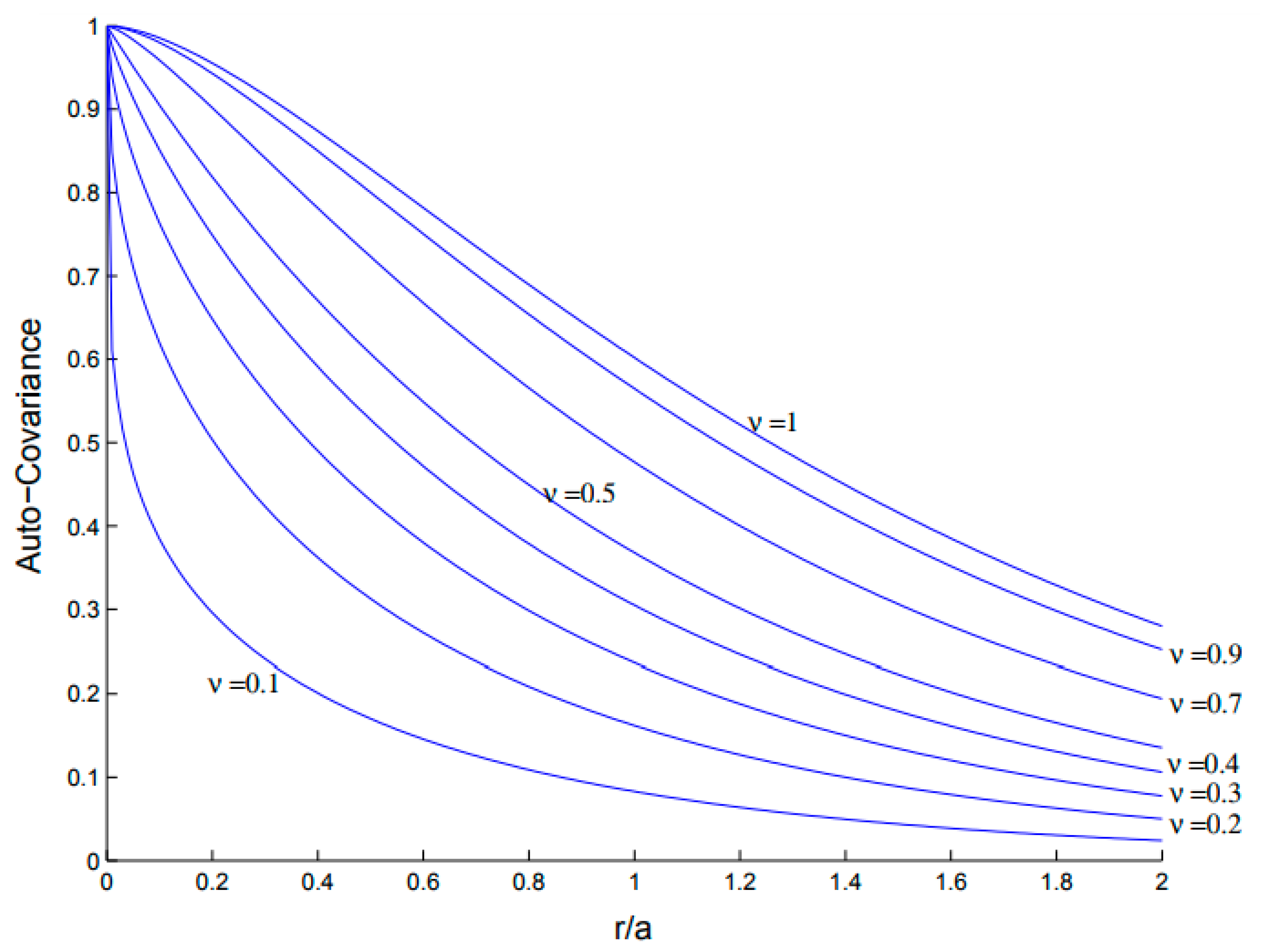
A new version of KIM, named Improved KIM (IKIM), is presented. The proposed IKIM includes the von Karman covariance model whose settings are optimized based on error variance minimization by an evolutionary algorithm.

(2)

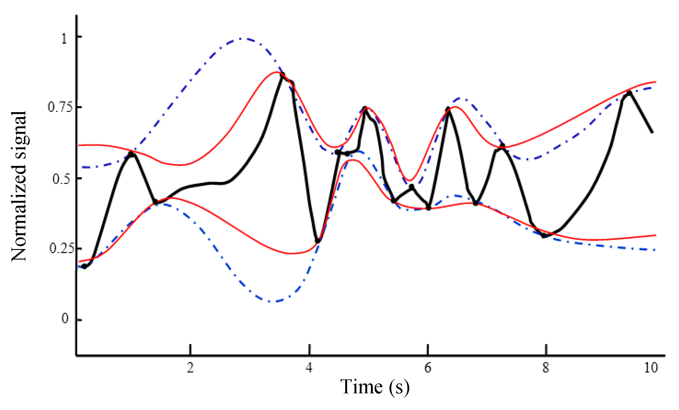
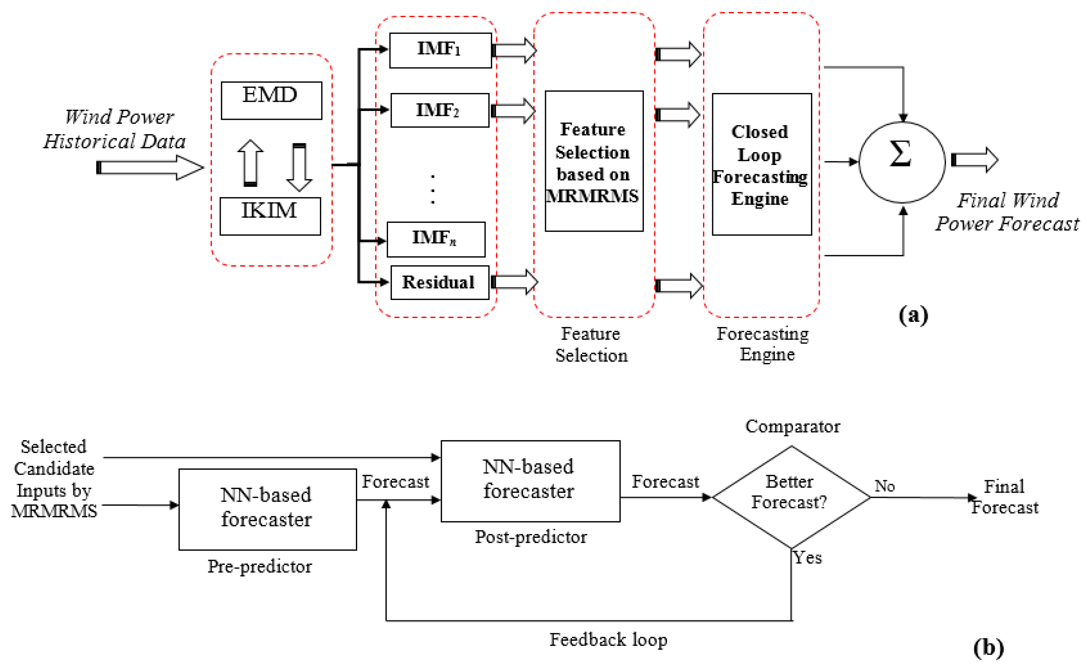
An improved version of EMD is introduced. Cubic spline fitting of conventional EMD is replaced by IKIM in the proposed EMD. It is shown that the proposed EMD alleviates the problems of conventional EMD.

(3)

A new closed-loop forecasting engine is proposed for wind power prediction. This forecasting engine is based on NN trained by Levenberg–Marquardt learning algorithm.

(4)

A new wind power prediction approach is presented, which is composed of the proposed EMD, an information-theoretic feature selection method, and the proposed forecasting engine.

Since stochastic search methods, such as particle swarm optimization (PSO), proceed randomly in the solution space to find the optimal solution, numerical stability is an important concern for these methods. However, we have used Levenberg–Marquardt (LM) learning algorithm, which is an efficient training mechanism for prediction tasks, to train the NN-based forecasting engine. Unlike stochastic search methods, LM does not search randomly the solution space. Instead, LM effectively proceeds in the solution space using Gauss–Newton and steepest descent techniques. Since LM does not have random evolution, numerical stability is not a problem for this method.

Microgrids are small power networks that supply load demands locally. For this purpose, a microgrid provides a system approach to distributed generations. Thus, a microgrid can have both dispatchable units (such as diesel engines and micro-turbines) and renewable units (such as wind units and solar units). If a microgrid has wind units, the proposed wind power prediction approach can be used to forecast its wind power the same as it is used to forecast the wind power of a wind farm. We should give the historical data of the wind power pertaining to the wind units of the microgrid to the proposed prediction approach. The proposed approach decomposes this wind power time series by means of IKIM and EMD, selects most effective features for it by means of Maximum Relevancy, Minimum Redundancy and Maximum Synergy (MRMRMS) feature selection method and provides wind power forecast for the microgrid through the closed-loop forecasting engine. In other words, the proposed wind power prediction approach forecasts wind power of a microgrid based on the same steps and methodology used to forecast wind power of a power system. Thus, the proposed wind power prediction approach can be useful for microgrids the same as it is useful for power systems and wind farms.

The next sections of the paper are structured as follows. In Section 2, conventional EMD is first introduced and then the proposed EMD based on IKIM is presented. In Section 3, the proposed closed-loop forecasting engine and the information-theoretic feature selection method are introduced. Afterwards, the proposed wind power prediction approach is constructed by combining its components. The numerical results produced by the proposed wind power prediction approach for real-world wind farms are presented in Section 4 and compared with the results of many other prediction methods. Section 5 presents a discussion of the results and Section 6 concludes the paper.

2. Empirical Mode Decomposition (EMD)

EMD aims at decomposing a volatile signal to more smooth and well-behaved components called Intrinsic Mode Function (IMF). IMF is an oscillating function, as a counterpart to harmonic function, with two main characteristics: (1) IMF has the same number of local maxima, local minima and zero crossings or at most these numbers differ by one, (2) the mean of IMF is zero. To decompose a signal to IMF components, EMD uses an iterative sifting process that can be summarized as the following step-by-step EMD algorithm:

EMD Algorithm:

(1) Calculate the local maxima and minima of the signal, denoted by x(t), within the considered domain. (2) Connect the maxima of x(t) with an interpolating function, such that an upper envelope u(t) is created about the signal. EMD uses spline of order 3, known as Cubic Spline (CS), for the interpolation [29]. Similarly, connect the minima of x(t) with the interpolating function to create a lower envelope l(t) around the signal. These envelopes are shown in Figure 1. (3) The mean of the upper and lower envelopes, i.e., s(t) = [u(t) + l(t)]/2, is calculated, which is the curve of local mean in Figure 1. (4) If the stopping condition a is satisfied, the local mean s(t) is an IMF and go to step 5; otherwise, substitute the signal with signal minus the local mean, i.e., x(t) − s(t)→x(t), and go back to step 2. (5) Suppose n IMF components s1(t), s2(t), …, sn(t) have been produced so far. Compute the residual r(t) = x(t) − [s1(t) + s2(t) + … + sn(t)]. If the stopping condition b is satisfied, terminate the algorithm; otherwise, substitute the signal with the residual, i.e., r(t)→x(t), and go back to step 2.

The stopping condition a expresses that the relative difference between two successive local means should be less than a threshold [30], which means that iterating the inner loop makes negligible changes in the local mean. The stopping condition b for the outer loop states that the residual should be monotonically increasing or decreasing, i.e., no oscillation is observed in the residual in the considered domain [31]. If the algorithm is terminated with n IMF components, the signal is decomposed as:

$$x(t)={\displaystyle {\sum }_{i=1}^n{s}_i(t)+r(t)}$$

(1)

EMD is an effective signal-processing tool to analyze local behaviors through decomposing a volatile signal into less volatile components. However, it has an important disadvantage, which is generating fake extremes introduced by the CS curve fitting. These fake maxima and minima lead to fake overshoots and undershoots, indicated in Figure 2, which decreases the accuracy of the produced IMFs and also increases the iterations of the sifting process. To cope with these problems and enhance the performance of EMD, a modified version of it is proposed in which the CS interpolation is replaced by IKIM. In the following, ordinary KIM is first reviewed briefly and then an improved version of ordinary KIM, i.e., IKIM, is introduced. Afterwards, the proposed IKIM is applied to EMD.

Kriging is an interpolation method, which estimates the value of a function at a given point as a weighted sum of the function values at the neighboring points [32]. Kriging has important advantages with respect to other interpolation techniques. It assigns weights based on a data-driven strategy, instead of an arbitrary function, giving higher weights to isolated points compared to points within a cluster. Moreover, Kriging can provide an error estimation through Kriging variance along with estimation of the own variable [33].

KIM estimates the value of a time series x(t) at point t, through the following weighted sum:

$$\widehat{x}(t)={\displaystyle {\sum }_{i=1}^M{w}_{i}x(t_i)},{\displaystyle {\sum }_{i=1}^M{w}_i}=1$$

(2)

where $\widehat{x}(t)$ indicates KIM estimation of x(t); t_i, 1 ≤ i ≤ M, are the neighboring points of t.

In ordinary KIM [34], the weights w_i are obtained through variance minimization model. The KIM error, denoted by e(.), for estimation of x(t) is as follows:

$$e[x(t)]=\widehat{x}(t)-x(t)={\displaystyle {\sum }_{i=1}^M{w}_{i}x(t_i)}-x(t)$$

(3)

which can be written in vector form as below:

$$e[x(t)]=\left[w_1\cdots w_M-1\right]{\left[x(t_1)\cdots x(t_M)x(t)\right]}^T$$

(4)

where the superscript T indicates transpose. The error variance, shown by $Var\left(e[x(t)]\right)$, can be written as below based on the bilinear form theorem [35]:

$$\begin{array}{l}Var\left(e[x(t)]\right)=\left[w_1\cdots w_M-1\right].\\ Var\left({\left[x(t_1)\cdots x(t_M)x(t)\right]}^T\right).{\left[w_1\cdots w_M-1\right]}^T\end{array}$$

(5)

By decomposing the vector ${\left[x(t_1)\cdots x(t_M)x(t)\right]}^T$ to two sub-vectors $X={\left[x(t_1)\cdots x(t_M)\right]}^T$ and $[x(t)]$, (5) can be reformulated as:

$$\begin{array}{l}Var\left(e[x(t)]\right)=\left[w_1\cdots w_M-1\right].\\ \left[\begin{array}{l}Var\left(X\right)Cov\left(X,x(t)\right)\\ \left[Cov\left(X,x(t)\right)\right]{}^{T}Var\left(x(t)\right)\end{array}\right].{\left[w_1\cdots w_M-1\right]}^T\end{array}$$

(6)

where Cov(.,.) represents covariance function. Consequently, ordinary KIM determines the weights w₁, …, w_M by solving the following optimization model:

$$\underset{w_1,\dots ,w_M}{{\displaystyle \mathit{M}\mathit{i}\mathit{n}}}\left\{Var\left(e[x(t)]\right)\right\}st.{\displaystyle {\sum }_{i=1}^M{w}_i}=1$$

(7)

where $Var\left(e[x(t)]\right)$ is as presented in (6). To compute the variance and covariance terms of (6), KIM assumes Gaussian process for the M samples (i.e., the prior distribution) and so the resulting posterior distribution becomes Gaussian [33]. The optimization problem of (7) can be solved by means of Lagrange multipliers’ method, which leads to the following solution [34]:

$$\left[\begin{array}{l}{w}_1\\ ⋮\\ w_M\\ \lambda \end{array}\right]={\left[\begin{array}{l}Cov\left(x(t_1),x(t_1)\right)\cdots Cov\left(x(t_1),x(t_M)\right)1\\ ⋮\\ Cov\left(x(t_M),x(t_1)\right)\cdots Cov\left(x(t_M),x(t_M)\right)1\\ 1\cdots 10\end{array}\right]}^{-1}.\left[\begin{array}{l}Cov\left(x(t_1),x(t)\right)\\ ⋮\\ Cov\left(x(t_M),x(t)\right)\\ 1\end{array}\right]$$

(8)

where λ is the Lagrange multiplier associated with the constraint ${\displaystyle {\sum }_{i=1}^M{w}_i}=1$. By determining the weights w₁, …, w_M, the estimation of $x(t)$, i.e., $\widehat{x}(t)$, and the error variance can be obtained through (2) and (6), respectively.

The most time-consuming part of (8) is calculation of the covariance functions. Thus, to decrease the computation burden of the above optimization problem, a well-known approximation for the covariance of Gaussian processes is used here in which the covariance function is approximated based on the covariogram [33]:

$$Cov\left(x(t_i),x(t_j)\right)=C(d_{ij})$$

(9)

where d_ij indicates the Euclidean distance between t_i and t_j. For our one-dimensional problem the Euclidean distance is reduced to d_ij = |t_i − t_j|. Also, C(.) is the covariogram which represents the covariance function based on the distance d_ij. For this purpose, several functions have been presented in the literature as C(.), such as the linear model, the exponential model, the Gaussian model, and the spherical model [34]. Recently, the von Karman covariance model has been introduced in [35], which is an effective model considered for calculating the covariance terms in this work. The anisotropic von Karman function can be defined as:

$$C(r)=\frac{{\sigma }^2}{2^{v-1}\mathsf{\Gamma }(v)}{(r/a)}^v{K}_v(r/a)$$

(10)

where Γ(.) is the gamma function and K_v is the modified Bessel function of the second type of order 0 ≤ v ≤ 1 [36]; r is the lag; a is correlation length; and σ² represents the variance. Figure 3 shows C(r) in terms of r/a for different values of v. In this paper, v = 0.5 is adopted, which leads to exponential auto-covariance function. Moreover, the value of a in C(r) is optimized by Shark Smell Optimization (SSO) method which has been recently introduced in [37]. The objective of this optimization problem is minimizing the error variance. For details of SSO, the interested readers can refer to [37] The proposed IKIM includes KIM with the von Karman covariance model given in (10) and SSO optimization used to optimize the value of a.

The performance of the proposed EMD based on IKIM to decompose a signal x(t) can be summarized as the following steps:

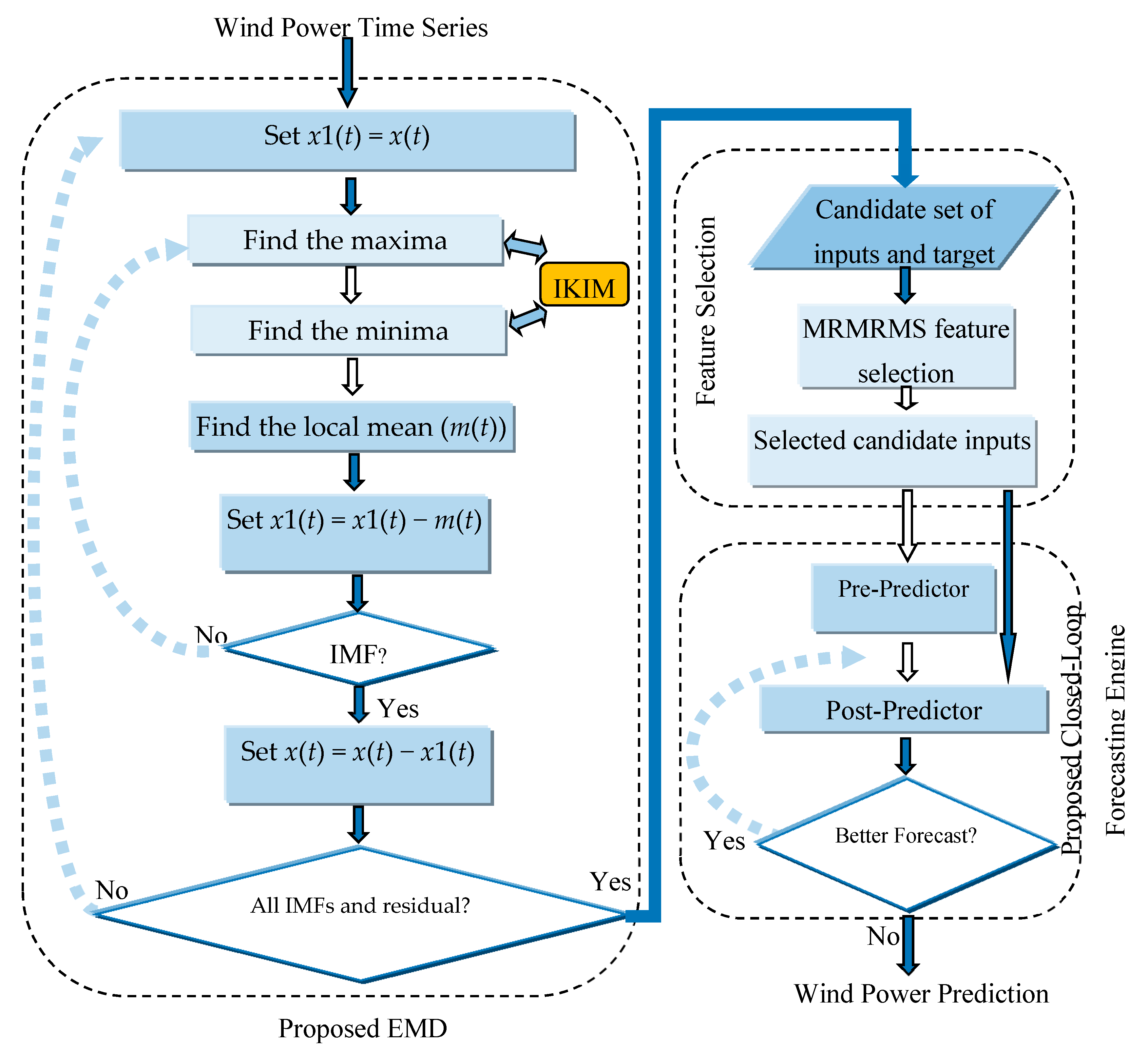
• Set x1(t) = x(t).
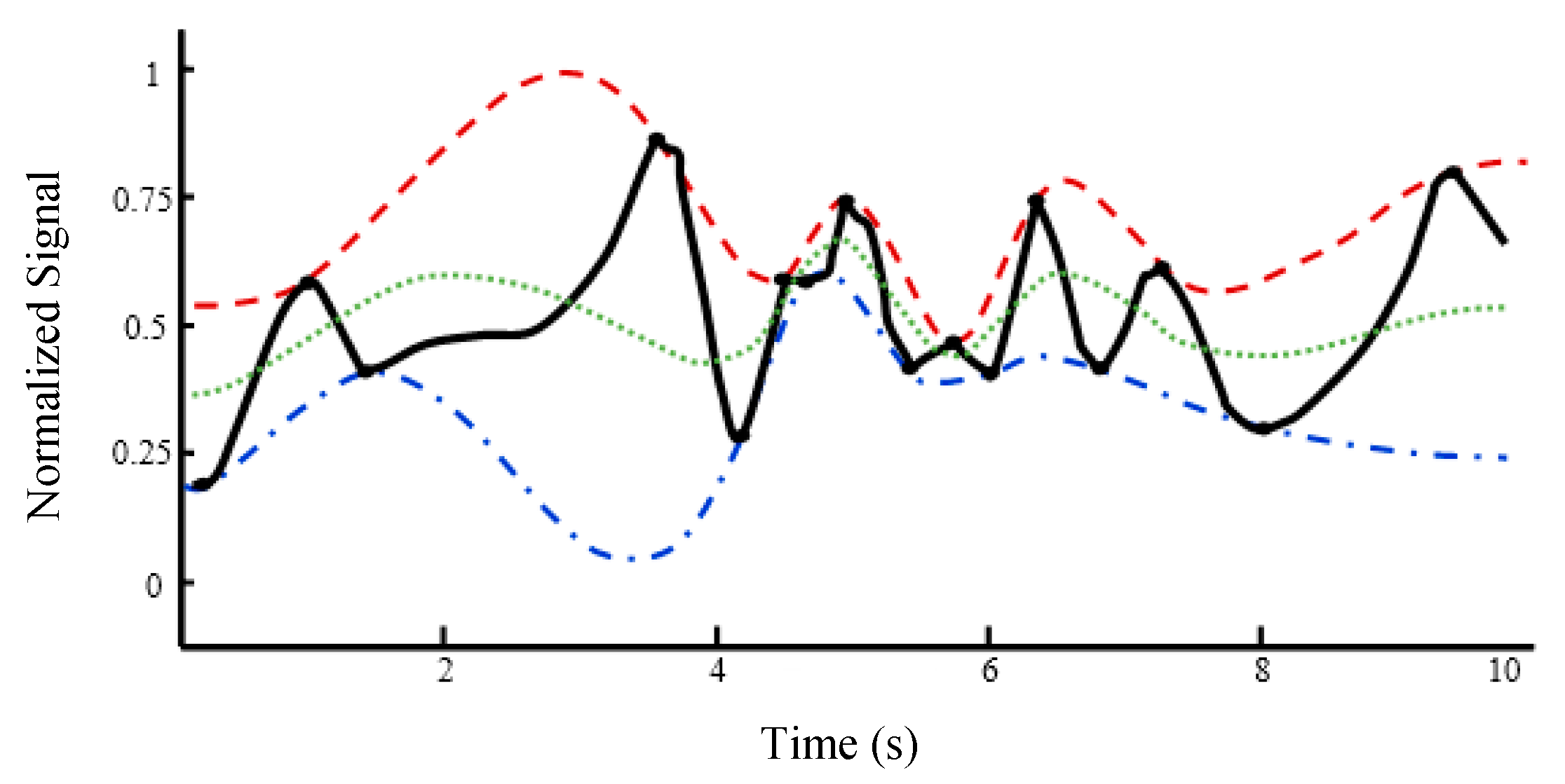
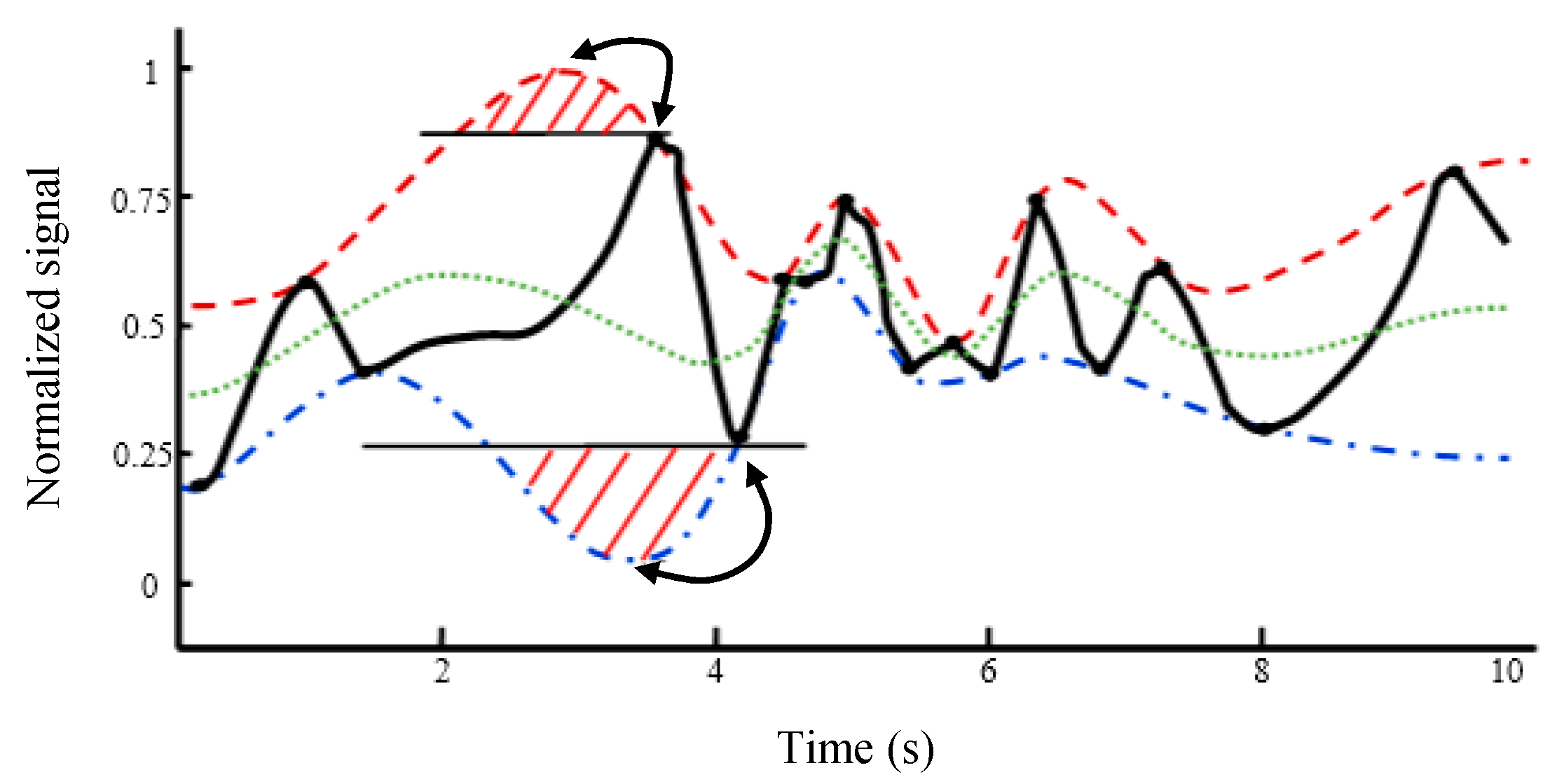
• Find the maxima of the signal x1(t) and obtain the upper envelope ue(t) using the proposed IKIM.
• Find the minima of the signal x1(t) and obtain the lower envelope le(t) using the proposed IKIM.
• Find the local mean m(t) = [ue(t) + le(t)]/2.
• Set x1(t) = x1(t) − m(t) and determine if x1(t) is an IMF or not by checking the properties of IMF. Repeat steps 2 to 5 until x1(t) becomes an IMF. Store the obtained IMF.
• Set x(t) = x(t) − x1(t).
• Repeat steps 1 to 6 until all IMFs and residual of signal x(t) are obtained.

The results obtained from applying the proposed EMD using IKIM to the test case of Figure 2 are shown in Figure 4, which are compared with the results of the conventional EMD using CS. It is seen that the proposed EMD results in more accurate envelopes compared with the conventional EMD. The fake overshoots and fake undershoots of the envelopes generated by the conventional EMD are significantly mitigated in the envelopes generated by the proposed EMD. By generating more accurate envelopes, more accurate IMF components can be produced by the proposed EMD.

3. Proposed Wind Power Prediction Approach

The structure of the wind power prediction approach proposed in this research work is shown in Figure 5a. Within this approach wind power time series is first decomposed using the proposed EMD based on IKIM. Each of IMFs and residual is separately predicted by means of a feature selection method and a closed-loop forecasting engine. The feature selection method receives the historical data of each IMF/residual time series as well as the historical and forecast values of the exogenous variables, e.g., the historical and predicted values of wind speed and temperature provided by Numerical Weather Prediction (NWP). Subsequently, the feature selection method separately selects the candidate inputs that are informative for the forecast process of each IMF/residual. Since wind power is a nonlinear function of the candidate inputs and these candidate inputs can be redundant and interacting, the information-theoretic feature selection method of Maximum Relevancy.

Maximum Relevancy, Minimum Redundancy and Maximum Synergy (MRMRMS) [38] has been used in the proposed wind power prediction approach. The forecasting engine of each IMF/residual is fed by the selected candidate inputs of MRMRMS as shown in Figure 5b. By selecting more relevant, less redundant and more synergetic candidate inputs, the forecasting engine can better extract the input/output mapping function of each IMF/residual. However, since MRMRMS is not a contribution of this article, it is not further discussed here. Details of this method can be found in [38]. Instead, we focus on the forecasting engine in the following, which is one of contributions of this research work.

As seen from Figure 5b, the first block of the proposed closed-loop forecasting engine is a pre-predictor, which is an NN-based forecaster. The output of this pre-predictor and the candidate inputs selected by MRMRMS feature selection method are given to a post-predictor, which is another NN-based forecaster. Both of these NN-based forecasters (i.e., pre-predictor and post-predictor) have Multi-Layer Perceptron (MLP) structure and Levenberg–Marquardt (LM) learning algorithm, which is an efficient training mechanism for the prediction tasks [39]. However, these two forecasters have different roles in the proposed forecasting engine. Pre-predictor forecasts the future values of the associated time series (IMF or residual) using the candidate inputs selected by MRMRMS. This forecast, i.e., the output of pre-predictor, is used as an initial prediction to initialize the feedback loop shown in Figure 5b. Within this feedback loop, the NN-based forecaster of post-predictor predicts the future values of the associated time series using both the selected candidate inputs of MRMRMS and the output of pre-predictor. Since post-predictor has the forecast generated by pre-predictor, which is an input close to the output, it is expected that post-predictor more accurately predicts the future values of the associated time series compared with pre-predictor. The next element in the feedback loop, i.e., comparator, evaluates this aspect. If the forecast of post-predictor is better than the forecast of pre-predictor, the forecast of post-predictor is feed backed through the feedback loop to replace the forecast of pre-predictor at the input of post-predictor. Then, post-predictor forecasts the output using this more accurate input. Similarly, comparator compares the two forecasts at the input and output of post-predictor and if a more accurate forecast is obtained at the output of post-predictor with respect to its input, the process of the feedback loop is repeated.

When no better forecast can be generated by post-predictor or difference between the two forecasts at the input and output of post-predictor becomes negligible, this process is terminated and the last generated forecast by post-predictor is given as the final forecast of the proposed closed-loop forecasting engine.

In practice, since we do not have the output of forecast samples (e.g., hourly wind powers of the next day), validation samples are used instead of forecast samples to evaluate the accuracy of the forecasts generated by pre-predictor and post-predictor. Validation samples are a part of historical data which is not used as training samples and kept unseen for the forecasting engine. Thus, by evaluating the error of validation samples or validation error we can obtain an estimation from forecast error. To attain an accurate estimation of forecast error, validation samples should be as similar as possible to the forecast samples. Thus, in this research work, the hourly samples of the day before the forecast day (which are the closest samples to the forecast samples) are selected as the validation samples.

The flowchart of the whole proposed wind power prediction approach is shown in Figure 6. In this flowchart, the performance of the proposed approach including its various components is illustrated.

4. Numerical Results

The effectiveness of the proposed prediction approach, illustrated in Figure 5a, is extensively evaluated using real-world test cases in this section.

4.1. Sotavento Wind Farm in Spain

Sotavento wind farm is located in Galicia, Spain. It has 24 wind turbines with 17.56 MW nominal power and 38.5 GWh predicted annual production [40]. All data of this test case has been obtained from [40]. The results produced by the proposed prediction approach for this test case are given in

Table 1. Obtained Root Mean Square Error (RMSE) results for day-ahead wind speed forecast of Sotavento wind farm in the four test weeks of year 2005.

Test Week	Correlation Analysis + HIFM [8]	MI-MR Feature Selection + MLP [8]	MI-MR Feature Selection + HIFM [8]	EMD + Cubic Spline	KIM + Gaussian Model	KIM + Exponential Model	KIM + Linear Model	KIM + Spherical Model	Proposed
Feb.	7.56	7.68	5.71	5.08	5.37	2.26	2	1.56	0.98
May	5.82	5.96	4.26	4.14	4.07	3.37	3.07	2.4	1.32
Aug.	6.93	7.01	5.92	4.37	4.08	2.03	1.9	1.28	0.87
Nov.	5.97	6.04	4.55	4.41	4.83	3.35	3.11	2.08	1.34
Ave.	6.57	6.68	5.11	4.5	4.59	2.75	2.52	1.83	1.13

and compared with the results of eight other wind forecast methods. The first three comparative methods of Table 1 are correlation analysis with Hybrid Iterative Forecast Method (HIFM) [8], two stage MI-MR feature selection with MLP forecasting engine [8], and MI-MR feature selection with HIFM [8]. The results presented for these methods in Table 1 have been quoted from [8]. The next five comparative methods of Table 1 consist of classic EMD based on CS as well as KIM based on Gaussian model, KIM based on Exponential model, KIM based on linear model, and KIM based on spherical model which are previous versions of KIM presented in the literature. By comparing with these five methods the effectiveness of the proposed EMD based on IKIM can be evaluated. The same test conditions including the same set of candidate inputs (consisting 200 lagged wind speed hourly values), the same training period (consisting 50 days previous to each forecast day partitioned to 49 days as training period and one day prior to the forecast day as validation set), and the same test periods (consisting the third week of the months February, May, August, and November pertaining to year 2005) have been considered for all forecast methods of Table 1. Since wind speed prediction results in terms of Root Mean Square Error (RMSE) have been presented in [8], this forecast process and error criterion have been considered for all methods of Table 1. RMSE is defined as:

$$RMSE(\mathrm{m}/\mathrm{s})={\left[\frac{1}{N}{\displaystyle \sum _{t=1}^N{\left(X_{ACT(t)}-X_{FOR(t)}\right)}^2}\right]}^{1/2}$$

(11)

where X_ACT(t) and X_FOR(t) indicate actual and forecast values of the time series (here, wind speed time series) for hour t; and N indicates the length of the forecast horizon in terms of hour (here, 24 h for day-ahead forecast). RMSE of each test week, presented in Table 1, is average of its seven daily.

RMSE values are computed using (11). The last row of Table 1 shows average RMSE results of the four test weeks. The RMSE results of Table 1 show that the proposed prediction approach has much lower wind speed forecast errors than all other methods in all test weeks. The comparisons of Table 1 illustrate high forecast accuracy of the proposed approach for wind speed prediction.

4.2. Alberta Test Case

In this test case, we focus on the prediction of the aggregated wind power pertaining to the wind farms of Alberta, Canada [41]. The results produced by the proposed prediction approach for this test case are presented in

Table 2. Obtained results for wind power forecast of the Alberta test case in the four test days of year 2009.

Test Day	Error Criterion	Persistence [25]	BPNN [25]	RBFNN [25]	ANFIS [25]	NN-PSO [25]	WT + BPNN [25]	WT + RBFNN [25]	WT + ANFIS [25]	WT + NNPSO [25]	MI-IG + NN + CSSO [42]	Proposed
3 December	MAPE	10.03	13.62	10.41	14.81	9.54	11.26	8.26	11.08	7.28	7.12	4.18
	NMAE	4.18	4.32	4.61	4.75	4.09	4.29	4.19	4.55	3.87	4.02	3.23
	NRMSE	5.41	5.73	5.84	6.13	5.38	5.44	5.43	5.91	5.07	4.86	3.32
4 May	MAPE	11.31	12.42	11.07	13.51	11.41	11.73	9.22	11.76	8.73	8.50	5.43
	NMAE	4.58	4.88	4.61	4.71	4.51	4.67	4.18	4.39	4.11	4.12	3.12
	NRMSE	6.11	6.38	5.89	6.43	6.20	6.09	5.41	6.22	5.83	5.92	4.13
7 July	MAPE	21.58	17.44	16.72	19.30	12.26	14.11	12.39	16.38	11.27	10.12	7.32
	NMAE	8.48	7.46	7.21	7.75	5.94	6.97	7.04	7.18	5.29	5.10	4.14
	NRMSE	11.25	9.23	8.88	10.16	7.33	8.96	8.36	9.63	7.02	6.76	5.44
15 October	MAPE	14.79	13.93	12.73	12.04	12.82	11.67	14.86	11.08	5.48	5.63	4.07
	NMAE	7.48	7.26	7.31	7.76	6.85	7.14	7.08	7.32	6.17	6.08	5.21
	NRMSE	9.19	8.79	8.99	9.38	7.43	8.22	8.60	8.93	7.21	6.43	5.73
Average	MAPE	14.43	14.35	12.73	14.91	11.51	12.19	11.18	12.57	8.19	7.84	5.25
	NMAE	6.18	5.98	5.93	6.24	5.35	5.77	5.62	5.86	4.86	4.83	3.92
	NRMSE	7.99	7.53	7.4	8.02	6.58	7.18	6.95	7.67	6.28	5.99	4.65

and compared with the results of 10 other methods including persistence method [25], Back Propagation NN (BPNN) [25], Radial Basis Function Neural Network (RBFNN) [25], Adaptive Neuro-Fuzzy Inference System (ANFIS) [25], NN based Particle Swarm Optimization (NNPSO) [25], Wavelet Transform (WT) plus BPNN [25], WT plus RBFNN [25], WT plus ANFIS [25], WT plus NNPSO [25], and Mutual Information with Interaction Gain (MI-IG) feature selection plus NN plus Chaotic SSO (CSSO) [42]. The results of the first nine comparative methods of Table 2 have been quoted from [25] and the results of MI-IG+NN+CSSO have been quoted from [42]. The same test conditions of [25,42] have been also considered for the proposed approach. Based on [25,42], the test period includes four test days of 2009 (which consist of 3 December, 4 May, 7 July, and 15 October) and the error criteria include Mean Absolute Percentage Error (MAPE), Normalized Mean Absolute Error (NMAE), and Normalized RMSE (NRMSE). These error criteria are defined as:

$$MAPE(\%)=\frac{1}{N}{\displaystyle \sum _{t=1}^N\frac{\left|X_{ACT(t)}-X_{FOR(t)}\right|}{{\overline{X}}_{ACT(t)}}}\times 100,{\overline{X}}_{ACT(t)}=\frac{1}{N}{\displaystyle \sum _{t=1}^N{X}_{ACT(t)}}$$

(12)

$$NMAE=\frac{1}{N}{\displaystyle \sum _{t=1}^N\frac{\left|X_{ACT(t)}-X_{FOR(t)}\right|}{X_N}}\times 100$$

(13)

$$NRMSE={\left[\frac{1}{N}{\displaystyle \sum _{t=1}^N{\left(\frac{X_{ACT(t)}-X_{FOR(t)}}{X_N}\right)}^2}\right]}^{1/2}\times 100$$

(14)

where X_ACT(t), X_FOR(t), and N are as defined for (11) except that wind power times series instead of wind speed time series is considered here; and X_N indicates aggregated nameplate capacity pertaining to the wind farms. Table 2 illustrates that the proposed approach has better wind power forecast results than all 10 comparative methods in all four test days and considering all three error criteria. These comparisons clearly illustrate effectiveness of the proposed prediction approach for wind power forecast.

In another numerical experiment performed on the Alberta test case and reported in

Table 3. Obtained results for wind power forecast of the Alberta test case in the four test weeks of year 2012.

Methods	Error Criterion	March Test Week	June Test Week	September Test Week	December Test Week	Ave.
Persistence [43]	NRMSE	13.71	15.14	18.44	12.49	14.95
	NMAE	10.08	10.79	13.11	8.84	10.71
RBF [43]	NRMSE	18.32	14.57	18.62	14.11	16.40
	NMAE	13.32	10.45	13.77	10.24	11.95
MLP [43]	NRMSE	15.36	15.62	19.80	12.32	15.78
	NMAE	12.42	11.56	14.54	9.02	11.89
WNN with MSE [43]	NRMSE	12.38	14.99	17.66	11.65	14.17
	NMAE	9.36	10.64	12.49	8.53	10.26
WNN with MCC [43]	NRMSE	12.23	12.48	16.68	11.58	13.24
	NMAE	9.22	9.64	11.73	8.22	9.70
Proposed	NRMSE	10.10	10.54	14.21	9.32	11.04
	NMAE	7.32	7.47	9.14	6.36	7.57

, the proposed approach is compared with five other methods including persistence method [43], Radial Basis Function (RBF) neural network [43], MLP neural network [39], Wavelet Neural Network (WNN) with Mean Squared Error (MSE) [43], and WNN with Maximum Correntropy Criterion (MCC) [43]. The results of these five comparative methods have been quoted from [43]. The same test conditions of [43] have been considered for the proposed approach in this numerical experiment. Thus, based on [43], 6-h forecast horizon (instead of 24-h forecast horizon adopted for the numerical experiments of Table 1 and Table 2), four test weeks (including the second week of March, June, September, and December of year 2012), and the error criteria NRMSE and NMAE have been considered for the numerical experiment of Table 3. This table shows that the proposed approach has better wind power forecast results than all five comparative methods in all four test weeks and in terms of both NRMSE and NMAE error criteria.

4.3. Blue Canyon Wind Farm

The Blue Canyon wind farm includes 45 turbines with a nameplate capacity of 74 MW [44]. The results obtained from the proposed approach for this test case are presented in

Table 4. Obtained results for wind power forecast of the Blue Canyon wind farm with different forecast horizons.

Test Conditions		Persistence Method [5]	CA+BCD + SVR [5]	MHNN + EPSO [11]	Proposed
Forecast Horizon	Error
1-h. ahead	NMAE	7.84	6.65	4.12	3.87
1-h ahead	NRMSE	11.93	10.54	7.52	5.43
24-h ahead	NMAE	21.24	14.38	7.90	6.64
24-h ahead	NRMSE	29.84	19.74	12.60	10.29
48-h ahead	NMAE	25.42	15.73	10.51	7.89
48-h ahead	NRMSE	34.81	21.24	16.58	14.32

and compared with the results of three other methods including persistence method [5], Correlation Analysis (CA) + Bayesian Clustering by Dynamics (BCD) + Support Vector Regression (SVR) [5], and Modified Hybrid Neural Network (MHNN) + Enhanced Particle Swarm Optimization (EPSO) [11]. The results of the persistence method and CA + BCD + SVR have been quoted from [5] and the results of MHNN + EPSO have been quoted from [11]. The same test conditions of [5,11] have been considered for the proposed approach in this numerical experiment. Accordingly, the test period is the month of June, 2005 in Table 4. Furthermore, three forecasting horizons of 1-h ahead, 24-h ahead, and 48-h ahead are considered in this numerical experiment. From the results of Table 4 it is seen that the proposed method outperforms all three comparative methods in terms of both NMAE and NRMSE error criteria and all three forecast horizons.

Finally, to give graphical insight about the wind power prediction accuracy of the proposed approach, the forecast, actual, and forecast error curves for a sample day 25 June 2005 are shown in Figure 7. This figure shows that while wind power actual curve has irregular patterns and sudden changes, the forecast curve generated by the proposed approach reasonably follows the actual curve and the forecast error curve has small values, which indicate good performance of the proposed approach.

5. Discussion

In this research work, the effectiveness of the proposed prediction approach has been extensively illustrated through four numerical experiments for both wind speed and wind power forecast on three real-world test cases. In these four numerical experiments, the proposed prediction approach has been compared with many other forecast methods in terms of various error criteria and with different forecast horizons. In the first, second, third, and fourth numerical experiment, the proposed method has been compared with eight other methods, 10 other methods, five other methods, and three other methods, respectively. Thus, the paper presents a total of 26 numerical comparisons between the proposed approach and other wind power forecast methods. Among these 26 numerical comparisons, 21 comparative results have been taken from previous works. It has been shown that the proposed method outperforms all other methods in these 26 numerical comparisons. Moreover, significant differences are seen between the results of the proposed method and other comparative methods. For instance, in terms of average results obtained in the second numerical experiment (which have been presented in the last row of Table 2), the proposed approach has (7.84 − 5.25)/7.84 × 100% = 33.0% lower MAPE, (4.83 − 3.92)/4.83 × 100% = 18.8% lower NMAE, and (5.99 − 4.65)/5.99 × 100% = 22.4% lower NRMSE than MI-IG+NN+CSSO which is the most accurate comparative method in this numerical experiment. To the best of our knowledge, other published wind power forecast works have less numerical comparisons than our paper.

In addition to tabular results, a graphical illustration of the performance of the proposed approach has been presented. It has been shown that wind power time series has irregular patterns as well as sudden changes and ramps. However, unlike these complex behaviors of wind power time series, the forecast curve generated by the proposed approach reasonably follows the actual curve and the forecast error curve has small values, which indicate good performance of the proposed wind power forecast method.

6. Conclusions

This paper presents a new wind power prediction approach. Higher effectiveness of the proposed approach compared with 26 other wind power forecast methods has been extensively illustrated in the paper. By providing more accurate wind power forecasts than previous methods, the proposed wind power prediction approach can be useful for both wind farm owners and power system operators. With more accurate wind power forecasts, wind farm owners can gain more profits in electricity markets and power system operators need less reserves to cope with the uncertain nature of wind power which in turn decreases the operation cost of wind power-integrated power systems. In addition to wind farms and power systems, the proposed wind power prediction approach can be also useful for microgrids. With more accurate wind power prediction results, a microgrid operator can better manage its wind units and transactions with the upstream grid to decrease its operations costs and obtain more benefits.

Within the proposed approach, wind power time series is first decomposed through a new EMD based on IKIM. In this way, a complex wind power time series is decomposed to its various frequency components, which can be analyzed and predicted more effectively. Afterwards, an information-theoretic feature selection method selects the most effective candidate inputs to predict each component. A closed-loop forecasting engine learns the input/output relation between these selected candidate inputs and the output, i.e., the future value of the associated time series. Unlike conventional open-loop forecast methods, the proposed closed-loop forecasting engine uses an effective feedback of the output to enhance the efficiency of the training process.

While the proposed prediction approach has high forecast accuracy, it can provide point forecast for wind power. Extending the proposed approach to probabilistic forecast, i.e., predicting wind power density function, can be considered as the future work. Predicting wind power density function can be used, for instance, to generate scenarios which are required in stochastic programming methods.

References

- Manzano-Agugliaro, F.; Alcayde, A.; Montoya, F.G.; Zapata-Sierra, A.; Gil, C. Scientific production of renewable energies worldwide: An overview. Renew. Sustain. Energy Rev. 2013, 18, 134–143. [Google Scholar] [CrossRef]
- Hernández-Escobedo, Q.; Manzano-Agugliaro, F.; Zapata-Sierra, A. The wind power of Mexico. Renew. Sustain. Energy Rev. 2010, 14, 2830–2840. [Google Scholar] [CrossRef]
- Hernández-Escobedo, Q.; Manzano-Agugliaro, F.; Gazquez-Parra, J.A.; Zapata-Sierra, A. Is the wind a periodical phenomenon? The case of mexico. Renew. Sustain Energy Rev. 2011, 15, 721–728. [Google Scholar] [CrossRef]
- Montoya, F.G.; Manzano-Agugliaro, F.; López-Márquez, S.; Hernández-Escobedo, Q.; Gil, C. Wind turbine selection for wind farm layout using multi-objective evolutionary algorithms. Expert Syst. Appl. 2014, 41, 6585–6595. [Google Scholar] [CrossRef]
- Fan, S.; Liao, J.R.; Yokoyama, R.; Chen, L.; Lee, W.J. Forecasting the Wind Generation Using a Two-Stage Network Based on Meteorological Information. IEEE Trans. Energy Convers. 2009, 24, 474–482. [Google Scholar] [CrossRef]
- Khosravi, A.; Nahavandi, S.; Creighton, D. Prediction intervals for short-term wind farm power generation forecasts. IEEE Trans. Sustain. Energy 2013, 4, 602–610. [Google Scholar] [CrossRef]
- Jónsson, T.; Pinson, P.; Nielsen, H.A.; Madsen, H.K.; Nielsen, T.S. Forecasting Electricity Spot Prices Accounting for Wind Power Predictions. IEEE Trans. Sustain. Energy 2013, 4, 210–218. [Google Scholar] [CrossRef]
- Amjady, N.; Keynia, F.; Zareipour, H. A New Hybrid Iterative Method for Short Term Wind Speed Forecasting. Eur. Trans. Electr. Power 2011, 21, 581–595. [Google Scholar] [CrossRef]
- Amjady, N.; Keynia, F.; Zareipour, H. Short-term wind power forecasting using ridgelet neural network. Electr. Power Syst. Res. 2011, 81, 2099–2107. [Google Scholar] [CrossRef]
- Chang, W.Y. Short-Term Wind Power Forecasting Using the Enhanced Particle Swarm Optimization Based Hybrid Method. Energies 2013, 6, 4879–4896. [Google Scholar] [CrossRef]
- Amjady, N.; Keynia, F.; Zareipour, H. Wind Power Prediction by a New Forecast Engine Composed of Modified Hybrid Neural Network and Enhanced Particle Swarm Optimization. IEEE Trans. Sustain. Energy 2011, 2, 265–276. [Google Scholar] [CrossRef]
- Soman, S.S.; Zareipour, H.; Malik, O.; Mandal, P. A review of wind power and wind speed forecasting methods with different time horizons. In Proceedings of the North American Power Symposium (NAPS), Arlington, TX, USA, 26–28 September 2010; pp. 1–8. [Google Scholar]
- Wang, X.; Guo, P.; Huang, X. A Review of Wind Power Forecasting Models. Energy Procedia 2011, 12, 770–778. [Google Scholar] [CrossRef]
- Lei, M.; Shiyan, L.; Chuanwen, J.; Hongling, L.; Yan, Z. A review on the forecasting of wind speed and generated power. Renew. Sustain. Energy Rev. 2009, 13, 915–920. [Google Scholar] [CrossRef]
- Chang, W.Y. A Literature Review of Wind Forecasting Methods. J. Power Energy Eng. 2014, 2, 161–168. [Google Scholar] [CrossRef]
- Hassan, S.Z.; Li, H.; Kamal, T.; Arifoglu, U.; Mumtaz, S.; Khan, L. Neuro-Fuzzy Wavelet Based Adaptive MPPT Algorithm for Photovoltaic Systems. Energies 2017, 10, 394. [Google Scholar] [CrossRef]
- Ou, T.C.; Hong, C.M. Dynamic operation and control of microgrid hybrid power systems. Energy 2014, 66, 314–323. [Google Scholar] [CrossRef]
- Hong, C.M.; Ou, T.C.; Lu, K.H. Development of intelligent MPPT (maximum power point tracking) control for a grid-connected hybrid power generation system. Energy 2016, 50, 270–279. [Google Scholar] [CrossRef]
- Shiau, J.K.; Wei, Y.C.; Lee, M.Y. Fuzzy Controller for a Voltage-Regulated Solar-Powered MPPT System for Hybrid Power System Applications. Energies 2015, 8, 3292–3312. [Google Scholar] [CrossRef]
- Fumi, A.; Pepe, A.; Scarabotti, L.; Schiraldi, M.M. Fourier Analysis for Demand Forecasting in a Fashion Company. Int. J. Eng. Bus. Manag. 2013, 30, 10. [Google Scholar] [CrossRef]
- Amjady, N.; Keynia, F. Day ahead price forecasting of electricity markets by a mixed data model and hybrid forecast method. Int. J. Electr. Power Energy Syst. 2008, 30, 533–546. [Google Scholar] [CrossRef]
- Mishra, S.; Sharma, A.; Panda, G. Wind Power Forecasting Model using Complex Wavelet Theory. In Proceedings of the 2011 International Conference on Energy, Automation, and Signal (ICEAS), Bhubaneswar, India, 28–30 December 2011; pp. 1–4. [Google Scholar]
- Catalão, J.P.S.; Pousinho, H.M.I.; Mendes, V.M.F. Hybrid wavelet-PSO-NFIS approach for short-term wind power forecasting in Portugal. IEEE Trans. Sustain. Energy 2011, 2, 50–59. [Google Scholar]
- Wang, J. A Hybrid Wavelet Transform Based Short-Term Wind Speed Forecasting Approach. Sci. World J. 2014, 2014, 1–12. [Google Scholar] [CrossRef] [PubMed]
- Mandal, P.; Zareipour, H.; Rosehart, W.D. Forecasting aggregated wind power production of multiple wind farms using hybrid wavelet-PSO-NNs. Int. J. Energy Res. 2014, 38, 1654–1666. [Google Scholar] [CrossRef]
- Huang, N.E.; Shen, Z.; Long, S.R.; Wu, M.C.; Shih, H.H.; Zheng, Q.; Yen, N.C.; Tung, C.C.; Liu, H.H. The empirical mode decomposition and the Hilbert spectrum for nonlinear and non-stationary time series analysis. Proc. R. Soc. Lond. A 1998, 454, 903–995. [Google Scholar] [CrossRef]
- Wang, D.; Yue, C.; Wei, S.; Lv, J. Performance Analysis of Four Decomposition-Ensemble Models for One-Day-Ahead Agricultural Commodity Futures Price Forecasting. Algorithms 2017, 10, 108. [Google Scholar] [CrossRef]
- Hong, Y.Y.; Yu, T.H.; Liu, C.Y. Hour-Ahead Wind Speed and Power Forecasting Using Empirical Mode Decomposition. Energies 2013, 6, 6137–6152. [Google Scholar] [CrossRef]
- Pegram, G.G.S.; Peel, M.C.; Mcmahon, T.A. Empirical mode decomposition using rational splines: An application to rainfall time series. Proc. R. Soc. A 2008, 464, 1483–1501. [Google Scholar] [CrossRef]
- Barnhart, B.L. The Hilbert-Huang Transform: Theory, Applications, Development. Ph.D. Thesis, The University of Iowa, Iowa City, IN, USA, 2011. [Google Scholar]
- Bohling, G. KRIGING. Available online: http://people.ku.edu/~gbohling/cpe940/Kriging.pdf (accessed on 9 November 2017).
- Li, J.; Heap, A.D. A Review of Spatial Interpolation Methods for Environmental Scientists; Geoscience Australia Record; Geoscience Australia: Canberra, Australia, 2008.
- Huang, Z.; Wang, H.; Zhang, R. An Improved Kriging Interpolation Technique Based on SVM and Its Recovery Experiment in Oceanic Missing Data. Am. J. Comput. Math. 2012, 2, 56–60. [Google Scholar] [CrossRef]
- Williams, C.K.I. Prediction with Gaussian Processes: From Linear Regression to Linear Prediction and Beyond. Available online: https://pdfs.semanticscholar.org/dcd0/a9b1921a34c37f082d03a4d240c9085351c7.pdf (accessed on 9 November 2017).
- Sidler, R.; Holliger, K. Kriging of Scale-Invariant Data: Optimal Parameterization of the Autocovariance Model. In Proceedings of the American Geophysical Union Spring Meeting, San Francisco, CA, USA, 13 December 2004. [Google Scholar]
- Goff, J.A.; Jennings, J.W. Improvement of Fourier-based unconditional and conditional simulations for band-limited fractal (von Kármán) statistical models. Math. Geol. 1999, 31, 627–649. [Google Scholar] [CrossRef]
- Abedinia, O.; Amjady, N.; Ghasemi, A. A New Meta-heuristic Algorithm Based on Shark Smell Optimization. Complexity 2016, 21, 97–116. [Google Scholar] [CrossRef]
- Abedinia, O.; Amjady, N.; Zareipour, H. A New Feature Selection Technique for Load and Price Forecast of Electrical Power Systems. IEEE Trans. Power Syst. 2017, 32, 62–74. [Google Scholar] [CrossRef]
- Amjady, N.; Keynia, F. Day-Ahead Price Forecasting of Electricity Markets by Mutual Information Technique and Cascaded Neuro-Evolutionary Algorithm. IEEE Trans. Power Syst. 2009, 24, 306–318. [Google Scholar] [CrossRef]
- Sotavento Wind Farm. Available online: www.sotaventogalicia.com (accessed on 26 June 2015).
- Alberta Wind Farms. Available online: http://canwea.ca/wind-energy/alberta/ (accessed on 28 June 2015).
- Abedinia, O.; Amjady, N. Short-Term Wind Power Prediction based on Hybrid Neural Network and Chaotic Shark Smell Optimization. Int. J. Precis. Eng. Manuf. Green Technol. 2015, 2, 245–254. [Google Scholar] [CrossRef]
- Chitsaz, H.; Amjady, N.; Zareipour, H. Wind power forecast using wavelet neural network trained by improved Clonal selection algorithm. Energy Convers. Manag. 2015, 89, 588–598. [Google Scholar] [CrossRef]
- Oklahoma Wind Farm. Available online: http://bluecanyonwindfarm.com (accessed on 5 July 2015).