The OBE is the result of indicators used to include the calculation of availability, performance and quality in the respective of bike trips. The aim of this new metric is to identify the losses on BSS and establish a complete understanding of the BSS in terms of availability, performance and quality. The identification and measurement of these efficiencies allow the operator to implement the necessary corrective actions to improve the service.
3.1. Formal Definition and Running Example
Most of the BSS will record data of the bike ID, start time of the trip, end time of the trip, duration of the trip (in second), origin station, destination station and some other external attributes such as riders profile, station ID, zip code, etc.. This study uses only the relevant attributes to enhance the effectiveness measure.
Table 1 shows the fragment of bike trip data used in this study. Note that the time granularity used by most BSS is at the level of minutes while the duration is recorded in seconds. Formal definitions are required to express the time aspects on BSS.
Let E be a set of trip of bikes. A trip log (L) is a collection of trips represented as a tuple of the form bike ID, start trip (ST), end trip (ET), duration (D), origin station (SS), destination station (ES) and rider’s type (U). Note that the riders’ type consists of customer and subscriber. The former refers to the general rider while the latter denotes riders who subscribe as the BSS members. A sequence of trip is denoted as σ = <e1, e2, ..., en> E* where each ei denotes the i-th trip of a bike and n ∈ denotes as the total trip within a period of time.
Suppose that S is a set of stations, thus SS ⋃ ES is a subset of S. The notation e.id, e.st, e.et, e.d, e.ss, e.es, e.u are used to represent bike ID, start trip time, end trip time, trip duration, origin station, destination station and rider’s type, respectively. For example, e = (“1”, “2015-02-24 11:24:00”, “2015-02-24 11:31:00”, 425, A, B, “Subscriber”), then e.id = “1”, e.st = “2015-02-24 11:24:00”, e.et = “2015-02-24 11:31:00”, e.d = 425, e.ss = “A”, e.es = “B”, and e.u = “Subscriber”.
To indicate the bike, the notation
k = 1, …,
K is used to represent the
k-th bike. Hence, a sequence for the trip of bike
k is denoted as
σk = <
ek1,
ek2, ...,
ekn> ∈
E* where
eki ∈
E is a single trip for 1 <
i <
Ik and
Ik is the total trip of the
k-th bike. Referring to
Table 1, bike ID #1 (
k = 1) has five trips (called the actual trip frequency) and it can be denoted as
I1 = 5.
As illustrated in a frequency-based measure by many BSS, it takes into account the actual trip frequency. The total trip frequency of all bikes is commonly used as a measure to indicate the popularity of the BSS. Rather using the total trip frequency, this study uses ratio to represent the BSS performance. Rate (
Rk) is the ratio of actual trip frequency (
Ik) with the best trip frequency, referred to the maximum of actual trip frequency among the active bikes
K (Equation (2)).
3.2. Definition of Overall Bike Effectiveness (OBE)
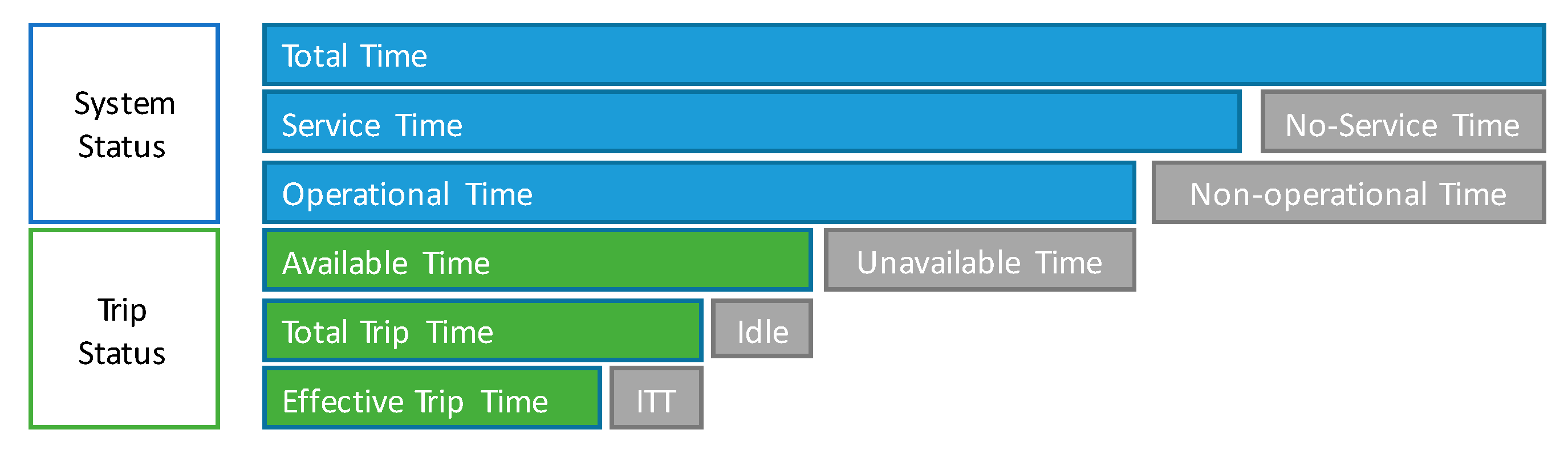
OBE is a term with some metrics to evaluate the effectiveness of BSS. There are six basic time statuses, including total time, service time, operational time, available time, total trip time and effective trip time. Each of the statuses corresponds to an operational state of a particular BSS and a bike. Thus, OBE indices can be defined with system status and trip status. In detail, the OBE framework with regard to time is illustrated in
Figure 2.
System status refers to operational information from the BSS. Meanwhile, trip status is derived from the trip data provided by a particular BSS. Generally, there are three system statuses in BSS; total time, service time and operational time. These statuses focus on the BSS operational aspects as a resolution for improving bike effectiveness. The other three statuses, i.e., available time, total trip time and effective trip time refer to the trip or operational views. These statuses would be used as the basis for assessing the performance measure using OBE.
Total time refers to a particular time period for performance measures. A selected time period, i.e., a week, a month, a year, can be a reference for the basis of the analysis. The total time can be divided into two, i.e., no-service time and service time, to identify and analyze hidden performance loss. Service time refers to the time when the BSS operates. The loss in this time is labeled as no-service time which refers to the time limitation of the system due to public policy in each respective city. For example, BSS in Rio de Janeiro opens the service from 6.00 a.m. to 10.00 p.m. Therefore, the no service time equals 8 h/day. In the case of weekly basis analysis, the service time of the framework would be ((24 h − 8 h) × 7 days) = 112 h. In a different aspect, service time can also be considered as a virtual period when a user requires reserving a bike to ride on. For example, Grid bikes will allow the user to reserve a bike at a particular time [
45]. In this study, the service time refers to the real-world time.
Operational time (O) can be defined as the time on which a bike can be used. Some scheduled maintenance can be one of the reasons on service time reduction which refers to the losses labeled as non-operational time. Although maintenance issues take important roles on the performance measures, it is difficult to specify the exact execution time. If such information is not available, the service time could be directly regarded as operational time.
Available Time denotes the time of a bike liveliness (i.e., in an available state) during the operational time. In other words, the available state refers to the time when a bike keeps performing on the system and is ready to be used. In contrast, the unavailable state is the time when the bike is unavailable from a particular time point in the respective of time analysis unit. These states, available and unavailable, are purposely for measuring the bike availability. Hence, the available time of
k-th bike (
ATk) can be derived by subtracting the end time of the last event with the start time of the first event of a particular bike. Bike Availability of
k-th bike (
Ak) is the proportion of bike available time in regards to the operational time. To measure the bike availability of the system, average bike availability is used. Average Bike Availability (
) can be derived by summing all
k-th bike available time and dividing it with the available bikes (
K) in the period. Note that the available bikes in the period could be different with the available bikes in other period due to the non-operational time such as maintenance. Equations (3)–(5) show the formula to measure bike available time, bike availability and average bike availability, respectively.
Average Bike Availability () can be regarded as a measure to ensure the availability of bikes in the system during the operational time. The can be used to understand any situations which cause low availability. For example, severe damages of bikes without any further action from the operator could cause an unavailable state in the stations.
Table 1 shows there are seven available bikes during three days of operational time. The available time of bike #1 (
AT1) was derived by subtracting the end trip of the last event (“2015-02-26 22:51:00”) with the start trip of the first event (“2015-02-24 11:24:00”). Hence, the
AT1 is 3567 min. The
A1 (the availability of bike #1) would be a division of
AT1 with the operational time (3567/4320 = 0.8256). Finally, the bike availability of the respective BSS (
) is measured by dividing the summation of all bike availability with the number of available bikes. Thus, the bike availability is 49.49% (refer to
Table 2).
Trip time is the duration of a bike used by a rider. In some BSSs, the trip time has been stored in the time unit of ‘second’ as a trip duration although the trip data includes the starting and the ending time of one bike along with riders and stations data. Hence, the total trip time of the k-th bike (TTTk) is the summation of the trip time of k-th bike in the period. To measure the bike performance, it is necessary to know the maximum (best) trip time (TTTbest) in the system in a particular period.
There are two ways to determine the best total trip time (
) based on the period
p. First, the value can be determined by selecting
p as the best period in the previous year. For example, if the current period of analysis is March 2014, then the period
p refers to the month in the previous year which returns the best value. Second, the
p could refer to the same period of the previous year, or year-over-year basis. For example, if the current period is March 2014, then the period
p refers to March 2013. The first approach has less accuracy than the second approach due to seasonal aspects, i.e., weather differences, particular events, etc., with the respective period. In addition, the selection of
p can be different among BSS in accordance to the factors that the operators want to analyze. Hence, the performance of the
k-th bike (
Pk) is the fraction of total trip time (
TTTk) and the best total trip time in the system (
TTTbest). Average Bike Performance (
) can be derived by summing all
k-th bike performance and dividing it with the available bikes (
K) in the period. The Equations (6)–(9) show the total trip time, the best total trip time, bike performance and average bike performance, respectively.
In many cases, the BSS records the duration of a trip. Since some of the BSS stored a coarse-grained time data (i.e., the smallest time unit is stated as ‘minute’), the duration would be more representative to express the fine-grained time data. For example, the first trip of bike #1 has a duration of 425 s meanwhile the difference between the start trip and the end trip result 420 s. By summing all the duration of the bike #1, the total trip (TTT1) is 1,996 s during 3 days operational time. The maximum of trip time among all bikes are the bike #6 which reach 14,580 s, assuming that there is no previous year data. Hence, the bike performance (P6) of bike #6 is 100% and other bikes’ performance follows each of the trip time. Finally, the average of bike performance is evaluated by dividing the summation of all bike performance with the number of available bikes in the period.
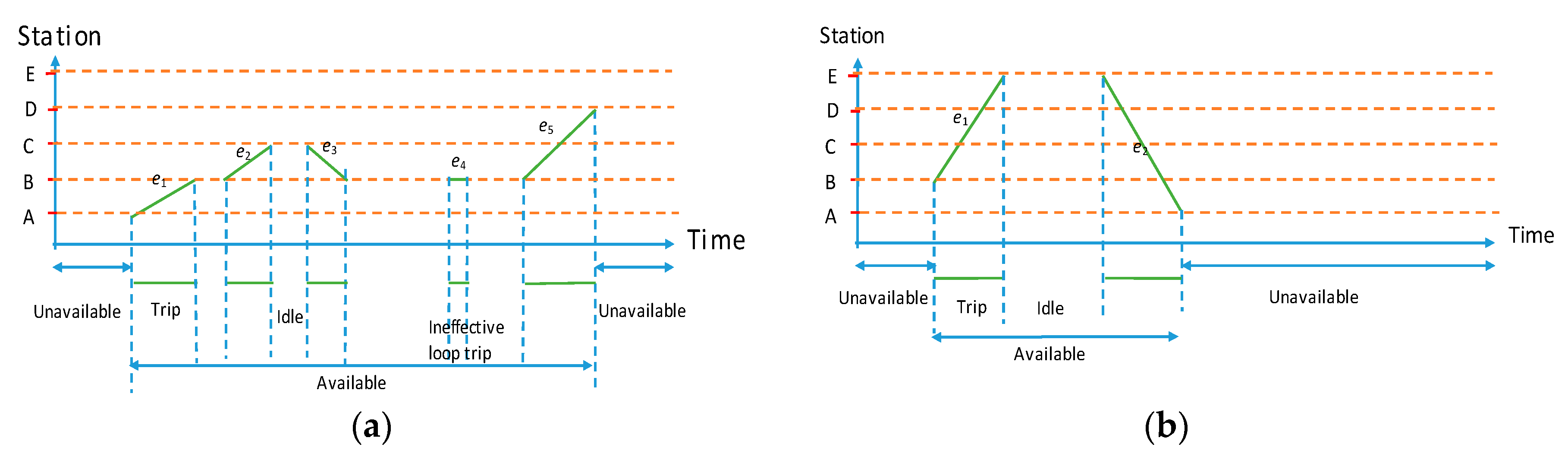
Effective Trip Time is the trip time when a bike is properly used during the trip. To measure the effective trip time, it is necessary to understand the ineffective trip time. There are two types of the ineffective trip; ineffective loop trip time and low utility trip. The ineffective loop time of the
k-th bike (
ILTk) denotes a trip which (1) the destination is the same as the origin (loop trip) and (2) short trip time. For example, a rider may discharge a bike from a station and return it to the original station due to some problems, e.g., flat tires, which rise the rider’s unsatisfactory. The low utility trip of the
k-th bike (
LUTk) refers to a trip which the
TTTk in the analysis period including the frequency of bike usage is less than the standard set by the operator. There are two types of low utility trip; low utility total trip time and low utility trip frequency. For example, the operator sets a bike should be used at least 5 times and more than 60 min of total trip time in a day. Otherwise, the bike is considered as having an ineffective trip time due to the low utility trip. Hence, the effective trip time of
k-th bike (
ETTk) can be derived by subtracting the total trip time (
TTTk) with the ineffective trip time (
ITTk). Note that the ineffective trip time is the summation of the ineffective loop trip and low utility trip. The notion of quality of the
k-th bike (
Qk) means the fraction of effective trip time from the total trip time of the bike. Average Bike Quality (
) can be derived by summing all
k-th bike quality and dividing it with the available bikes (
K) in the period. The Equations (10)–(15) describe the ineffective loop trip, low utility trip, ineffective trip time, effective trip time, bike quality and average bike quality, respectively.
The notation
,
and
refer to the threshold for ineffective loop trip, low utility total trip time and low utility trip frequency, respectively. Note that those thresholds would be determined by the BSS operators and varied according the implemented BSS. BSS which applies free-of-charge pricing structure on the earliest hour of rental would have different threshold with other BSS. For example, Barcelona BSS and most United States (US)-based BSS consider the first 30 min of rental as free-of-charge [
15]. However, YouBike (Taipei) charges the riders from the first time the bike discharges from the station [
46]. Hence, the ineffective loop trip time would be varied according to the policy of the local BSS. For the low utility trip, the thresholds would be based on the target of the BSS operators. For early stage of BSS, operators could not set a high standard. When the BSS becomes stable, operators can increase the threshold to improve the BSS. As a result, the OBE of the
k-th bike is referred to the product of bike availability, bike performance and bike quality expressed as Equation (16). To obtain the overall performance of the BSS, the average of OBE is derived as denoted in Equation (17).
The fragment data in
Table 1 would be used to illustrate the calculation of OBE. A visualization for explaining each of the terminology mentioned in
Figure 2 can be seen in
Figure 3. The calculation begins by determining the operational time and subsequently measures the performance within three statuses; available time, trip time and effective trip time. The total time would be determined by the analyst.
Table 1 illustrates a BSS with a total time of 3 days (4320 min or 259,200 s). Assuming that the BSS operates in 24 h, the service time is considered the same as the total time of 3 days. Since no particular information about maintenance and other issues on operating hours during the period of the fragment trip data, the operational time is considered being equal to the service time.
Measuring bike quality begins by identifying the low utility trip and ineffective loop trip. In many cases, this identification is a challenging assessment since it is hidden in the bike trip. Note that this calculation example is based on a small dataset from
Table 1. The threshold could be set either manually by operators or statistically measured from the data. For example, the low utility trip frequency is lower than or equal to the average of the frequency of all bikes (e.g., 3.4) and the low utility total trip time of each bike is lower than a value, e.g., a standard set by the operator. Assuming that a daily trip time should be greater than 300 s. Since the operational time of the dataset is 3 days, the threshold will count 900 s. Hence, the bike ID #4, #5 and #7 are in the category of since the total trip time of the three bikes is less than 900 s. The ineffective loop trip is measured by pointing a trip that has the same origin and destination and is less than 119 s. Note that the basis of this measure varies according to the policy of BSS. Based on
Table 1, bike ID #1 has 1 occurrence of ineffective loop trip with a duration of 118 s. The effective trip time is derived by subtracting the total trip time with low utility trip and ineffective loop trip. The quality of bike #1 is assessed as (1996 − 118)/1996 = 0.9408. Using the same ways as other bikes, the
is 56.29 which is obtained as the average of
Qk from all bikes.
The overall bike effectiveness of each bike is the multiplication of the three factors. For example, the OBE of bike #1 is 82.56% × 13.68% × 94.08% = 10.62%. Hence, the OBE, as the overall bike effectiveness of the BSS, is the average of the OBE of all bikes, 8.94%. Note that it is rare to get 0% of the
k-th bike OBE in the real world data. However, the existence of 0% of OBE would be very important analysis for the operator to improve the BSS. The detail time derivation for effectiveness calculations is illustrated in
Table 2.
3.3. Directions for Enhancement—Theoretical-Based OBE
The proposed OBE frameworks and indices basically align with a stable BSS. As aforementioned, the newly established BSS is limited on determining some parameters, i.e., the best total trip time (TTTbest) within a period of time. In addition, the bike available time on the new BSS would be less than the stable BSS. As a result, the OBE result would be very low and probably mislead toward termination action. Hence, alternative measures to represent the performance of early generated BSS is necessary. This section addresses the directions for enhancement of actual-based OBE toward theoretical-based OBE (TOBE).
Some newly established BSSs would have many issues on the availability since it requires weeks or even months for introducing the benefit to the society. In the early stage of the BSS, there would be fewer riders which will indirectly reduce the available time and increase operational cost. As a consequence, theoretical-based measurement is likely useful to assess the effectiveness of BSS. However, determining the bike available time would be an issue of measuring the bike availability. Rather than using the actual-based measure, the early stage of BSS could apply the theoretical-based measure. In this case, the theoretical bike availability (
TA) is obtained by calculating the proportion of a number of available bikes (
K) in the period with the number of installed bike provided by the operators (
κ).
Note that the number of installed bikes refers to the number of fleets provided by the operators in the respective BSS. The number of available bikes could be assessed by extracting the bike used by riders within a period of time. If the number of available bikes the same as the number of installed bikes, then the TA is 100%. The loss would be caused by maintenance or replacement issues in a particular period.
The early stage of BSS is also likely to have performance stability issues in comparison to the stable BSS. Measuring the best total trip time is less considered due to instability. Instead, theoretical bike performance (
TP) can be assessed based on the target trip frequency (
TTF). The
TP would be the fraction of average actual trip frequency to the target trip frequency.
Actual trip frequency is the number of actual trips of a bike in a particular period (e.g., monthly basis) while the target trip frequency is the target frequency of bike trips in a period determined by the operator. If the actual trip frequency is the same as the target trip frequency determined by the operator; then the theoretical bike performance (
TP) is 100%. The loss in this performance could be highlighted as three fundamental interrelated exogenous factors such as bike-ability and safety, the institutional ownership types and the physical design factors [
47].
In regard to the quality aspect, there would be no issue on low utility trip and ineffective loop trip if all bikes in the early stage of BSS are in good conditions. Although there might be other factors in quality issues (e.g., infrastructure), the theoretical bike quality (TQ) could be considered the same as . By applying the same measure as , the TQ tends to have a high rate, i.e., 100%.
For assessing the TOBE, the fragment data (
Table 1) would be used. Suppose the operator installs ten bikes and only seven bikes are available in the three days period. Hence, the
TA is (7/10) × 100% = 70%. The
TP is measured according to the target trip frequency determined by the operators. Suppose the operator targets 5 daily trips per bike. Referring to
Table 2, the
TP is (3.43/5) × 100% = 68%. Note that 3.43 is the average of the actual trip frequency of the available bikes. Finally, the
TQ remains the same as
and the value is 56.29%. The TOBE originates from the multiplication of the three perspectives which give the result of 26.79%.


