Price Forecasting of Electricity Markets in the Presence of a High Penetration of Wind Power Generators

Abstract

Price forecasting plays a vital role in the day-ahead markets. Once sellers and buyers access an accurate price forecasting, managing the economic risk can be conducted appropriately through offering or bidding suitable prices. In networks with high wind power penetration, the electricity price is influenced by wind energy; therefore, price forecasting can be more complicated. This paper proposes a novel hybrid approach for price forecasting of day-ahead markets, with high penetration of wind generators based on Wavelet transform, bivariate Auto-Regressive Integrated Moving Average (ARIMA) method and Radial Basis Function Neural Network (RBFN). To this end, a weighted time series for wind dominated power systems is calculated and added to a bivariate ARIMA model along with the price time series. Moreover, RBFN is applied as a tool to correct the estimation error, and particle swarm optimization (PSO) is used to optimize the structure and adapt the RBFN to the particular training set. This method is evaluated on the Spanish electricity market, which shows the efficiency of this approach. This method has less error compared with other methods especially when it considers the effects of large-scale wind generators.

1. Introduction

The restructuring of the electricity market all over the world has meant that the market price has become competitive, based on the interaction among supply and demand functions. All market players, including suppliers and buyers, are competing to take the most advantage, and bid and offer the most suitable prices to the market operator [1].

Market prices follow a seasonal pattern. Once the electricity demand is low, producers use units with the lowest operation cost. On the other hand, costly units have to be committed in winter or peak hours. Therefore, the market price tends to be around a mean price which is determined by the main market players. A number of approaches have been applied using time series in order to forecast and model the short-term market price behavior.

Some of the stochastic time series are autoregressive (AR), moving average (MA), auto-regressive moving average (ARMA) [2], auto-regressive integrated moving average (ARIMA) [3], and generalized autoregressive conditional heteroskedastic (GARCH) [4]. Moreover, the time series can be classified into the stationary and non-stationary processes. AR, MA and ARMA are satisfied stationary conditions. ARIMA and GARCH are satisfied non-stationary conditions. Since electricity prices have a seasonal trend in the time series, such data are placed in non-stationary conditions; therefore, ARIMA and GARCH methods are suitable for price forecasting.

Unlike the demand series, electricity prices series presents variable mean and variance [5]. To tackle this problem, discrete Wavelet transform (DWT) is applied to convert the electricity price series into several subseries which include a more stable variance and mean, where DWT is a well-behaved time series and leads to more accurate predictions [6,7]. Each subseries is separately predicted by the ARIMA model. Such models present the electricity market price as a function of the historical amount of electricity market prices and prior error items. Finally, using the inverse Wavelet transform (WT), the final forecast returns to the original domain [8,9]. For example in [10], electricity prices series are divided into three components and ARIMA predicts each subseries. Some articles have used GARCH to predict the electricity prices. In [11], the authors have applied WT, ARIMA model, and GARCH to forecast electricity market prices.

Since most of the time series are linear and the electricity prices are an inherently nonlinear function [12], other approaches which are based on artificial intelligence, neural networks (NN) [13,14,15,16,17,18,19,20], and agent-based simulations [21] are applied to capture completely the behavior of electricity market price. Some other methods based on artificial NN consist of multilayer perception NN [22], decoupled extended Kalman filter [18], cascaded NN [23,24]. Several approaches are usually compared with each other to evaluate the merits of each forecasting method.

In this work, a novel method is proposed for the short-term electricity price forecasting by considering the effect of wind power generators. This hybrid method includes WT, Bivariate ARIMA (BARIMA) and RBFN. To this end, an hourly weighted wind speed time series is launched, and along with electricity prices, time series is decomposed to some subseries via WT electricity market prices. Each subseries is predicted through BARIMA in order to consider the effect of wind speed on the hourly electricity price, which has never been studied in previous work. Outputs of the BARIMA model are recomposed via inverse WT. Finally, the error of WT and BARIMA (W-BARIMA) is corrected via RBFN to pick up the nonlinear patterns hidden in the residual terms.

Therefore, the contributions of the paper are, briefly, as follows:

• Electricity price forecasting in a system with high penetration of wind power generators;
• Considering the effect of wind speed on hourly electricity price;
• Proposing a hybrid forecasting method including WT, Bivariate ARIMA and RBFN.

The remainder of this work is classified as follows: presenting the proposed electricity market prices forecasting method is in the second section. The evaluation the prediction accuracy is expressed in the third section. In the fourth section, the numerical study is introduced and some conclusions are outlined in the fifth section.

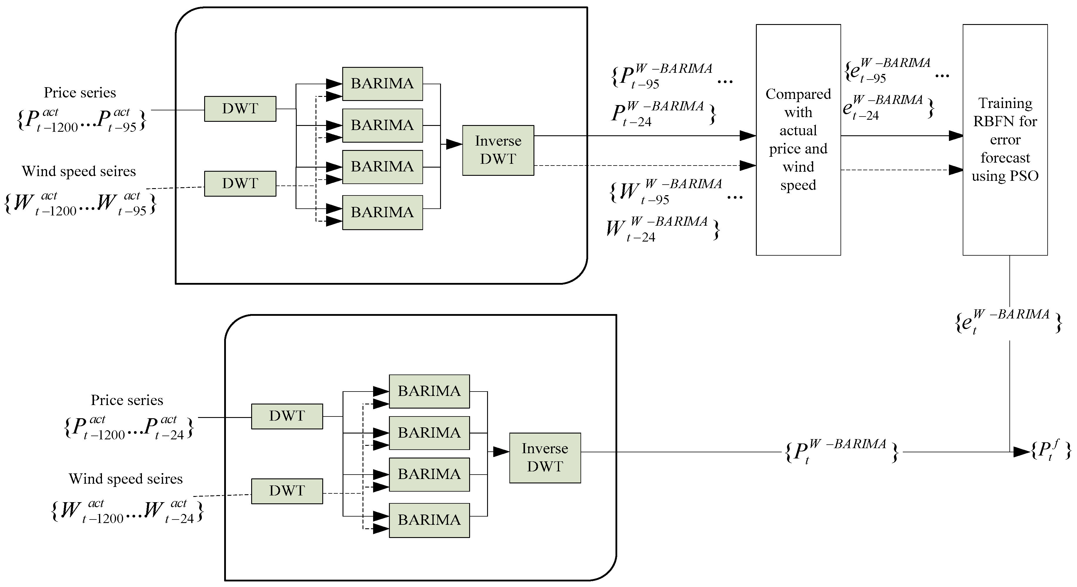
2. Proposed Electricity Market Prices Forecasting Method

2.1. Wavelet Transform

A WT is a mathematical tool for signal analysis. The key concept in Wavelet analysis is to select a proper wavelet called mother wavelet, such as Herr Wavelet, Meyer wavelet, Coiflet wavelet, Morlet wavelet. Then an analysis is performed using its translated and detailed version.

There are several WT such as continuous Wavelet Transform (CWT) which is also known as integral wavelet transform (IWT), DWT, and fast discrete wavelet transform (FWT) which is also known as multi-resolution analysis (MRA). CWT is defined as follows for a signal called f(t) [10,25]:

$$(W_f)(a,b)=a^{-\frac{1}{2}}{\displaystyle \underset{-\infty }{\overset{+\infty }{\int }}f(t)\psi (\frac{t-b}{a})dt}$$

(1)

where $\psi (t)$ is the mother Wavelet. The value of the WT $\left(W_f\right)\left(a,b\right)$ is known as Wavelet coefficient which stands for the similar degree between the signal and the Wavelet at the translation $b$, which means the time shift, and the dilation$a$, which means the time scale. In fact, it indicates how many components of wavelet at dilation $a$ are included in the original signal at translation $b$.

For computer performance, DWT is the most applied. Similar to fast Fourier transform (FFT), there is a fast algorithm for DWT called fast DWT.

In this method, an original discrete signal is decomposed into two components $c_1$ and $d_1$ through a low-pass filter and a high-pass filter, respectively. The aforementioned transformation is an orthogonal decomposition of signal and $c_1$ is approximation of signal which includes low frequency components and $d_1$ is the details of the signal related to high frequency components. Afterwards, $c_1$ is again decomposed into new approximation $c_2$ and new detail $d_2$ through a bigger scale. This procedure and decomposition can be done repeatedly, according to the application. The original signal can be also reconstructed through all approximations and details [7].

However, while FFT and WT are both domain transform functions, FFT has some disadvantages. The first is that frequency information is only able to be extracted for the complete duration of the signal. Another disadvantage is that the phase shift; both of these disadvantages can be overcome through WT. One of the other advantages of WT is adjusting of the window widths automatically. It means that in WT at low frequency, the window widths are longer and at high frequency the window widths are shorter, whereas both are fixed in the FFT. Therefore, WT can provide better time resolution for high frequency components and better frequency resolution for low-frequency components. Moreover, due to the shorter time-window, the phase shift is hardly observed [11].

In this work, two time series, including the time series for market price data and weighted time series for wind speed, are decomposed to some subseries through described DWT. After forecasting the procedure, all the forecasted volumes obtained from time series are converted to day-ahead market price through inverse DWT.

2.2. Radial Basis Function Neural Network (RBFN)

RBFN has three levels including input layer, hidden layer and output layer. Some of the advantages of RBFN in comparison with other neural network are the rapid training phase, the simple architecture and also maintaining complicating mapping abilities [7,25,26,27].

The input layer involves signal source nodes. The output layer has a linear feature; however, the hidden layer is nonlinear and its varying function is a radial basis function. The Gaussian function is mostly used as a basic function. Usually, the output node combines the outputs of the hidden nodes.

The learning procedure of RBFN includes two stages. In the first stage, unsupervised methods are used in the training of hidden layer to specify the centric value vectors of Gaussian basis function and weights from the input layer to the output layer. In the second stage, the output layer is trained via a supervised method to determine the weights from the hidden layer to the output layer [28].

2.3. Bivariate ARIMA-Wavelet and RBFN

There are two ARIMA models for price forecasting including univariate and multivariate models [29]. In the univariate model, using the historical electricity price variation, price forecasting is implemented [30]. However, in the multivariate model, in addition to price data, other variables are taken into account [31]. Interaction among electricity market prices and other variables of the power system, which are mostly economic indices such as fuel cost, is another application of this method.

Most of the multivariate models have been applied for long-term and mid-term forecasting; although this method has been utilized for short-term forecasting in this work. A bivariate model based on price series, as well as wind speed series for price forecasting, has been applied in this paper for price forecasting.

For stationary time series, ARMA is used, however in the case of any seasonal trend in the time series, the ARIMA model, which is the combination of MA and AR is applied. The general model of ARIMA is the ARIMA_(p,d,q), where p is the number of autoregressive terms, d is the degree of differencing to make the model stationary, and q is the number of moving average or lagged forecast error in the model.

ARIMA has three stages. First of all, the suitable model should be identified. In other words, the proper quantity of p, q and d should be determined in order to obtain a model that is worth further investigation. Second, parameters should be initially estimated and finally, the model should be checked to see it if it fits the data.

ARIMA models allow for each variable to be explained by historical data and error items. In this model, the deferential function is applied d times on time series to turn it into the stationary time series and then the ARMA model is applied. The univariable model of ARIMA is as follows [3,32]:

$$y_t={\theta }_0+{\phi }_1{y}_{t-1}+{\phi }_2{y}_{t-2}+\dots +{\phi }_p{y}_{t-p}+{\epsilon }_t-{\theta }_1{\epsilon }_{t-1}-{\theta }_2{\epsilon }_{t-2}-\dots -{\theta }_q{\epsilon }_{t-q}$$

(2)

where $\phi$ and $\theta$ are constant coefficients of variable and error, respectively. Moreover, y and $\epsilon$ are the variable and error variable. With this univariable ARIMA model, only the effect of past electricity price variables on electricity price, can be considered. In a wind generator dominated power system, the electricity market price depends remarkably on wind power production; therefore, in addition to past electricity market prices, the effect of prior wind speed volumes should be taken into account.

In other words, (2) is not suitable for our purpose because we want to have two variables including electricity price and wind speed in the prediction processor; however, (3) can be applied to forecast our proposed model. Accordingly, the BARIMA model has been considered as follows [32]:

$$\begin{array}{ll}{y}_t=& {\theta }_0+{\phi }_1^{(1)}{y}_{t-1}^{(1)}+{\phi }_2^{(1)}{y}_{t-2}^{(1)}+\dots +{\phi }_{p_1}^{(1)}{y}_{{t-p}_1}^{(1)}+{\phi }_1^{(2)}{y}_{t-1}^{(2)}+{\phi }_2^{(2)}{y}_{t-2}^{(2)}+\dots +{\phi }_{p_2}^{(2)}{y}_{t-p_2}^{(2)}\\ & +{\epsilon }_t-{\theta }_1{\epsilon }_{t-1}-{\theta }_2{\epsilon }_{t-2}-\dots -{\theta }_q{\epsilon }_{t-q}\end{array}$$

(3)

where the superscripts indicate the first variable (electricity market price) and second variable (wind speed). Since both of these time series are somewhat chaotic, and in this sense, it is required to decompose the time series into several more homogeneous subseries. The time series can be decomposed to three subseries [10], five [33], and up to seven subseries [34] depending on type and frequency of the variation. In this work, time series is decomposed into four subseries.

Hourly wind speed is not constant all over parts of the network. Moreover, the impact of wind speed on market price in the region with more wind power generators is remarkably higher. Since in this model, previous wind speeds should be considered as time series, it is proposed that prior wind speed data from different areas are weighted based on wind production capacity. It means the impact of wind power capacity in different parts of network on electricity price is taken into account via the weighting factor definition for wind power capacity in different regions. Wind speed weighting is presented in the following equations.

Equation (4) is the calculation of the capacity factor $K{w}_i$ in $i\mathrm{th}$ region of the power system with a specific capacity of wind power generators. According to (4), the capacity of power generator $Win{d}_i^{Cap}$ in $i\mathrm{th}$ region divided to total wind power capacity, which is the summation of all wind power generators capacity, ${{\displaystyle \sum }}_{i=1}^{WindNo}Win{d}_i^{Cap}$, which leads to obtaining the wind weighting $K{w}_i$ for each region $i$.

This coefficient is used in Equation (5) to multiply the wind speed data in a region at the specific time, $Win{d}_{i,t}$. The summation of this parameter for all regions leads to achieving actual wind speed time series for a time, $Win{d}_t^{act}$, which is used as an input for DWT, based on Figure 1.

$$K{w}_i=\frac{Win{d}_i^{Cap}}{{\displaystyle \sum _{i=1}^{WindNo}Win{d}_i^{Cap}}}$$

(4)

$$W_t^{act}={\displaystyle \sum _{i=1}^{WindNo}K{w}_i·Win{d}_{i,t}}$$

(5)

Accordingly, for each part of the power system with a wind generator, the time series related to wind speed is extracted. Afterwards, through Equations (4) and (5), a weighted time series for wind speed for the whole network has been calculated. Two time series including time series for market price data and weighted time series for wind speed are decomposed to some subseries through WT.

The all future volumes of electricity price in the subseries are predicted through the BARIMA method according to Equation (3). Finally, all these forecasted volumes obtained from time series are converted to the day-ahead market price through inverse DWT.

In this work, hourly wind speed and electricity market price data from four days (96 h) to fifty days (1200 h) before the current day (forecast time t) are applied as an input time series for WT, which decomposes the time series into three levels. Outputs of WT, which are four time series, go to ARIMA model for forecasting. ARIMA outputs are turned into forecasted prices and wind speed data through inverse WT for one day (24 h) to five days (96 h) before forecasting time t. Since this forecasting is for five days before current forecasting time, this information can be used for calculation of forecast error.

Therefore, the forecasted amount of W-BARIMA is compared with an actual one to estimate the forecast error and train the RBFN using PSO method. Afterwards, the forecast electricity price and wind speed at the forecast time t can be predicted using W-BARIMA-RBFN method and data from fifty days (1200 h) to 24 h before the forecast time t.

Moreover, according to Figure 1, the proposed methodology consists of two main parts. The first part (upper part in Figure 1) is for the calculation of forecast error. In this part, time series of price and wind speed from data ranging from fifty days to five days prior are decomposed to four subseries through BARIMA, and after forecasting procedure, the wind speed price time series from five day to 1 day before prediction time are obtained, separately.

These predicted data are compared with the actual data to achieve the forecast error of the method and train the RBFN. The output of this part is the error of the forecasting method, which is used in the second part (lower part in Figure 1). Indeed, in the second part, the forecasting for the prediction time is conducted through time series of electricity price and wind speed from the data ranging from fifty days to one day prior prediction time. After the forecasting procedure, the output is corrected by the forecast error obtained in the first part.

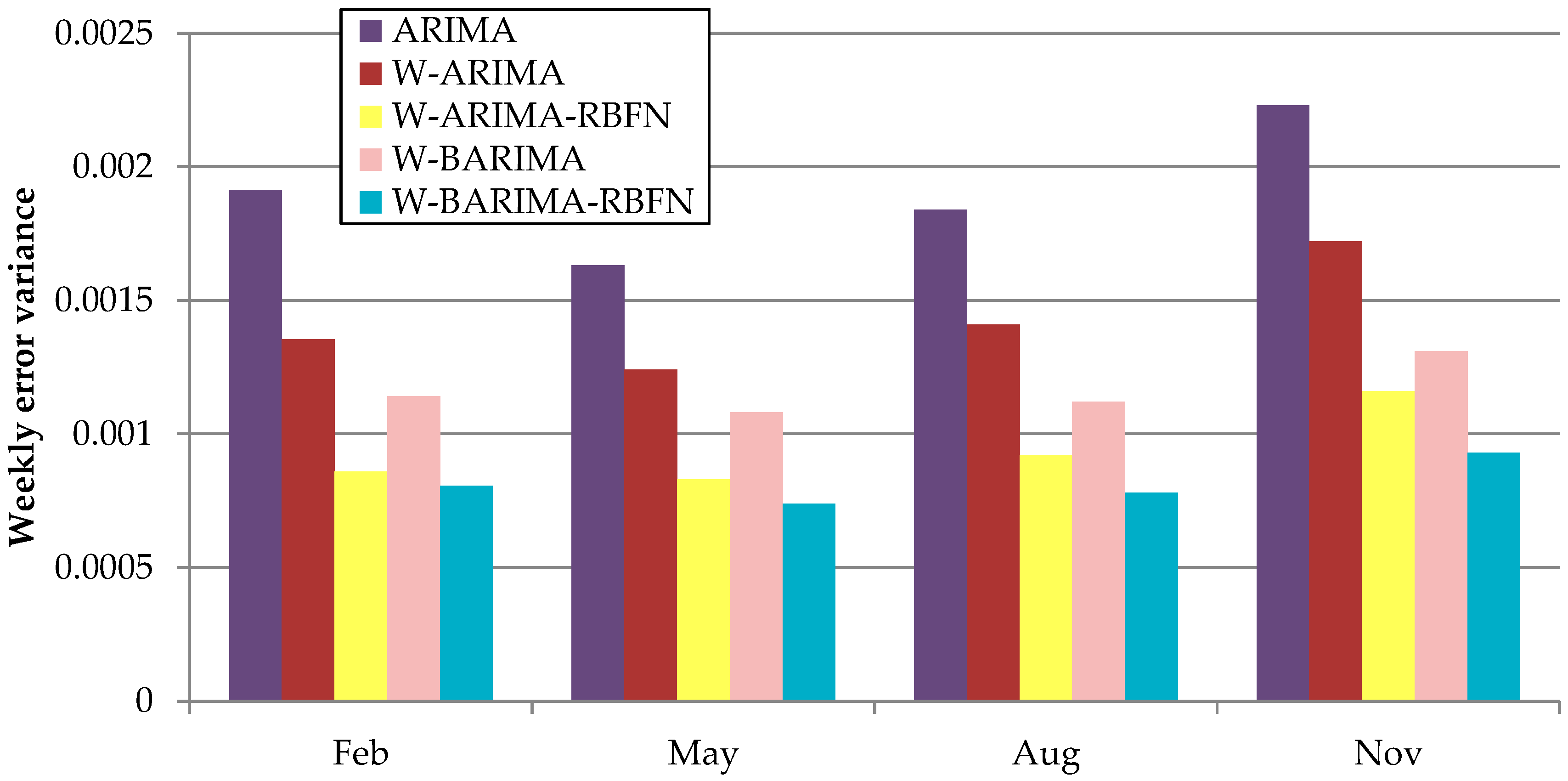
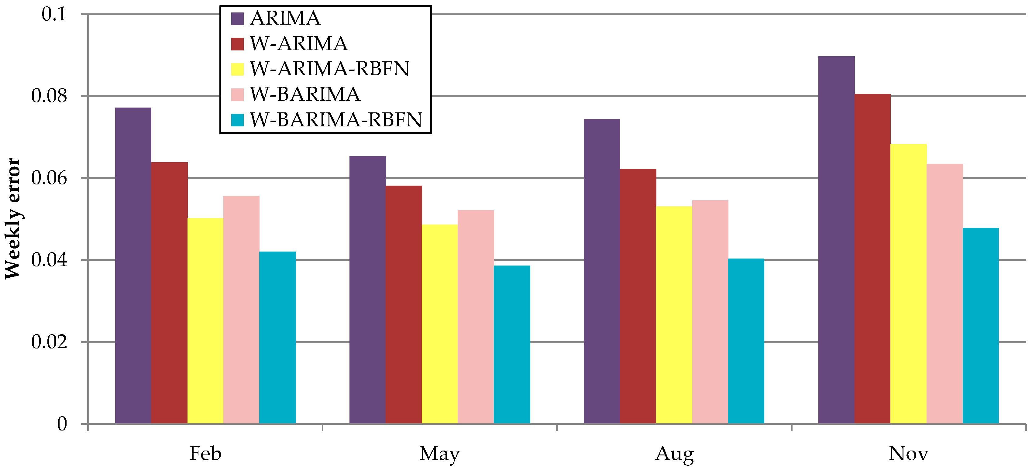
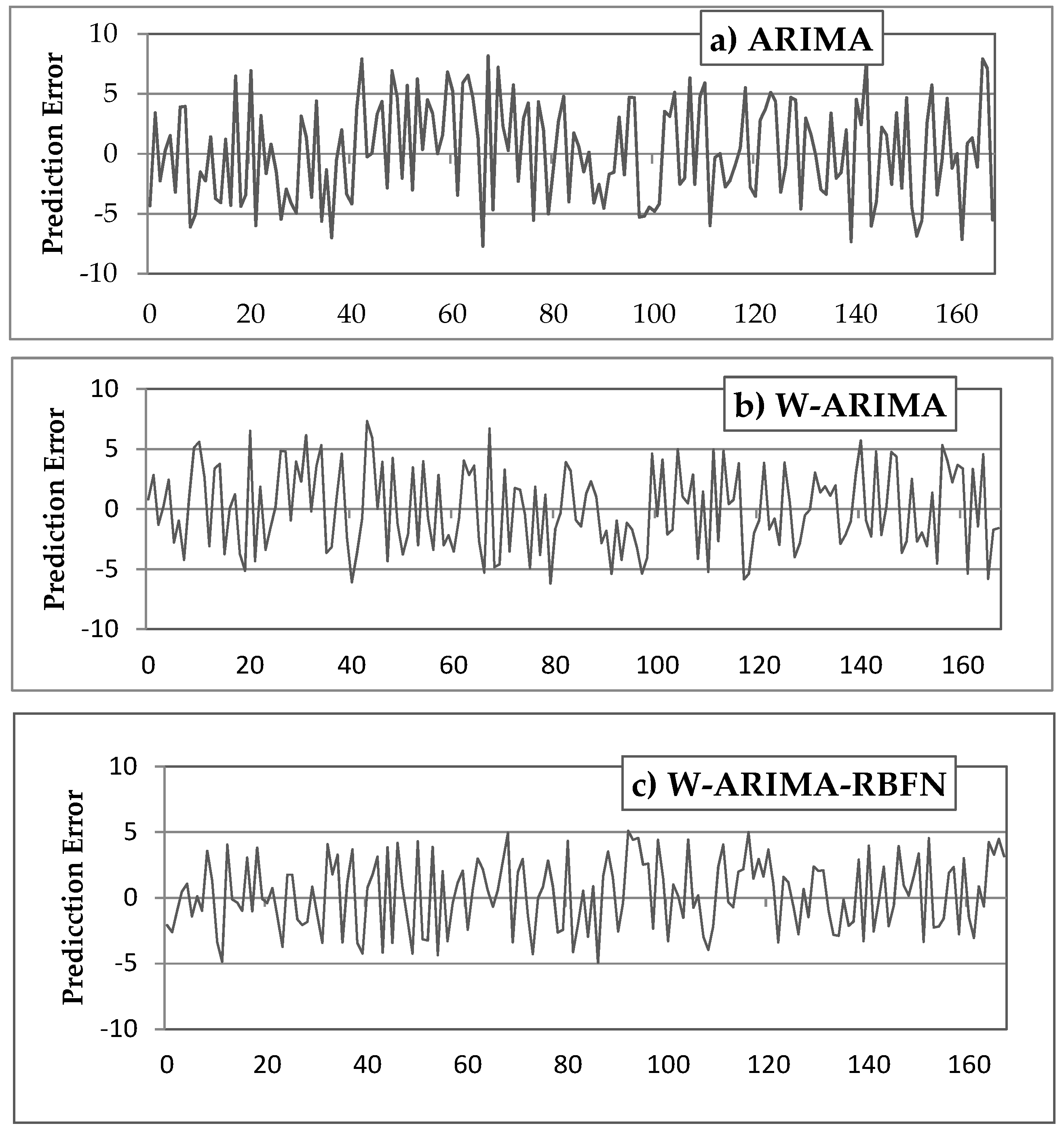
3. Prediction Accuracy

To evaluate the accuracy of this W-BARIMA, three indices for error prediction, including hourly error, 168 h weekly error and weekly error variance are computed. Per unit, weekly error can be calculated as follows [8]:

$$e_{week}=\frac{1}{168}{\displaystyle \sum _{h=1}^{168}\frac{\left|P_h^{true}-P_h^{est}\right|}{{\overline{P}}_{week}^{true}}}$$

(6)

where:

$${\overline{P}}_{week}^{true}=\frac{1}{168}{\displaystyle \sum _{h=1}^{168}{P}_h^{true}}$$

(7)

Weekly variance error can be calculated as follows:

$${\sigma }_{e,week}^2=\frac{1}{168}{{\displaystyle \sum _{h=1}^{168}\left(\frac{\left|P_h^{true}-P_h^{est}\right|}{{\overline{P}}_{168}^{true}}-\left(e_{week}\right)\right)}}^2$$

(8)

4. Numerical Study

The proposed method, W-BARIMA-RBFN is implemented on the mainland electricity Spain market for four weeks in order to assess the capability and accuracy of the model. This method, without considering RBFN, is performed as well to show the impact of RBFN. Moreover, the comparison among the proposed method and other forecasting models, including ARIMA, W-ARIMA, W-ARIMA-RBFN and W-BARIMA, is conducted. Each week is related to a season.

The first week is associated with Winter 22 to 28 February, the second week is respect to Spring 25 to 31 May, the third week is regarding Summer 25 to 31 August and the fourth week is related to Autumn 24 to 30 November.

For the electricity price forecasting in winter, the hourly electricity market and wind speed for the past fifty days are required. For example, for electricity price forecasting on 22 February, hourly electricity prices and wind speed from 3 January to 21 February are needed. Comparison with actual data and predicted ones, the merit of the proposed forecasting method are assessed. Hourly electricity price from [35] and wind speed data from [36] are extracted.

Spain’s power system consists of more than 20,000 MW wind power capacity, which is 20 percent of Spain’s total power production capacity. In this work, to generate weighted wind series, only wind power producers with a capacity of more than 300 MW are considered and the impact of other smaller wind power producers (wind power operators) on electricity price is neglected. The reason why only more than 300 MW wind farms are selected, is that smaller-scale ones have lower impact on wind speed wind weighting $K{w}_i$ and the focus of this study is on the transmission level. Hence, eight wind power producers in different Spain’s regions are considered

Table 1. Spain’s wind power generators data.

Region	Capacity (MW)	$\mathit{K}{\mathit{w}}_{\mathit{i}}$	Average Wind Speed (Knot)
			February	May	August	November
Galicia	3238	0.172	7	9	6	6
Navarra	976	0.052	3	5	5	5
Asturias	414	0.022	8	7	7	8
Aragon	1751	0.093	2	4	3	3
Castilla y Leon	4540	0.241	10	7	8	9
Castilla la Mancha	3761	0.199	5	7	6	6
C. Valenciana	1174	0.062	3	4	4	4
Andalucia	2993	0.159	5	6	5	5

.

Based on Table 1, the wind speed in Castilla y Leon has the most effect on the weighted wind series. A comparison of forecasting results among the proposed method (W-BARIMA-RBFN) and other methods including ARIMA [3], W-ARIMA [10], W-ARIMA-RBFN [8], W-BARIMA and W-BARIMA-RBFN are shown in Figure 2. Moreover, another comparison for weekly error and weekly error variance between the proposed method and other methods are demonstrated in Figure 3 and Figure 4, respectively.

According to the results, weekly error and weekly error variance for W-BARIMA is less than ARIMA and W-ARIMA. However, the weekly error variance of W-BARIMA for all 4 months and weekly error of W-BARIMA for February, May and August is more than W-ARIMA-RBFN BARIMA.

Moreover, all errors of the proposed method, W-BARIMA-RBFN, for all seasons are, overall, less than other methods analyzed. Therefore, performing the W-BARIMA is not enough to have an accurate price forecasting, and RBFN should be applied to reduce the forecasting errors.

In Figure 5, a comparison of various forecasting methods is conducted to show the difference between the actual electricity price and the forecasted one. Accordingly, the proposed method has the lowest difference among actual and forecasted price.

Furthermore, in Figure 6, the variance of different forecasting methods is demonstrated. As can be seen, ARIMA has the worst, and the proposed method has the best situation, in these figures.

5. Conclusions

In this paper, a hybrid method has been utilized to forecast day-ahead prices in a competitive electricity market with high penetration of wind power generation. In the proposed methodology, a combination of Wavelet transform, bivariate ARIMA, and RBFN has been applied. In addition to past electricity price data, prior wind speed data has been added as a second variable to the ARIMA method as well. One of the merits of the proposed model is to consider the effects of large-scale wind generators on electricity prices through the bivariate ARIMA; therefore, it is useful indeed for modern electricity markets that have many wind generators. Moreover, adding the RBFN method to W-BARIMA has a remarkable impact on decreasing forecasting errors, achieving more accurate results as compared with other methods. For future work, considering the uncertainty analysis and small-scale wind farms would serve as significant contributions to the research field.

References

1. Shahidehpour, M.; Yamin, H.; Li, Z. Market Operations in Electric Power Systems: Forecasting, Scheduling, and Risk Management; Institute of Electrical and Electronics Engineers, Wiley-Interscience: New York, NY, USA, 2002; ISBN 978-0-471-44337-7. [Google Scholar]
2. Crespo Cuaresma, J.; Hlouskova, J.; Kossmeier, S.; Obersteiner, M. Forecasting electricity spot-prices using linear univariate time-series models. Appl. Energy 2004, 77, 87–106. [Google Scholar] [CrossRef]
3. Contreras, J.; Espinola, R.; Nogales, F.J.; Conejo, A.J. ARIMA models to predict next-day electricity prices. IEEE Trans. Power Syst. 2003, 18, 1014–1020. [Google Scholar] [CrossRef]
4. Garcia, R.C.; Contreras, J.; Akkeren, M.; van Garcia, J.B.C. A GARCH forecasting model to predict day-ahead electricity prices. IEEE Trans. Power Syst. 2005, 20, 867–874. [Google Scholar] [CrossRef]
5. MateoGonzalez, A.; MunozSanRoque, A.; Garcia-Gonzalez, J. Modeling and Forecasting Electricity Prices with Input/Output Hidden Markov Models. IEEE Trans. Power Syst. 2005, 20, 13–24. [Google Scholar] [CrossRef]
6. Kim, C.; Yu, I.-K.; Song, Y.H. Prediction of system marginal price of electricity using wavelet transform analysis. Energy Convers. Manag. 2002, 43, 1839–1851. [Google Scholar] [CrossRef]
7. Yao, S.J.; Song, Y.H.; Zhang, L.Z.; Cheng, X.Y. Prediction of System Marginal Prices by Wavelet Transform and Neural Networks. Electr. Mach. Power Syst. 2000, 28, 983–993. [Google Scholar] [CrossRef]
8. Shafie-khah, M.; Moghaddam, M.P.; Sheikh-El-Eslami, M.K. Price forecasting of day-ahead electricity markets using a hybrid forecast method. Energy Convers. Manag. 2011, 52, 2165–2169. [Google Scholar] [CrossRef]
9. Huang, C.-M.; Huang, C.-J.; Wang, M.-L. A particle swarm optimization to identifying the ARMAX model for short-term load forecasting. IEEE Trans. Power Syst. 2005, 20, 1126–1133. [Google Scholar] [CrossRef]
10. Conejo, A.J.; Plazas, M.A.; Espinola, R.; Molina, A.B. Day-Ahead Electricity Price Forecasting Using the Wavelet Transform and ARIMA Models. IEEE Trans. Power Syst. 2005, 20, 1035–1042. [Google Scholar] [CrossRef]
11. Tan, Z.; Zhang, J.; Wang, J.; Xu, J. Day-ahead electricity price forecasting using wavelet transform combined with ARIMA and GARCH models. Appl. Energy 2010, 87, 3606–3610. [Google Scholar] [CrossRef]
12. Amjady, N.; Hemmati, M. Energy price forecasting-problems and proposals for such predictions. IEEE Power Energy Mag. 2006, 4, 20–29. [Google Scholar] [CrossRef]
13. Amjady, N. Day-Ahead Price Forecasting of Electricity Markets by a New Fuzzy Neural Network. IEEE Trans. Power Syst. 2006, 21, 887–896. [Google Scholar] [CrossRef]
14. Catalão, J.P.S.; Mariano, S.J.P.S.; Mendes, V.M.F.; Ferreira, L.A.F.M. Short-term electricity prices forecasting in a competitive market: A neural network approach. Electr. Power Syst. Res. 2007, 77, 1297–1304. [Google Scholar] [CrossRef]
15. Wang, A.J.; Ramsay, B. A neural network based estimator for electricity spot-pricing with particular reference to weekend and public holidays. Neurocomputing 1998, 23, 47–57. [Google Scholar] [CrossRef]
16. Szkuta, B.R.; Sanabria, L.A.; Dillon, T.S. Electricity price short-term forecasting using artificial neural networks. IEEE Trans. Power Syst. 1999, 14, 851–857. [Google Scholar] [CrossRef]
17. Gao, F.; Guan, X.; Cao, X.-R.; Papalexopoulos, A. Forecasting power market clearing price and quantity using a neural network method. In Proceedings of the 2000 Power Engineering Society Summer Meeting, Seattle, WA, USA, 16–20 July 2000; Volume 4, pp. 2183–2188. [Google Scholar]
18. Hong, Y.Y.; Hsiao, C.Y. Locational marginal price forecasting in deregulated electricity markets using artificial intelligence. IEE Proc. Gener. Transm. Distrib. 2002, 149, 621–626. [Google Scholar] [CrossRef]
19. Zhang, L.; Luh, P.B. Power market clearing price prediction and confidence interval estimation with fast neural network learning. In Proceedings of the 2002 IEEE Power Engineering Society Winter Meeting, New York, NY, USA, 27–31 January 2002; Volume 1, pp. 268–273. [Google Scholar]
20. Rodriguez, C.P.; Anders, G.J. Energy price forecasting in the Ontario competitive power system market. IEEE Trans. Power Syst. 2004, 19, 366–374. [Google Scholar] [CrossRef]
21. Bunn, D.W. Forecasting loads and prices in competitive power markets. Proc. IEEE 2000, 88, 163–169. [Google Scholar] [CrossRef]
22. Jalili, A.; Ghadimi, N. Hybrid harmony search algorithm and fuzzy mechanism for solving congestion management problem in an electricity market. Complexity 2016, 21, 90–98. [Google Scholar] [CrossRef]
23. Hosseini, F.M.; Ghadimi, N. Optimal preventive maintenance policy for electric power distribution systems based on the fuzzy AHP methods. Complexity 2016, 21, 70–88. [Google Scholar] [CrossRef]
24. Guo, J.-J.; Luh, P.B. Improving market clearing price prediction by using a committee machine of neural networks. IEEE Trans. Power Syst. 2004, 19, 1867–1876. [Google Scholar] [CrossRef]
25. Olamaee, J.; Mohammadi, M.; Noruzi, A.; Hosseini, S.M.H. Day-ahead price forecasting based on hybrid prediction model. Complexity 2016, 21, 156–164. [Google Scholar] [CrossRef]
26. Zhang, L.; Luh, P.B. Neural network-based market clearing price prediction and confidence interval estimation with an improved extended Kalman filter method. IEEE Trans. Power Syst. 2005, 20, 59–66. [Google Scholar] [CrossRef]
27. Hong, Y.Y.; Hsiao, C.-Y. Locational marginal price forecasting in deregulated electric markets using a recurrent neural network. In Proceedings of the 2001 IEEE Power Engineering Society Winter Meeting, Columbus, OH, USA, 28 January–1 February 2001; Volume 2, pp. 539–544. [Google Scholar]
28. Zhang, K.; Shi, Q. Power Futures Price Forecasting Based on RBF Neural Network. In Proceedings of the 2009 International Conference on Business Intelligence and Financial Engineering, Beijing, China, 24–26 July 2009; pp. 50–52. [Google Scholar]
29. Weron, R. Electricity price forecasting: A review of the state-of-the-art with a look into the future. Int. J. Forecast. 2014, 30, 1030–1081. [Google Scholar] [CrossRef]
30. Aggarwal, S.K.; Saini, L.M.; Kumar, A. Electricity price forecasting in deregulated markets: A review and evaluation. Int. J. Electr. Power Energy Syst. 2009, 31, 13–22. [Google Scholar] [CrossRef]
31. Cadenas, E.; Rivera, W.; Campos-Amezcua, R.; Heard, C. Wind Speed Prediction Using a Univariate ARIMA Model and a Multivariate NARX Model. Energies 2016, 9, 109. [Google Scholar] [CrossRef]
32. Zhang, G.P. Time series forecasting using a hybrid ARIMA and neural network model. Neurocomputing 2003, 50, 159–175. [Google Scholar] [CrossRef]
33. Yousefi, S.; Weinreich, I.; Reinarz, D. Wavelet-based prediction of oil prices. Chaos Solitons Fractals 2005, 25, 265–275. [Google Scholar] [CrossRef]
34. Fernandez, V. Wavelet- and SVM-based forecasts: An analysis of the U.S. metal and materials manufacturing industry. Resour. Policy 2007, 32, 80–89. [Google Scholar] [CrossRef]
35. Inicio. Ontology Mapping within an Interactive and Extensible Environment (OMIE). Available online: http://www.omie.es/en/inicio (accessed on 24 August 2017).
36. Windfinder.com. Windfinder—Wind, Wave & Weather Reports, Forecasts & Statistics Worldwide. Available online: https://www.windfinder.com (accessed on 25 August 2017).
Figure 1. Proposed method for electricity price forecasting.
Sustainability 09 02065 g001
Figure 2. Comparison price forecasting results among Wavelet Transform Bivariate Auto-Regressive Integrated Moving Average Radial Basis Function Neural Network (W-BARIMA-RBFN) method and other methods.
Sustainability 09 02065 g002
Figure 3. Comparison weekly error results among W-BARIMA-RBFN method and other methods.
Sustainability 09 02065 g003
Figure 4. Comparison weekly error results among W-BARIMA-RBFN method and other methods.
Sustainability 09 02065 g004
Figure 5. Difference between the actual and forecasted amount of electricity price in various methods. (a) Auto-Regressive Integrated Moving Average (ARIMA) method; (b) Wavelet Transform Auto-Regressive Integrated Moving Average (W-ARIMA); (c) Wavelet Transform Auto-Regressive Integrated Moving Average Radial Basis Function Neural Network (W-ARIMA-RBFN); (d) Wavelet Transform Bivariate Auto-Regressive Integrated Moving Average (W-BARIMA); (e) W-BARIMA-RBFN.
Sustainability 09 02065 g005aSustainability 09 02065 g005b
Figure 6. Variance for different forecasting method (a) ARIMA; (b) W-ARIMA; (c) W-ARIMA-RBFN; (d) W-BARIMA; (e) W-BARIMA-RBFN.
Sustainability 09 02065 g006aSustainability 09 02065 g006b