Undisturbed Ground Temperature—Different Methods of Determination

Abstract

Methods for the calculation of the undisturbed ground temperature (UGT) are presented. Heat fluxes occurring on the surface of the ground and their influence on the UGT are described. Correlation equations for the calculation of the undisturbed ground temperature based on the meteorological data averaged in the yearly cycle are proposed. These equations are of a semi-empirical character and they are based on the heat flux balance. The determined coefficients of these equations, particularly the convection heat transfer coefficient, are consistent with the values specified by other methods.

1. Introduction

The undisturbed ground temperature (UGT) is an important parameter while designing, modelling, and using ground heat exchangers and other equipment connected with heat transport in the ground (e.g., conduits transporting heat carriers). The ground may be considered as a complex system that consists of a subsurface layer, experiencing interactions with variable atmospheric conditions, and a deeper layer having no such interactions. Starting from a certain distance from the surface, the ground temperature is approximately stable. Slight changes in the ground temperature below the depth at which the influence of atmospheric conditions fades result from the existence of the geothermal flux. However, its effect on the operation of ground heat exchangers (GHE) is usually omitted. The UGT depends on climatic conditions and is different in various regions of the Earth. The average UGT value on the Earth should be identified with the average temperature of the Earth’s surface, estimated as ca. 15 °C.

Ground temperature in the subsurface layer depends on location and time [1]. The thickness of this layer depends on the thermal diffusivity of the ground. For low values of thermal diffusivity the subsurface layer has a small thickness, but when the thermal diffusivity of the ground is high, the stabilisation of the ground temperature occurs at larger depths. Most often, the depths of subsurface layers, depending on the thermal properties of the ground, are in the range of 8 to 18 m. Due to the thermal inertia of the ground, the amplitude of changes in the ground temperature decreases with an increasing depth. The amplitude of changes in the ground temperature caused by diurnal temperature changes on the surface decreases to zero at a depth of ca. 1 m, while the amplitude caused by seasonal changes decreases with increasing distance from the surface of the ground to a significantly lesser degree.

For the zero geothermal gradient, the values of the UGT and the average temperature of the surface of the ground are identical. The values of the geothermal gradient actually occurring in nature affect the diversification of these temperatures only slightly. The temperature difference between the levels of the ground separated by 10 m, caused by this gradient, is of the order of 0.3 K, assuming an average value of the geothermal gradient of 0.03 K/m acc. to Al-Khoury [2]. Thus, the equality of the average temperature of the ground surface and the UGT under typical conditions may be generally assumed.

While designing equipment for heat extraction from the ground, the UGT value plays an important role, because the amount of heat that may be extracted is proportional to the difference between the UGT and the minimum temperature of the working liquid (resulting from its freezing temperature) [3]. If, while designing ground heat exchangers (GHE), yearly average ambient temperature is assumed as an approximation of the UGT value, it may lead to unjustified oversizing of the exchanger (when used for heating purposes) [4].

The magnitude of the UGT may be determined experimentally. Most often, the measurements are conducted using equipment for the Transient Response Test (TRT) [5,6]. While determining the temperature profile in the ground, a circulation of the working liquid through a Borehole Heat Exchanger is carried out without heating the liquid, and the temperature of the liquid at the borehole outlet is measured. Assuming that the liquid flow is a piston flow, the values of the liquid temperature at the borehole outlet may be considered as ones corresponding to temperatures at various depths in the ground. Another method for the determination of the temperature profile in the ground consists in the introduction of temperature sensors at various depths into a filled (e.g., with a liquid) U-tube of the exchanger, which was described in papers by, among others, Yu et al. [7] and Zhou et al. [8].

Experimental determination of thermal parameters of the ground constituted the subject of numerous studies. Kusuda and Achenbach [9] developed extensive experimental material concerning measurements of the ground temperature at various ground depths, conducted at 63 measurement stations in the USA. The parameters of the proposed mathematical model included the UGT. Similar measurement results for a single measurement station are presented, among others, in paper [10]. Also, publications in which the observations from weather stations were correlated with meteorological parameters concerned the determination of the UGT. Recently, works concerning the UGT were reported by Ouzzane et al. [4,11] and Badache et al. [12].

In this paper, the heat flux balance on the surface of the ground is related with correlation equations for determination of the UGT. Semi-empirical equations for calculation of the UGT, based on the balance of these fluxes, are proposed. Considerable attention was paid to the heat flux connected with evaporation of water from the surface of the ground (simultaneous heat and mass transfer).

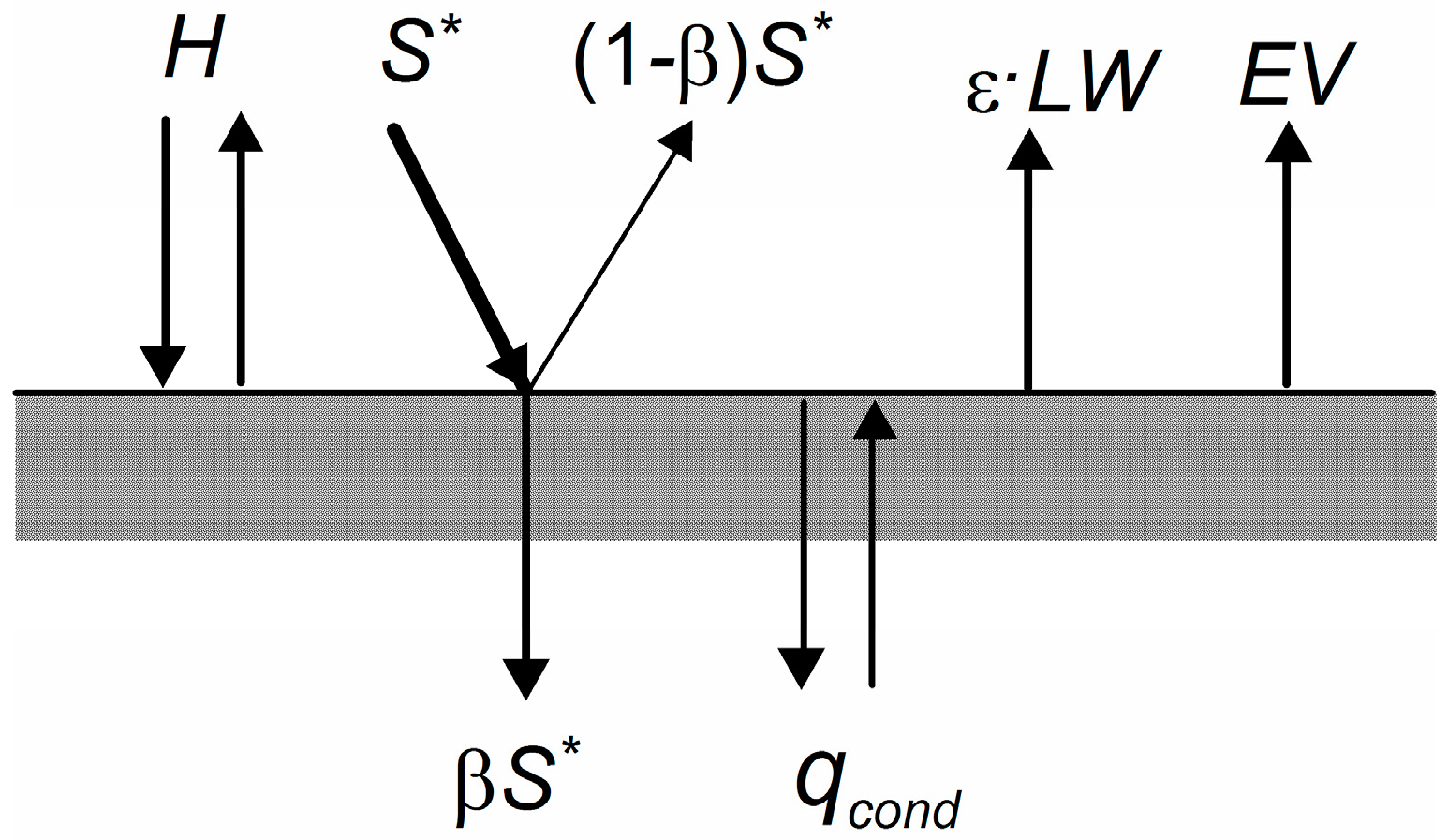
2. Heat Balance on the Surface of the Ground

The following heat fluxes exist on the surface of the ground: convective heat flux H, solar energy absorbed by the ground S = βS*, long-wave radiation heat flux ε·LW, and a flux caused by the evaporation of water contained in the ground EV (Figure 1). Horizontal solar radiation S* reaches the surface of the ground; a part of this flux is absorbed by the ground, and the other part is reflected from the surface of the ground. Irrespective of the reflected flux, the ground radiates heat towards the sky. Also, the ground loses heat as a result of the moisture evaporation. The heat flux resulting from an algebraic summation of the listed fluxes q_cond is transported into the ground (mainly by conduction) or in the opposite direction, depending on its minus/plus sign.

The heat balance on the surface of the ground taking into account convection, radiation, and moisture evaporation has the following form [13,14,15,16,17,18,19,20,21]:

$$-k{\left(\frac{\partial T}{\partial x}\right)}_{x=0}=q_{cond}=H+S-\epsilon \cdot LW-EV$$

(1)

The flux of heat conducted from the surface of the ground to its deeper layers is compensated by a heat flux in the opposite direction during yearly cycles (this fact being a requirement for the existence of a cyclic steady state). Thus, under natural conditions, the yearly average flux conducted via the ground amounts to:

$$\langle -k{\left(\frac{\partial T}{\partial x}\right)}_{x=0}\rangle =0$$

(2)

Assuming that the convection heat transfer coefficient h between the surface of the ground and the environment is constant in time, the yearly average convective flux amounts to:

$$\langle H\rangle =\langle h_{}\left(T_a-T_s\right)\rangle =\frac{1}{t_c}{\displaystyle \underset{0}{\overset{t_c}{\int }}h\left(T_a-T_s\right)}dt=h\left(\frac{1}{t_c}{\displaystyle \underset{0}{\overset{t_c}{\int }}{T}_a}dt-\frac{1}{t_c}{\displaystyle \underset{0}{\overset{t_c}{\int }}{T}_{s}dt}\right)=h\left(\langle T_a\rangle -\langle T_s\rangle \right)$$

(3)

where T_a—ambient temperature [°C], T_s—temperature of ground surface [°C], t_c—cycle time (=365 days), $\langle \dots \rangle$—yearly average value.

2.1. Solar Radiation and Long-Wave Radiation

The solar radiation flux is strongly variable in time: it has a zero value in the night and it is significantly higher during summer months than during winter months. In balance calculations, it is convenient to use the daily average density of this flux. Such values include the total solar radiation, both direct and scattered. The solar radiation flux reaching the surface of the ground S* or the flux absorbed by the ground S may be used. The dependence between those quantities is as follows:

$$S=\beta S^{*}$$

(4)

where the β coefficient takes into account the degree of the radiation absorption by the ground. The reflection coefficient (albedo, 1 − β) for the ground depends on the ground’s humidity and cover type. Values of the albedo for the typical materials are: asphalt 0.12, concrete 0.20, bare soil 0.15 [15].

The long-wave radiation flux LW amounts to:

$$LW=\sigma \left(T_s^4-T_{sky}^4\right)$$

(5)

where σ = 5.67 × 10⁻⁸ W/(m²K⁴). The sky temperature T_sky depends on the temperature of air and its humidity; moreover, it is variable during the day and night. The possibilities to determine it include the use of the empirical formula [22,23]:

$$T_{sky}=T_a{\left[0.711+0.0056T_{dp}+0.000073T_{dp}^2+0.013\cdot \cos \left(15t\right)\right]}^{1/4}$$

(6)

where T_dp is a dew point temperature in Celsius degrees, T_sky and T_a are expressed in Kelvins, while t is time measured since midnight expressed in hours. Approximately, the yearly average value of T_sky amounts to:

$$\langle T_{sky}\rangle \cong \langle T_a\rangle {\left(0.711+0.0056\langle T_{dp}\rangle +0.000073{\langle T_{dp}\rangle }^2\right)}^{1/4}$$

(7)

while the yearly average value of the long-wave radiation flux amounts to:

$$\langle LW\rangle \cong 4\sigma T_{LWm}^3\left(\langle T_s\rangle -\langle T_{sky}\rangle \right)$$

(8)

where T_LWm is an arithmetic mean of the $\langle T_s\rangle$ and $\langle T_{sky}\rangle$ values:

$$T_{LWm}=0.5\left(\langle T_s\rangle +\langle T_{sky}\rangle \right)$$

It is assumed in the approximate calculations that the average long-wave radiation flux amounts to 63 W/m² (in the direction from the surface of the ground) [13,24].

2.2. Evaporation of Water from the Surface of the Ground

Apart from convective and radiation fluxes, the heat is transported between the surface of the ground and the environment as a result of the evaporation of water contained in the ground.

The evaporation of water from the ground should be considered as a process of simultaneous heat and mass transfer. The stream of moisture is caused by a difference in the partial pressures of water vapour on the surface of the ground p_i and in the bulk of the gaseous phase p. This mass flux is connected with the heat flux transfer that is required for the evaporation of water, the heat being lost by the ground. This heat flux amounts to [25]:

$$EV=f{k}_p\left(p_i-p\right)L_{evap}$$

(9)

where k_p is a convective mass transfer coefficient, and L_evap—heat of evaporation of water. The evaporation rate parameter f takes into account the fact that the evaporation rate of water from the surface of the ground is lower than the evaporation rate from the water surface; this coefficient ranges from 0.1 ÷ 0.2 for dry soils to 0.4 ÷ 0.5 for humid soils. The Chilton-Colburn analogy of heat and mass transfer [26] leads to a dependence between the coefficients of heat and mass transfer, resulting in the following relation:

$$EV=Afh\left(p_i-p\right)$$

(10)

where A = 0.0168 K/Pa [13].

The p_i quantity is the saturated vapour pressure at a temperature of the surface of the ground (=P_sat,s), and p = RH·P_sat,a. The saturated vapour pressure is a non-linear function of temperature. In paper [13], a linear form of this relation was adopted: P_sat = a₁T + b₁. Therefore:

$$\langle EV\rangle =0.0168fh\left[\left(a_1\cdot \langle T_s\rangle +b_1\right)-RH\cdot \left(a_1\cdot \langle T_a\rangle +b_1\right)\right]$$

(11)

In this paper, the dependence of the pressure of saturated water vapour on the temperature is described by the quadratic function:

$$P_{sat}=a_2{T}^2+b_{2}T+c_2\hspace{1em}\left[\mathrm{Pa}\right]$$

(12)

On the basis of the values of saturated water vapour depending on the temperature [27] for the temperature range from 0 °C to 30 °C the values of constants in the Equation (12) were determined: a₂ = 3.21, b₂ = 24.7, c₂ = 611. The yearly average value of the saturated vapour pressure amounts to:

$$\langle P_{sat}\rangle =\frac{1}{t_c}{\displaystyle \underset{0}{\overset{t_c}{\int }}\left(a_2{T}^2+b_{2}T+c_2\right)}dt$$

(13)

while the temperature T is variable in time in the yearly cycle with an amplitude A. After integration:

$$\langle P_{sat}\rangle =c_2+b_2\langle T\rangle +a_2\left({\langle T\rangle }^2+\frac{A_{}^2}{2}\right)$$

(14)

For calculations of the yearly average flux value EV, an averaged value of the saturated vapour pressure was assumed, at the temperature of the surface of the ground (P_sat,s) and at the ambient temperature (P_sat,a), respectively:

$$\langle EV\rangle =Afh\left(\langle P_{sat,s}\rangle -RH\langle P_{sat,a}\rangle \right)$$

(15)

where RH—relative humidity of the ambient air.

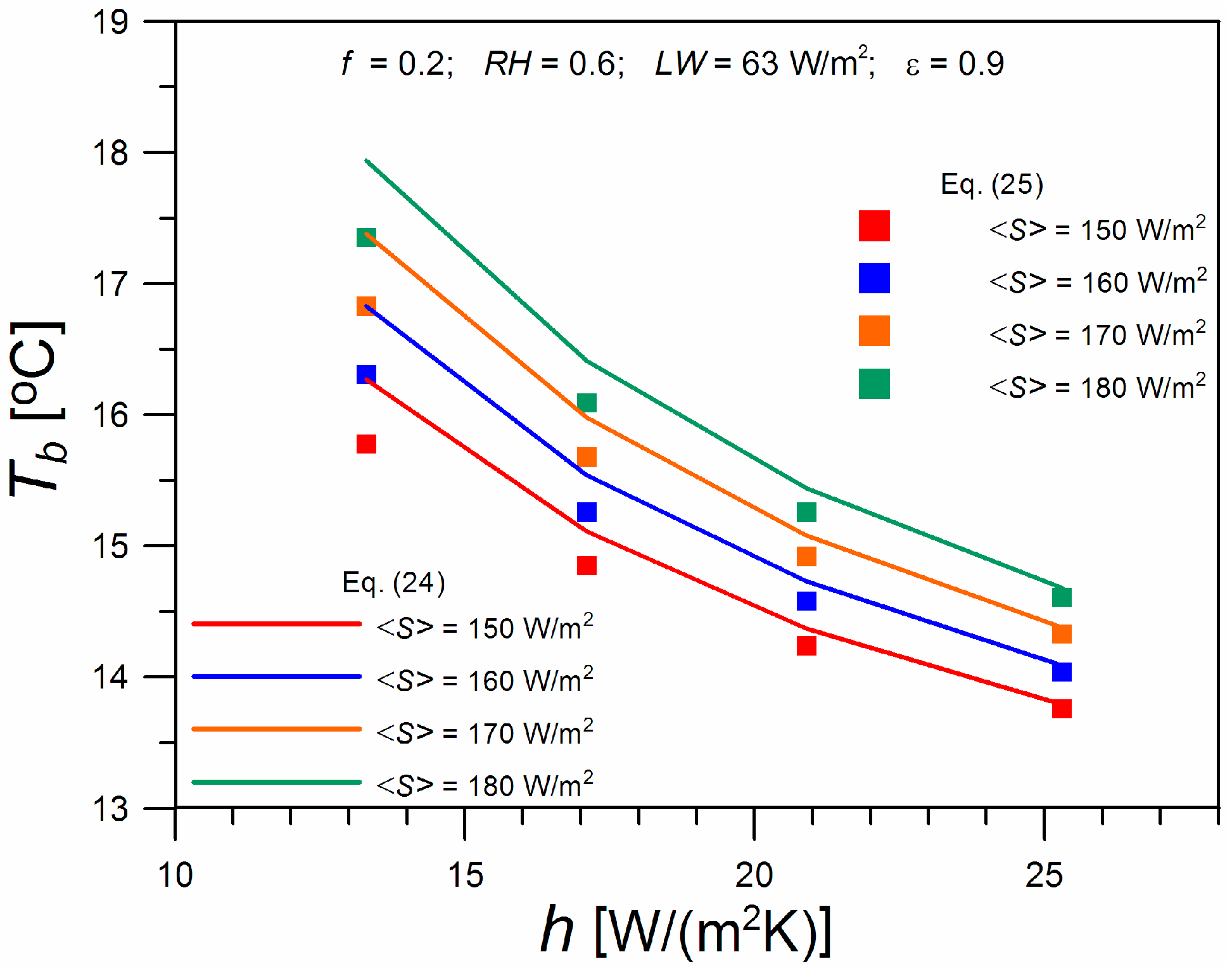
2.3. Results of Calculations

As $\langle T_s\rangle$ = T_b, so it results from the Formula (3) that:

$$T_b=\langle T_a\rangle -\frac{\langle H\rangle }{h}$$

(16)

Taking into account the values of heat fluxes averaged in the yearly cycle, the yearly average convective flux results from Equations (1) and (2):

$$\langle H\rangle =-\left(\langle S\rangle -\epsilon \cdot \langle LW\rangle -\langle EV\rangle \right)$$

(17)

Therefore, the UGT value may be determined using the following dependence:

$$T_b=\langle T_a\rangle +\frac{\langle S\rangle -\epsilon \cdot \langle LW\rangle -\langle EV\rangle }{h}$$

(18)

The convective heat transfer coefficients between the surface of the ground and the environment are difficult to determine precisely; various empirical dependencies are used for their determination. Frequently, the McAdams formula [28] is used, making this coefficient dependent on the wind velocity u:

$$\begin{array}{l}h=5.7+3.8u\hspace{0.17em}\hspace{1em}\hspace{1em}\mathrm{for}\hspace{1em}\hspace{1em}u<4.88\hspace{0.17em}\mathrm{m}/\mathrm{s}\hspace{0.17em}\\ h=7.2\hspace{0.17em}{u}^{0.78}\hspace{1em}\hspace{1em}\hspace{1em}\mathrm{for}\hspace{1em}\hspace{1em}u\ge 4.88\hspace{0.17em}\mathrm{m}/\mathrm{s}\end{array}$$

(19)

The accuracy of the T_b determination depends strongly on the accuracy of the determination of the convective heat transfer coefficient. It results from the propagation of error law that the error in the determination of the T_b value amounts to:

$$\left|\delta T_b\right|=\left|\frac{\langle H\rangle }{h^2}\right|\cdot \left|\delta h\right|$$

(20)

where |δh| is the absolute error of the h determination. For example, for typical values: h = 20 W/(m²K), $\langle H\rangle$ = −40 W/m², and δh = 7 W/(m²K), an error of δT_b = 0.7 K was calculated based on the Formula (20).

It results from (20) that the T_b determination error decreases sharply with the increasing h. Moreover, this error is small for low (absolute) values of $\langle H\rangle$, which has been described and analysed in paper [11].

The ambient temperature T_a, the temperature of the surface of the ground T_s, and the solar radiation flux absorbed by the ground S change periodically in the yearly cycle, according to the following dependencies [12,13]:

$$T_a=\langle T_a\rangle +A_a\cos \left(\omega t+{\Phi }_s\right)$$

(21)

$$T_s=\langle T_s\rangle +A_s\cos \left(\omega t\right)$$

(22)

$$S=\langle S\rangle +A_{sol}\cos \left(\omega t+{\Phi }_s+{\Phi }_l\right)$$

(23)

It results from dependence (22) that the maximum temperature of the surface of the ground corresponds to t = 0. The ambient temperature maximum precedes the ground temperature maximum; the time shift between them amounts to Ф_s/ω. The maximum of the solar radiation flux S precedes the ambient temperature maximum; the time shift between them amounts to Ф_l/ω.

Dependencies for the determination of A_s and Ф_s are presented in Appendix A. In

Table 1. Data for calculations of T_s and Ф_s.

Quantity	Value	Quantity	Value
k	1.3 W/(mK)	Aa	10.4 K
cv	1.92 × 106 J/(m3K)	<S>	113 W/m2
ε	0.9	Asol	97 W/m2
LW	63 W/m2	Фl	0.40 rad
<Ta>	8.5 °C

, the values of the parameters for which the calculations have been conducted are shown.

Below, the examplary results of the A_s and Ф_s calculations for h = 17.1 W/(m²K) are presented. After substitution of the numerical values in the Formula (A6), the following values of the real and imaginary parts were obtained: Re = 15.24, Im = 1.69. Therefore:

$$A_s=\sqrt{{\mathrm{Re}}^2+{\mathrm{Im}}^2}=15.5 \mathrm{K}$$

$${\Phi }_s=\arctan \left(\frac{\mathrm{Im}}{\mathrm{Re}}\right)=0.110$$

In paper [13], the T_b values were calculated according to the formula resulting from the substitution of (11) into (18):

$$T_b=\frac{-\epsilon \cdot LW+\langle S\rangle +h\left(1+0.0168a_{1}f\right)\cdot \langle T_a\rangle -0.0168fh{b}_1\left(1-RH\right)}{h\hspace{0.17em}\left(1+0.0168a_{1}f\cdot RH\right)}$$

(24)

If dependence (12) is used instead of the linear dependence for the determination of the saturated vapour pressure, the T_b value may be determined as follows:

$$T_b=\langle T_a\rangle +\frac{-\epsilon \cdot \langle LW\rangle +\langle S\rangle -0.0168f\left[\left(a_2{T}_b^2+b_2{T}_b+c_2\right)-RH\cdot \langle P_{sat,a}\rangle \right]}{h}$$

(25)

A comparison of the T_b values that was determined using dependencies (24) and (25) is shown in Figure 2 and Figure 3. Figure 2 pertains to the influence of the evaporation rate parameter f and the relative humidity of air RH on T_b. For f = 0, the evaporation does not occur, and the relative humidity of air does not affect the T_b value. The T_b values were determined using Formula (24) are higher than those determined using Formula (25). The larger the heat flux caused by the moisture evaporation, the higher the discrepancies.

In Figure 3, the effect of the convection heat transfer coefficient between the ground and the environment on T_b is shown. The calculations were conducted for f = 0.2 and RH = 0.6 and various values of the solar energy absorbed by the ground $\langle S\rangle$. The larger the solar radiation flux, the higher the T_b value will be. On the other hand, the effect of the h coefficient on T_b is opposite. The higher the h value, the lower the T_b, which results from the fact that the average temperature of the surface of the ground is higher than the average ambient temperature, so for a higher h coefficient, the ground cools itself more. Under the conditions of the calculations, the discrepancies of the T_b values calculated using the Formulas (24) and (25) reach 0.5 K.

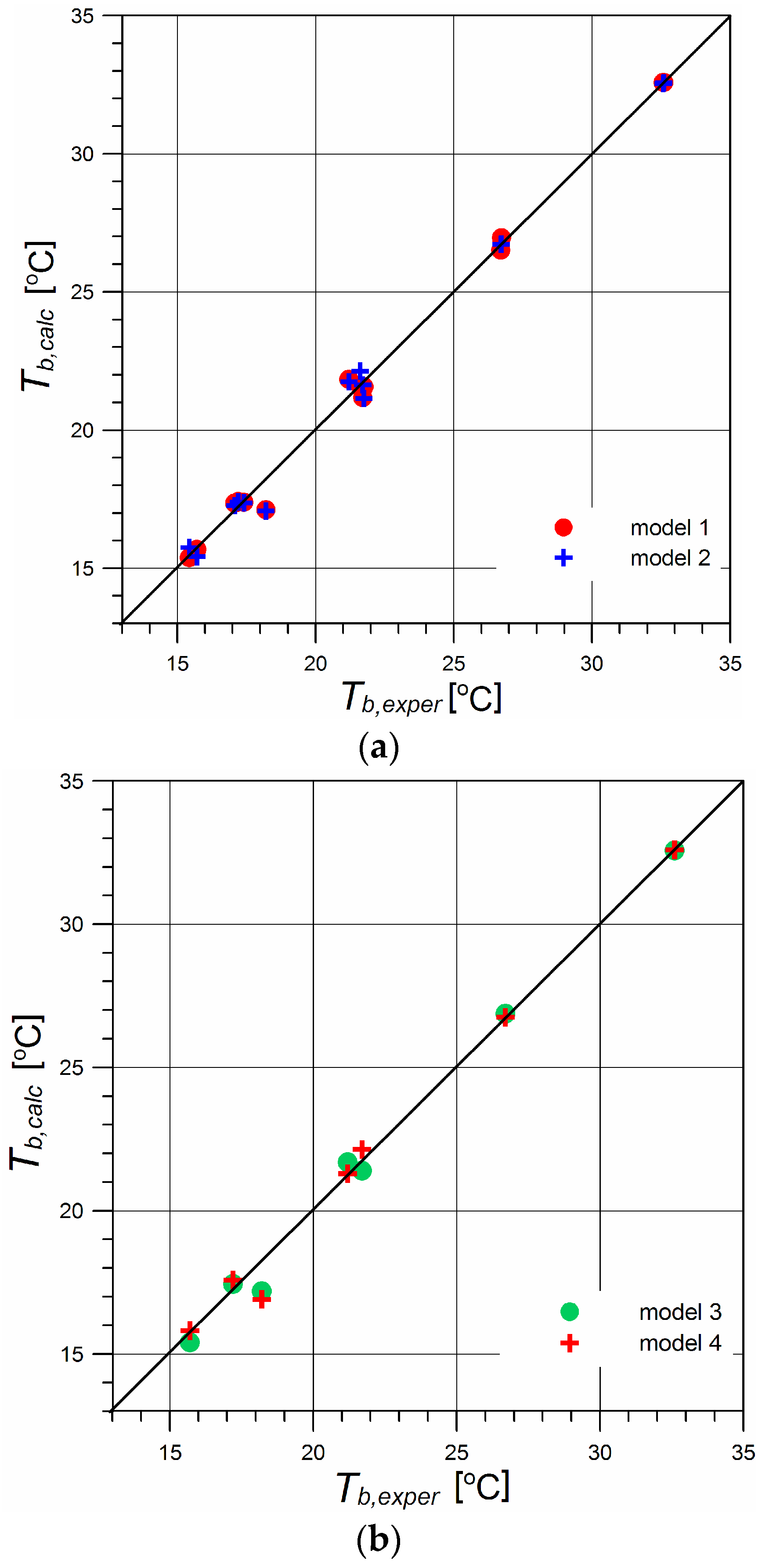
3. Empirical Dependencies

The T_b values may be determined using correlations developed on the basis of meteorological data, which has been proposed by Ouzzane et al. [4]. In their paper, the results of measurements collected from 15 locations with diversified climates are reported. The numerical values constituting the base for the development of the correlations were the T_b values (the dependent variable) and the following yearly average climatic data: ambient temperature, horizontal solar radiation, wind velocity, and dew point temperature (converted into sky temperature using Formula (6)). A linear correlation between the T_b and the listed quantities exists. It should be emphasised that the so-obtained correlation is not based on physical principles, thus it is of a purely empirical character. The values of the regression coefficients at the individual variables indicate the direction of changes in the T_b value, which increases with an increasing ambient temperature and horizontal solar radiation, and it decreases with increasing wind velocity. In the same paper [4], a second empirical correlation with a simplified character is also shown, which takes into account only one independent variable: ambient temperature.

In this paper an attempt to use the data gathered in paper [4] to develop a correlation based on an integrated form of the heat balance equation for the surface of the ground is made. Therefore, the effect of the moisture stream evaporated from the surface of the ground was also taken into account. It was assumed that the yearly average value of this flux is proportional to the yearly amount of precipitation per unit of the surface of the ground $\langle P\rangle$ [29]. Thus, the considered model has the following form:

$$\langle S\rangle -\epsilon \cdot \langle LW\rangle -\gamma \langle EV\rangle =h\cdot \Delta T$$

(26)

with substituted $\Delta T=T_b-\langle T_a\rangle$. Assuming that the evaporated moisture flux is equivalent to the heat flux needed to evaporate the water originating from the precipitation, the following is obtained [30]:

$$\langle EV\rangle =78\langle P\rangle$$

(27)

where $\langle EV\rangle$ [W/m²], $\langle P\rangle$ [m³/(m²year)].

The numerical values of the variables used in the developed equations are shown in

Table 2. Data for the correlations being developed.

		Elazig, Turkey	Oklahoma City, OK, USA	Shanghai, China	Hamah, Syria	Kiln, MS, USA	Brownsville, TX, USA	Dhahran, Saudi Arabia
Yearly average ambient temperature $\langle T_a\rangle$, °C [4]		13.0 *	14.8	15.6	18.1	19.6	22.7	27.4
Undisturbed ground temperature Tb, °C [4]		15.7	17.2	18.2	21.2	21.7	26.7	32.6
Yearly average dew point temperature $\langle T_{dp}\rangle$, °C [4]		1.78	7.94	11.66	6.71	14.24	17.61	14.99
Yearly av. effective sky temperature $\langle T_{sky}\rangle$, °C, Equation (7)		11.20	−4.29	−1.25	−1.94	4.19	9.43	12.09
Yearly av. long wave radiation flux $\langle LW\rangle$, W/m2, Equation (8)		120	106	98	119	93	97	120
Yearly total precipitation $\langle P\rangle$ m3/(m2year) [30]		0.577	0.829	1.134	0.441	1.594	0.690	0.088
Yearly av. evaporative heat flux $\langle EV\rangle$, W/m2, Equation (27)		45	65	88	34	124	54	7
Yearly av. solar radiation flux absorbed by the ground $\langle S\rangle$ [30]	kWh/(m2year)	1519	1606	1411	1763	1619	1890	2036
	W/m2	173	183	161	201	185	216	232
Yearly av. horizontal solar radiation $\langle S*\rangle$, W/m2 [4]		250.0	235.9	198.4	253.6	230.8	248.0	291.7

* Esen [31].

. Some of these data come from [4]; the data reported in [30] were also used. For the reasons described below, only the data corresponding to the conditions of a warm climate are shown.

The general form of the correlation is as follows:

$$\frac{\Delta T}{\langle EV\rangle }=b_0+b_1{X}_1+b_2{X}_2$$

(28)

Four detailed forms of the models were developed. All of them are based on the balance Equation (26).

Model 1.

The simplest model is based on the formula with one independent variable (Y = b₀ + b₁X):

$$\frac{\Delta T}{\langle EV\rangle }=-\frac{\gamma }{h}+\frac{1}{h}\cdot \frac{\langle S\rangle -\epsilon \cdot \langle LW\rangle }{\langle EV\rangle }$$

(29)

ε = 0.9 and $\langle LW\rangle$ = 63 W/m² were assumed. h = 33.0 W/(m²K) and γ = 0.61 were obtained. The maximum correlation error amounts to 1.1 °C.

The other models are based on dependencies with two independent variables (Y = b₀ + b₁X₁ + b₂X₂).

Model 2.

In the second model, the flux density $\langle LW\rangle$ is considered an unknown:

$$\frac{\Delta T}{\langle EV\rangle }=-\frac{\gamma }{h}+\frac{1}{h}\cdot \frac{\langle S\rangle }{\langle EV\rangle }-\frac{\langle LW\rangle }{h}\cdot \frac{\epsilon }{\langle EV\rangle }$$

(30)

ε = 0.9 was assumed. h = 25.3 W/(m²K), γ = 0.28 and $\langle LW\rangle$ = 110 W/m² were obtained. The maximum correlation error amounts to −0.6°C. The consistency of models 1 and 2 with the measurement results is shown in Figure 4a.

Model 3.

The following dependence was considered:

$$\frac{\Delta T}{\langle EV\rangle }=-\frac{\gamma }{h}+\frac{1}{h}\cdot \frac{\langle S\rangle }{\langle EV\rangle }-\frac{\epsilon }{h}\cdot \frac{\langle LW\rangle }{\langle EV\rangle }$$

(31)

The $\langle LW\rangle$ quantity was determined using Formula (8). h = 29.3 W/(m²K), γ = 0.59 and ε = 0.63 were obtained. The maximum correlation error amounts to −0.5 °C.

Model 4.

In this case the values of horizontal solar radiation $\langle S^{*}\rangle$ were used. The $\langle LW\rangle$ quantity was determined using Formula (8). Moreover, ε = 0.9 was assumed. The considered equation has the following form:

$$\frac{\Delta T}{\langle EV\rangle }=-\frac{\gamma }{h}+\frac{\beta }{h}\cdot \frac{\langle S^{*}\rangle }{\langle EV\rangle }-\frac{1}{h}\cdot \frac{\epsilon \cdot \langle LW\rangle }{\langle EV\rangle }$$

(32)

h = 14.2 W/(m²K), γ = 0.20 and β = 0.63 were obtained. The maximum correlation error amounts to 1.3 °C. The consistency of models 3 and 4 with the measurement results is shown in Figure 4b.

A list of the values of the individual models is shown in

Table 3. Characteristics of the models.

Model	S* or S	LW	ε	X1 (Equation (28))	X2 (Equation (28))
1	$\langle S\rangle$	constant	constant	$\langle S\rangle$ − ε$\langle LW\rangle$)/$\langle EV\rangle$	−
2	$\langle S\rangle$	coefficient of correlation	constant	$\langle S\rangle$/$\langle EV\rangle$	ε/<EV>
3	$\langle S\rangle$	data	coefficient of correlation	$\langle S\rangle$/$\langle EV\rangle$	$\langle LW\rangle$/$\langle EV\rangle$
4	$\langle S^{*}\rangle$	data	constant	$\langle S^{*}\rangle$/$\langle EV\rangle$	ε$\langle LW\rangle$/$\langle EV\rangle$

.

A list of the obtained dependencies is shown below:

$$T_b=\langle T_a\rangle +0.0303\langle S\rangle -0.0186\langle EV\rangle -1.72$$

(29a)

$$T_b=\langle T_a\rangle +0.0395\langle S\rangle -0.0109\langle EV\rangle -3.92$$

(30a)

$$T_b=\langle T_a\rangle +0.0341\langle S\rangle -0.0202\langle EV\rangle -0.0216\langle LW\rangle$$

(31a)

$$T_b=\langle T_a\rangle +0.0442\langle S^{*}\rangle -0.0143\langle EV\rangle -0.0633\langle LW\rangle$$

(32a)

The qualitative consistency of all the models is good: the values of the ΔT difference increase with increasing solar radiation and decrease with increasing amounts of precipitation and intensity of long-wave radiation. In all of the cases, reasonable values of the model coefficients were obtained: the values of the convection heat transfer coefficients are in the range of 14.2 to 33 W/(m²K), while the obtained values of the γ coefficient mean that from 20 to 64% of water originating from precipitation is evaporated from the surface of the ground.

A comparison of the model and the experimental results is shown in Figure 4a,b. As can be seen, the consistency is very good. However, the results presented pertain to warm climate conditions only. While processing the results for various climates, significant discrepancies occur. For T_b < 15 °C, the calculated T_b values are underrated in relation to the actual values. This discrepancy probably results from the fact that the general model does not take into account the periodical occurrence of snow cover on the surface of the ground, and this cover affects the values of the discussed heat fluxes significantly.

4. Conclusions

Both transfer of heat and mass occur on the surface of the ground. The heat necessary to evaporate water is extracted from the ground, lowering the temperature of the ground’s surface, affecting in turn the water vapour saturation pressure, the driving force of the mass transfer, and the moisture flux. Formula (25) was proposed for the calculation of the heat flux lost through the ground as a result of moisture evaporation. The formula is based on the non-linear form of the dependence of the saturated vapour pressure on temperature.

It results from the balance equation of the yearly average heat fluxes occurring on the surface of the ground that the calculated value of the difference between the T_b and the average ambient temperature is inversely proportional to the convection heat transfer coefficient h between the surface of the ground and the environment. Therefore, the possible accuracy of determination of the T_b value based on the heat balance equation strongly depends on the accuracy of the determination of the h coefficient.

The T_b value may be determined using the correlation Equations (29a)–(32a). These dependencies have a semi-empirical character and they are based on the thermal balance equation on the surface of the ground. The presented correlation equations take into account the heat flux for the moisture evaporation by relating the value of this flux to the yearly amount of precipitation. The presented correlation equations pertain to warm climate conditions.

References

1. Li, Y.; Geng, S.; Han, X.; Zhang, H.; Peng, F. Performance evaluation of borehole heat exchanger in multilayered subsurface. Sustainability 2017, 9, 356. [Google Scholar] [CrossRef]
2. Al-Khoury, R. Computational Modeling of Shallow Geothermal Systems; CRC Press: Boca Raton, FL, USA, 2012; p. 5. [Google Scholar]
3. Eskilson, P. Thermal Analysis of Heat Extraction Boreholes. Ph.D. Thesis, Department of Mathematical Physics, University of Lund, Lund, Sweden, 1987. [Google Scholar]
4. Ouzzane, M.; Eslami-Nejad, P.; Badache, M.; Aidoun, Z. New correlations for the prediction of the undisturbed ground temperature. Geothermics 2015, 53, 379–384. [Google Scholar] [CrossRef]
5. Kurevija, T.; Vulin, D.; Krapec, V. Influence of undisturbed ground temperature and geothermal gradient on the sizing of borehole heat exchangers. In Proceedings of the World Renewable Energy Congress, Linkoping, Sweden, 8–13 May 2011; pp. 1360–1367. Available online: http://www.ep.liu.se/ecp/057/vol5/017/ecp57vol5_017.pdf (accessed on 23 May 2017).
6. Gehlin, S.E.A.; Nordell, B. Determining Undisturbed Ground Temperature for Thermal Response Test. In ASHRAE Transactions: Research. 2003, pp. 151–156. Available online: https://www.diva-portal.org/smash/get/diva2:1014062/FULLTEXT01.pdf (accessed on 23 May 2017).
7. Yu, X.; Zhang, Y.; Deng, N.; Ma, H.; Dong, S. Thermal response test for ground source heat pump based on constant temperature and heat-flux methods. Appl. Therm. Eng. 2016, 93, 678–682. [Google Scholar] [CrossRef]
8. Zhou, S.; Cui, W.; Tao, J.; Peng, Q. Study of ground temperature response of multilayer stratums under operation of ground-source heat pump. Appl. Therm. Eng. 2016, 101, 173–182. [Google Scholar] [CrossRef]
9. Kusuda, T.; Achenbach, P.R. Earth Temperature and Thermal Diffusivity at Selected Stations in the United States; National Bureau of Standards Report Nr 8972. 1965. Available online: http://www.dtic.mil/dtic/tr/fulltext/u2/472916.pdf (accessed on 23 May 2017).
10. Popiel, C.O.; Wojtkowiak, J. Temperature distributions of ground in the urban region of Poznan City. Exp. Therm. Fluid Sci. 2013, 51, 135–148. [Google Scholar] [CrossRef]
11. Ouzzane, M.; Eslami-Nejad, P.; Aidoun, Z.; Lamarche, L. Analysis of the convective heat exchange effect on the undisturbed ground temperature. Sol. Energy 2014, 108, 340–347. [Google Scholar] [CrossRef]
12. Badache, M.; Eslami-Nejad, P.; Ouzzane, M.; Aidoun, Z. A new modeling approach for improved ground temperature profile determination. Renew. Energy 2016, 85, 436–444. [Google Scholar] [CrossRef]
13. Krarti, M.; Lopez-Alonzo, C.; Claridge, D.E.; Kreider, J.F. Analytical model to predict annual soil surface temperature variation. J. Sol. Energy Eng. 1995, 117, 91–99. [Google Scholar] [CrossRef]
14. Mihalakakou, G.; Santamouris, M.; Lewis, J.O.; Asimakopoulos, D.N. On the application of the energy balance equation to predict ground temperature profiles. Sol. Energy 1997, 60, 181–190. [Google Scholar] [CrossRef]
15. Herb, W.R.; Janke, B.; Mohseni, O.; Stefan, H.G. Ground surface temperature simulation for different land covers. J. Hydrol. 2008, 356, 327–343. [Google Scholar] [CrossRef]
16. Nam, Y.; Ooka, R.; Hwang, S. Development of a numerical model to predict heat exchange rates for a ground-source heat pump system. Energy Build. 2008, 40, 2133–2140. [Google Scholar] [CrossRef]
17. De Jesus Freire, A.; Alexandre, J.L.C.; Silva, V.B.; Couto, N.D.; Rouboa, A. Compact buried pipes system analysis for indoor air conditioning. Appl. Therm. Eng. 2013, 51, 1124–1134. [Google Scholar] [CrossRef]
18. Bortoloni, M.; Bottarelli, M.; Su, Y. A study on the effect of ground surface boundary conditions in modelling shallow ground heat exchangers. Appl. Therm. Eng. 2017, 111, 1371–1377. [Google Scholar] [CrossRef]
19. Fujii, H.; Nishi, K.; Komaniwa, Y.; Chou, N. Numerical modeling of slinky-coil horizontal ground heat exchangers. Geothermics 2012, 41, 55–62. [Google Scholar] [CrossRef]
20. Fujii, H.; Yamasaki, S.; Maehara, T.; Ishikami, T.; Chou, N. Numerical simulation and sensitivity study of double-layer Slinky-coil horizontal ground heat exchangers. Geothermics 2013, 47, 61–68. [Google Scholar] [CrossRef]
21. Demir, H.; Koyun, A.; Temir, G. Heat transfer of horizontal parallel pipe ground heat exchanger and experimental verification. Appl. Therm. Eng. 2009, 29, 224–233. [Google Scholar] [CrossRef]
22. Duffie, J.A.; Beckman, W.A. Solar Engineering of Thermal Processes; Wiley Inc.: New York, NY, USA, 2006; p. 149. [Google Scholar]
23. Klein, S.A.; Duffie, J.A.; Mitchell, J.C.; Kummer, J.P.; Thornton, J.W.; Bradley, D.E.; Arias, D.A. TRNSYS 17. A Transient System Simulation Program. Volume 4. Mathematical Reference; Solar Energy Laboratory, University of Wisconsin: Madison, WI, USA, 2017. [Google Scholar]
24. Khatry, A.K.; Sodha, M.S.; Malik, M.A.S. Periodic variation of ground temperature with depth. Sol. Energy 1978, 20, 425–427. [Google Scholar] [CrossRef]
25. Kupiec, K.; Larwa, B.; Gwadera, M.; Komorowicz, T. Modelling of heat transfer in the ground. Przem. Chem. 2016, 95, 1997–2002. [Google Scholar] [CrossRef]
26. Cengel, Y.; Ghajar, A. Heat and Mass Transfer: Fundamentals and Applications; McGraw-Hill: New York, NY, USA, 2010; p. 836. [Google Scholar]
27. Green, D.W.; Perry, R.H. Perry’s Chemical Engineers’ Handbook, 8th ed.; McGraw-Hill: New York, NY, USA, 2008. [Google Scholar]
28. McAdams, W.H. Heat Transmission; McGraw-Hill: New York, NY, USA, 1954. [Google Scholar]
29. Kiehl, J.T.; Trenberth, K.E. Earth’s Annual Global Mean Energy Budget. Bull. Am. Meteorol. Soc. 1997, 78, 197–208. [Google Scholar] [CrossRef]
30. Gaisma. Sunrise, Sunset, Dawn and Dusk Time around the World. Available online: www.gaisma.com (accessed on 23 May 2017).
31. Esen, H.; Inalli, M.; Esen, M. Numerical and experimental analysis of a horizontal ground-coupled heat pump system. Build. Environ. 2007, 42, 1126–1134. [Google Scholar] [CrossRef]
32. Carslaw, H.S.; Jaeger, J.C. Conduction of Heat in Solids, 2nd ed.; Clarendon Press: Oxford, UK, 1959; pp. 64–70. [Google Scholar]
Figure 1. Heat fluxes on the surface of the ground.
Sustainability 09 02055 g001
Figure 2. Influence of the evaporation rate parameter f and the relative humidity of air (RH) on Tb.
Sustainability 09 02055 g002
Figure 3. Influence of the convection heat transfer coefficient h and the S on Tb.
Sustainability 09 02055 g003
Figure 4. Comparison of accordance of the correlations: (a) model 1 and 2, (b) model 3 and 4.
Sustainability 09 02055 g004