Short-Term Multiple Forecasting of Electric Energy Loads for Sustainable Demand Planning in Smart Grids for Smart Homes

Abstract

Energy consumption in the form of fuel or electricity is ubiquitous globally. Among energy types, electricity is crucial to human life in terms of cooking, warming and cooling of shelters, powering of electronic devices as well as commercial and industrial operations. Users of electronic devices sometimes consume fluctuating amounts of electricity generated from smart-grid infrastructure owned by the government or private investors. However, frequent imbalance is noticed between the demand and supply of electricity, hence effective planning is required to facilitate its distribution among consumers. Such effective planning is stimulated by the need to predict future consumption within a short period. Although several interesting classical techniques have been used for such predictions, they still require improvement for the purpose of reducing significant predictive errors when used for short-term load forecasting. This research develops a near-zero cooperative probabilistic scenario analysis and decision tree (PSA-DT) model to address the lacuna of enormous predictive error faced by the state-of-the-art models. The PSA-DT is based on a probabilistic technique in view of the uncertain nature of electricity consumption, complemented by a DT to reinforce the collaboration of the two techniques. Based on detailed experimental analytics on residential, commercial and industrial data loads, the PSA-DT model outperforms the state-of-the-art models in terms of accuracy to a near-zero error rate. This implies that its deployment for electricity demand planning will be of great benefit to various smart-grid operators and homes.

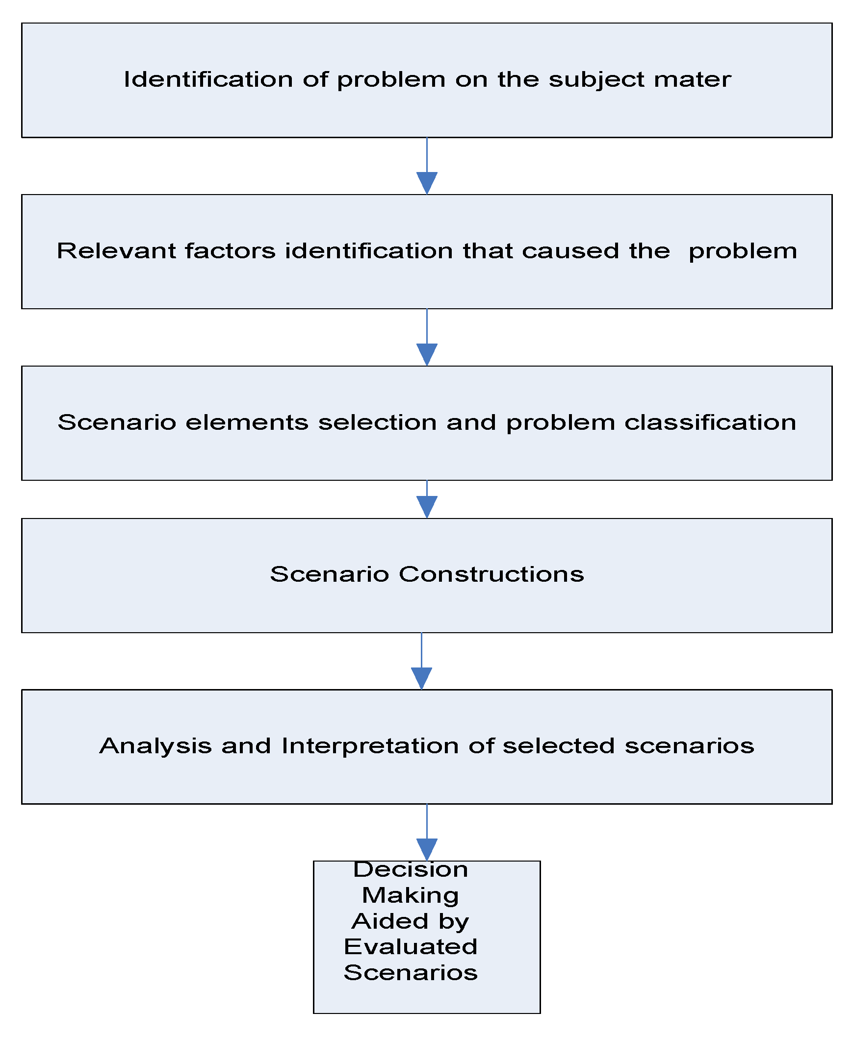
1. Introduction

Predicting electricity demand is crucial, since it plays a significant role in the administration, decision-making and demand planning of utility power supply operations [1]. Effectiveness and accuracy in terms of extremely reduced forecasting error of a predictive model cannot be overemphasised, as load forecasting guides power grid operations and power station construction planning. Forecasting is also important for the sustainable development of the electric power industry [2]. Short-term load forecasting (STLF), the generic abbreviation for a model that can predict future load consumption with a lead time of up to a few hours or a few days, has been undergoing constant improvement in the last few decades [3]. Inaccurate load forecasting for effective demand planning remains a difficult and critical challenge [4]. This problem invariably increases the operating costs of electricity suppliers [5]. Thus, there is need for improved STLF in terms of potential error reduction, which could improve the reliability and efficiency of power generation [6]. Figure 1 is an example of the percentage differences between the actual load and forecast load consumption, used by different classes of consumers from different locations in Australia. The Negative (−ve) bars and points shown above the x-axis in Figure 1a–c mean the load forecasting values were low compared to the actual consumption after calculating their differences. In addition, the positive (+ve) bars and points shown below the x-axis in Figure 1a–c depict the forecasting values were high in relation to the actual electricity consumption after their computation differences.

In addition to the forecasting problem relating to disparity between electricity demand and forecast, Figure 1c reveals the extensive differences between the actual and the forecast load. The positive section in the trend chart depicts that the utility has over-predicted the future load and the negative section indicates that the utility has under-predicted the future load consumption.

Classical models have been used but have proven inefficient in short-term load forecasting in a smart grid (SG) [9]. In statistical modelling techniques, regression and time-series models were a huge success, and, more recently, computationally intelligent techniques such as artificial neural networks (ANNs), support vector machines (SVMs), self-organisation maps (SOMs), and fuzzy logic have contributed immensely to STLF implementation. These models are excellent and have been applied in electricity prediction; however, because of uncertainty in the nature of electricity consumption, they still require improvement with regard to accuracy when used for short-term load forecasting [3]. However, cooperative short-term load techniques, which involve collaboration of more than one model, have proven to be more efficient and accurate [10]. In this regard, cooperative models can drastically reduce the large forecasting errors inherent in the classical techniques [1].

Research Question and Outline

This paper considers the development of a near-zero error cooperative model, integrating probabilistic scenario analysis and a decision tree (PSA-DT) technique, and poses the question “How can an efficient cooperative model be developed for STLF of electric energy loads in smart grids for smart homes?” The model uses a probabilistic method to obtain the initial predictive load consumption with a high level of confidence. Prior to making the final accurate decision for productive planning, a DT model is integrated with the probabilistic model. The major contributions of this paper are as follows:

• Development of a cooperative PSA-DT model, integrating the concept of probabilistic scenario analysis and decision tree techniques for short-term load forecasting and sustainable economic planning of electricity demand in an SG.
• Detailed experimental evaluations of the PSA-DT and its benchmarking with many state-of-the-art models, using publicly available data from [11,12] in terms of near-zero forecasting errors in the predictive paradigms for smart homes.

To the best of the knowledge of the authors, this research produces a low predictive error rate compared to other classical models described in Section 2.2. Notably, the remaining parts of this paper are arranged in the following order: Section 2 provides a detailed introduction to an SG, framework and data collection process within the grid. In the same section, a review of the existing state-of-the-art model will be discussed. In Section 3, the suggested PSA-DT model is presented, with a detailed explanation, in conjunction with evaluation techniques. In addition, the underlying mathematical analysis in the model will be discussed. Section 4 discusses the various experiments and evaluation of the model, and concluding remarks are shared in Section 5.

2. Preliminaries

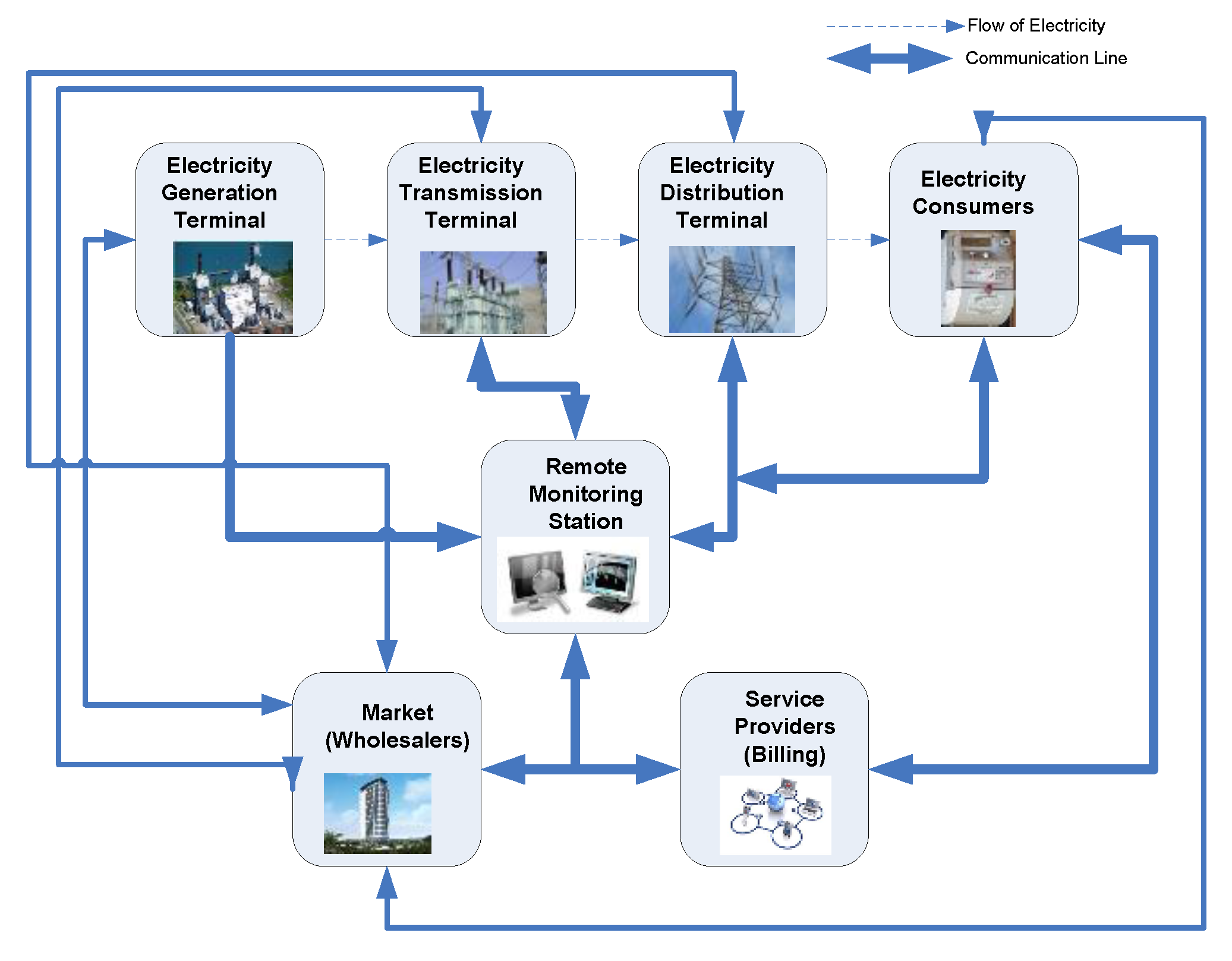
2.1. Smart-Grid Metering

Information and communication technology (ICT) is one of the essential components of technology-driven industries in today’s economy and its uses in renewable energy are no exception. ICT has been integrated into renewable energy, especially the power grid, in order to make such grids more intelligent, and this development is popularly referred to as SG. SG is one of the most critical components in a classical power grid containing several smart objects such as smart meters, smart devices, sensors, actuators and communication infrastructure for seamless communication among the SG components. SGs can be referred to as intelligent power grids (IPG). An IPG forms its chain from the energy generation point through power transmitting infrastructure and distribution networks to smart homes (final electricity consumer), such as houses, factories, public lighting, smart appliances and electric vehicle charging infrastructure, as shown in Figure 2, which captures the SG conceptual model. In addition, making such a power grid an intelligent one requires some level of ICT involvement such as hardware, software and firmware aimed at ensuring proper control and remote monitoring of the grid and maintaining a real-time balance between electricity generation and consumption. Moreover, electricity consumers drive the production from the power grid, and it is necessary to have foreknowledge of its future demand owing to population expansion.

Forecasting the future consumption of electricity within an SG is an essential aspect of power system planning and operation of SG systems. In every utility, load forecasting forms the key yardstick for pricing the required load generation for consumers. Electricity load forecasting, being the focus, can be a short-term, middle-term or long-term load. These differences depend solely on the requisite forecasting period, i.e., short-term forecasting focuses on one-hour to one-week future prediction, the medium term corresponds to one-week to one-year future prediction, while long-term forecasting focuses on more than a year in advance [6]. The focus of this research is short-term load forecasting and the data being used for the future prediction are hourly and 15-min interval data obtained from components of an SG, being the result of electricity consumption at different times of the year. Different residential properties, commercial offices and industrial sectors form the consumer section of an SG, as shown in Figure 2. Furthermore, various sensors, such as temperature and pressure sensors and other data collection devices, are installed on customers’ premises to aid data collection before transmitting it to a central repository for further analysis. It is noteworthy that in a twenty-first century electrical power grid infrastructure, the aims are to improve efficiency, security and reliability via intelligent control, power converters, ICT (hardware and software), sensing and metering and effective energy management techniques based on electricity demand optimization and network availability.

Prior to any prediction of the future load, it is essential to visualise the trends of the historical electricity load consumption, as shown in Figure 3, Figure 4 and Figure 5. The various figures depict the load consumption over time. This trend helps to see the various patterns of consumption within the residential, commercial and industrial sectors from the collected data.

From the virtualisations in Figure 4 and Figure 5, one can see different patterns of electricity consumption from the classes of data. The figures show diverging low, medium and high load consumptions for residential, commercial and industrial users. The consumption disparity depicts how loads are consumed by different groups at different times, and this helps most utilities determine load behaviour on a class-by-class consumer basis.

2.2. Forecasting Modelling Techniques for Energy Load

STLF within an SG can be effectively addressed from two major approaches, using either artificial intelligence (AI) techniques or statistical methods. Some of the reviews given in [13] for electric load forecasting range from time-series to regression-based methods, being statistically based techniques. Artificial intelligence methods, ranging from ANN, fuzzy inference techniques and SVMs, to particle swamp optimisation and genetic algorithms, are mostly used for optimization.

Table 1. Comparison of Load Forecasting Methods.

Energy Load Forecasting Techniques	Specific Model Used	Strength	Weakness	Error Rate with Respect to the Data Used
Regression [19,20]	Linear Regression and Multiple Linear Regression	Very useful in non-real time forecasting. Functional relationship between previous, forecast load and other factors such as weather, time of the day.	Not accurate for real time load and unable to handle nonlinear load consumption. Adding parameters make it unstable.	4.665% 21.87%
Time-series Analysis [20,21,22]	Auto Regressive Moving Average, Auto Regressive Integrated Moving Average, Deterministic decomposition.	They possess abilities to accommodate seasonal component effects.	They suffer numerical instability	1.48–1.99%
Artificial Neural Network [23,24]	Multilayer Perceptrons, Back Propagation Algorithm, Steepest descent Error Back Propagation.	Ability to handle nonlinear relationships in load consumption by adjusting its weight during the training process.	Large amounts of data are needed to train the model and complexity in the training of such data.	2.9% 6.609%
Fuzzy Inference System [19,25]	Defuzzification Method using Centre of Area, Middle of Maxima, Last of Maxima and Centre of gravity	Faster and more accurate in performance including simplicity in rule formation.	Selection of membership function to form its rule is based on trial and error.	2.58%, 5.831% and 1.794%, 9.53%
Support Vector Machine [15,26]	Support Vector Regression using Incremental Learning Algorithm Support Vector Regression	It enhances higher feature space dimensionality by using ε-insensitive loss for linear regression computation and reduction in model complexity.	Choosing of suitable kernel and difficulties in its interpretation are major concerns	4.2306% 1.57–4.28% 1.95–3.48

shows a brief comparison of some of the most widely used STLF techniques in terms of their strength, drawbacks and possible predictive error obtained from the literature.

2.2.1. Regression-Based Method

This model is a widely used statistical technique for electric load forecasting [14]. It is used for modelling the relationship between load consumption and other factors such as weather and day type, and it tends to measure the extent of the relationship between the dependent and independent variables [15]. It has been most relevant in offline (non-real time) forecasting, since it is generally unstable for online forecasting because it requires many external variables that are difficult to introduce into an online algorithm [14].

2.2.2. Time Series Analysis Method

This involves time series plots and extrapolating such patterns using a set of previously collected data to predict the future load [15]. The approach has gained popularity in online forecasting by making it possible to accommodate some weather information [16] and this has improved the accuracy level and ease of online implementation. Non-availability of weather parameters limits the efficiency of this technique and causes some weaknesses in the predictive abilities using this technique [15].

2.2.3. Exponential Smoothing Method

The success of this method can be traced to both online and offline forecasting. Its simplicity and cost make it an appealing forecasting tool [16]. However, it has poor long-range accuracy with regard to weather information. Therefore, this technique cannot account for weather-related load changes.

2.2.4. Expert System Approach

Being a rule-based technique resulting from the improvement in the AI domain, the expert system approach has a retractable reasoning instinct with adjustable cognitive abilities with new information [15]. It uses an “if-then” rule base for its inference; therefore, such rules require constant updates for effective performance.

2.2.5. Artificial Neural Network-Based Techniques

This is an unsupervised machine-learning method that involves inter-connection of numerous neurons, which can be used to accurately learn the characteristics of non-linear relationships of input and output pairs of data. This is one of the major merits of the model compared to other statistical approaches [17]. In addition, Hahn et al. [18] found that several neural networks performed best with a small mean percentage error between 2.35% and 2.65%, and lesser spreading of the errors. However, neural networks require significant training to understand the model [17].

2.2.6. Support Vector Machine (SVM)

A SVM is very powerful, especially for solving classification and regression issues [15]. SVM is used for non-linear mapping of datasets into prominent dimensional features via kernel functions, a class of pattern analysis algorithm that performs better than the statistical techniques. Chen et al. [19] discovered that support vector regression avoids under-fitting and over-fitting as well as regularisation. However, choosing of a suitable kernel during the analytical phases and difficulties in its interpretation are major concerns in this technique [15].

Despite the classical methods in Table 1, there have been good testimonies about cooperative methods compared to classical methods in terms of performance [10,27].

2.3. Theoretical Techniques

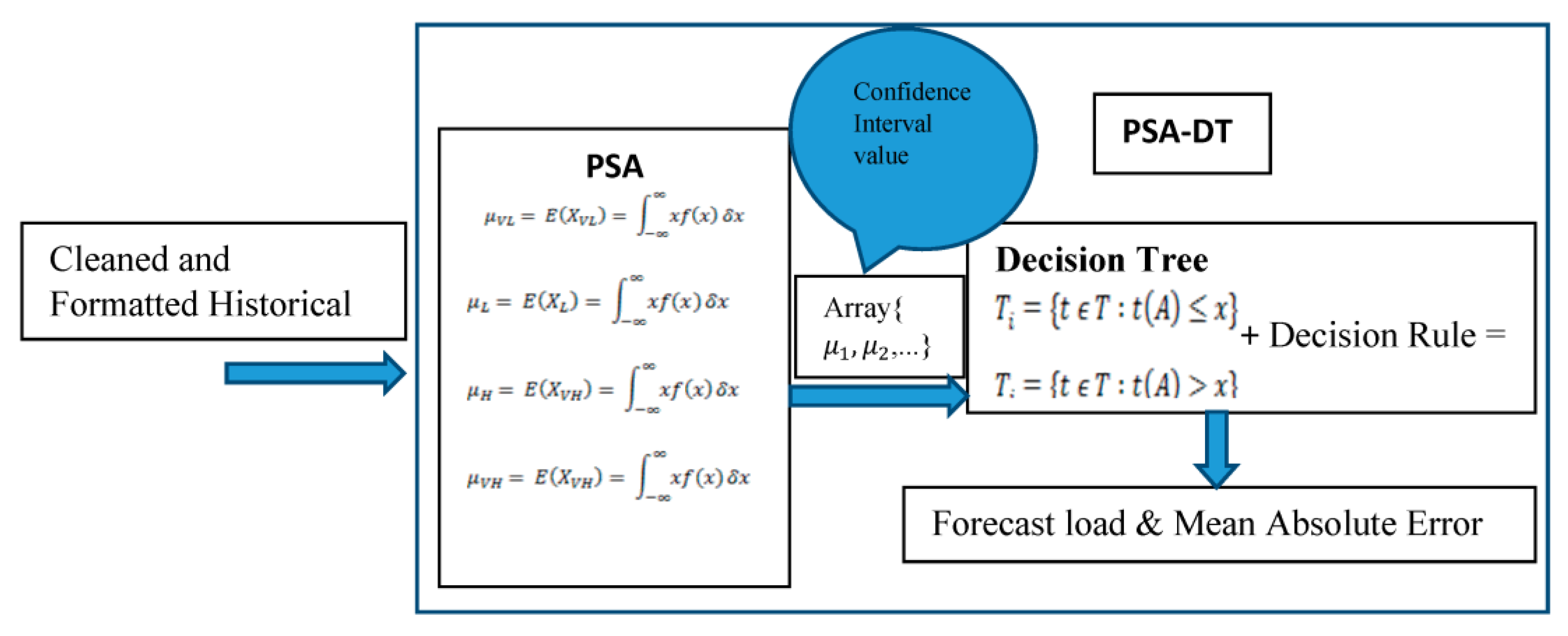
2.3.1. Probabilistic Scenario Analysis (PSA)

PSA, being the use of a probabilistic model over various scenarios, foresees and evaluates various possible occurrences of an event in the future [28,29]. It is mostly used in the financial world to make extensive projections into the future. Considering the technique and its vast usage in management for future forecasting, several researchers have come up with diverse processes in performing good scenario analysis [30], which can easily be combined with the probability model [31] to generate a sampled expected outcome based on randomly generated events [32]. In summary, the scenario process depicted below in Figure 6 will aid any activity considering scenario analysis as a method of future prediction. In conjunction with the probabilistic theory, the expected mean, deviation from mean and the degree of confidence of accepting the mean are essential statistical tools meant to be used for each scenario. Because of the continuous nature of electricity consumption, the expected mean will be computed as a random variable X between two load points shown in Equation (1), where $f\left(x\right)$ is a probability density function between two loads, a and b.

In the proposed technique, especially during simulation processes, the cumulative probability f(x) of the load is being computed as a non-decreasing function with probability values between 0 and 1. In this regard, the expected mean in Equation (1) generated during this random process will have a certain level of confidence, which falls between the confidence interval for the entire load samples usually known as the t-interval, as shown in Equation (2).

$$mean\left(\mu \right)=E\left(X\right)={{\displaystyle \int }}_{-\infty }^{\infty }xf\left(x\right)\delta x\mathrm{where}f\left(x\right)=P\left(a\le x\le b\right)$$

(1)

$${\mathit{t}}_{\mathit{i}\mathit{n}\mathit{t}\mathit{e}\mathit{r}\mathit{v}\mathit{a}\mathit{l}}=x\pm T_{\raisebox{1ex}{$\alpha $}\!\left/ \!\raisebox{-1ex}{$2$}\right.,n-1}\times \frac{\sigma }{\sqrt{N}}$$

(2)

where E(X) $isa\mathit{p}\mathit{o}\mathit{i}\mathit{n}\mathit{t}\mathit{e}\mathit{s}\mathit{t}\mathit{i}\mathit{m}\mathit{a}\mathit{t}\mathit{e}of\mu$, $\frac{\sigma }{\sqrt{N}}=\mathit{s}\mathit{t}\mathit{a}\mathit{n}\mathit{d}\mathit{a}\mathit{r}\mathit{d}\mathit{e}\mathit{r}\mathit{r}\mathit{o}\mathit{r}\mathit{o}\mathit{f}\mathit{t}\mathit{h}\mathit{e}\mathit{m}\mathit{e}\mathit{a}\mathit{n}$ and $T_{\raisebox{1ex}{$\alpha $}\!\left/ \!\raisebox{-1ex}{$2$}\right.,n-1}$ × $\frac{\sigma }{\sqrt{N}}=\mathit{e}\mathit{r}\mathit{r}\mathit{o}\mathit{r}\mathit{m}\mathit{a}\mathit{r}\mathit{g}\mathit{i}\mathit{n}$.

2.3.2. Decision Tree (DT)

A DT uses a tree-like pattern to present various possibilities for its decision route and the result of each route in order to decide effectively on the path to take, depending on whether it is a classification or regression problem. Concepts such as entropy and information gain must be predetermined for an effective split in the classification problem, while standard deviation from the mean forms the major criterion for a split in the regression problem.

Entropy: This is a measure of disorderliness or impurities in the sample space. In every sample space, there are data that might not contribute to the decision made by the DT model; the model tries to make its decision by ensuring that the decision boundaries are void of impurities as much as possible. Entropy computation has been formalised by Shannon [32,33]. Let us assume a random variable X with values x_i and probability $Pr\left(x_i\right)$ has it entropy in Equation (3).

$$H\left(X\right)=-{\displaystyle \sum }_i\mathrm{Pr}\left(x_i\right)log2\mathrm{Pr}\left(x_i\right)$$

(3)

In addition, information gain, which is meant to be maximized in the decision processes, has the lowest value as zero (0) and the highest value as one (1). In some other texts, this is called gain ratio, which draws many of relationships from the entropy. It is mostly defined by the difference between the initial and the final entropy, as shown in Equation (4).

$$IG\left(X,i\right)=H\left(X\right)-H(X|i)$$

(4)

In general, let us define the training samples $T$ containing a time series load data $\left(x,y\right)=\left(x_1,x_2,x_3,x_4,\dots ..,x_n,y\right)$ where $x\in vals\left(i\right)$ is a value of the ith attribute of the sample x and y. The information gain for the ith attribute in terms of $H\left(T\right)$ entropy is given in Equation (5).

$$IG\left(T,i\right)=H\left(T\right)-{\displaystyle \sum }_{v\in val\left(i\right)}\frac{abs(\{x\in T|x_i=v\})}{abs\left(T\right)}.H(\{x\in T|x_i=v\})$$

(5)

Standard deviation (SD), otherwise called standard error (SE), describes the expected variations in the mean of a population and it can be written mathematically as presented in Equation (6).

$$SD=\sqrt{(\frac{1}{N-1}{\displaystyle \sum }_{i=1}^n{\left(Y{i}^{\prime }-Y\right)}^2)}$$

(6)

A DT can be built using Greedy top-down construction, which is the most widely used technique in tree growing [34]. It is structured in a top-down pattern considering all the data and then builds up various subsets of the tree, which is being managed in a recursive manner. Having constructed the tree, one has to deal with the problem of finding the right tree size, which can be managed via pruning [34].

Briefly, in Section 4, during the PSA-DT model evaluation, we use the DT regression function in scikit-learn that implemented these concepts, and we also improved the learning algorithm by making such a prediction more generalised and sensitive to new datasets through bias-variance trade-off.

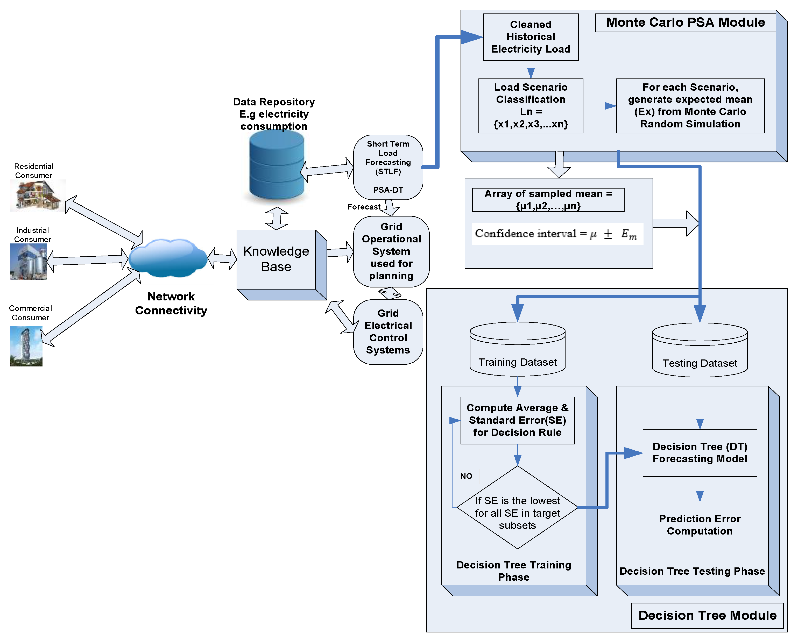
3. Development of Cooperative PSA-DT Model for Short-Term Load Forecasting

This section mainly focuses on the development of a cooperative model for short-term load forecasting in an SG environment. It uses the predictive result for effective future demand and operational planning. In this model, load consumption from various classes of consumers, such as residential, commercial and industrial was, considered, and the collected historical load data from different classes of consumers were cleaned and formatted for effective integration. The PSA-DT cooperatively functions as an interaction between scenario analysis with probabilistic focus and a DT model as shown in Figure 7. Probabilistic results of each scenario analysis form a list structure. In addition, the lists generated have some confidence value to show that the contents of the list have a high degree of confidence belief. This list is then passed to the DT to generate predictive value with low mean absolute error (MAE).

Considering some of the components in Figure 7, these were divided into the historical data repository, grid operational planning systems and the PSA-DT framework. The historical data were generated from various power sensors installed within the SG to record the different categories of users’ electricity consumption. Users such as residential, commercial and industrial producers generate a time-based load consumption, filtered via the knowledge-based system and stored in a repository for future predictions and research. The grid operational system comprises the control systems and the various operational components such as smart meters and several planning tools, among which is the STLF model for effective load planning. The PSA-DT framework details the process of using both Monte Carlo PSA and a DT for a near-zero short-term load predictive solution, as shown in Figure 7.

3.1. Confidence Interval and Degrees of Freedom

This is usually in range and defined as the probability value within which the value of a parameter falls. It is an indicator of how stable an estimate (E(X)) is and it measures how close the measurements are to the initial estimate in some repeated experiments. With the mean ($\mu )$ and standard deviation ($\sigma )$, the estimate at 90%, 95% or 99% confidence level can be computed before such an estimate of a high confidence degree and with uniform probability of occurrence can be fed into the DT for final prediction of future load consumption.

$$\mathrm{Confidence}\mathrm{interval}=\mu \pm E_m$$

(7)

Degree of Freedom: The degree of freedom (DF) is the number of independent items of information used for calculating an estimate. Usually, DF is one less than the sample size.

DF = Sample Size (N) − 1

(8)

3.2. PSA-DT: Monte Carlo Probabilistic SA Modelling

Because of uncertainty about future load consumption, the PSA model was based on Monte Carlo method. It involves the use of probabilistic simulation techniques to compute the future sampled demand of load consumption. This process uses both probability and scenario analysis. In the scenario section shown in Figure 8, PSA was built around the cleaned and formatted historical load $L=\left\{l_{1,}{l}_{2,},l_{3,},l_{4,}\dots ..l_{n,}\right\}$. The load was split into four major parts, namely very low (VL), low (L), high (H) and very high (VH), forming each scenario case. At every point in time, any load consumption (L_o) can be a member of any of the subsets of the entire load-set. For each subset, we then find the probability of each scenario to generate its expected value for each subset. The expected mean of each scenario was also obtained through various random experiments using Monte Carlo simulations. For each event generated in the random experiment, the mean was calculated repeatedly to generate another future mean during the subsequent random experiment. In the final set of mean loads, the confidence interval of mean, shown numerically in Section 3.6, is calculated and stored in conjunction with the mean in the array structure for further analysis with the DT model, as also shown in Figure 8.

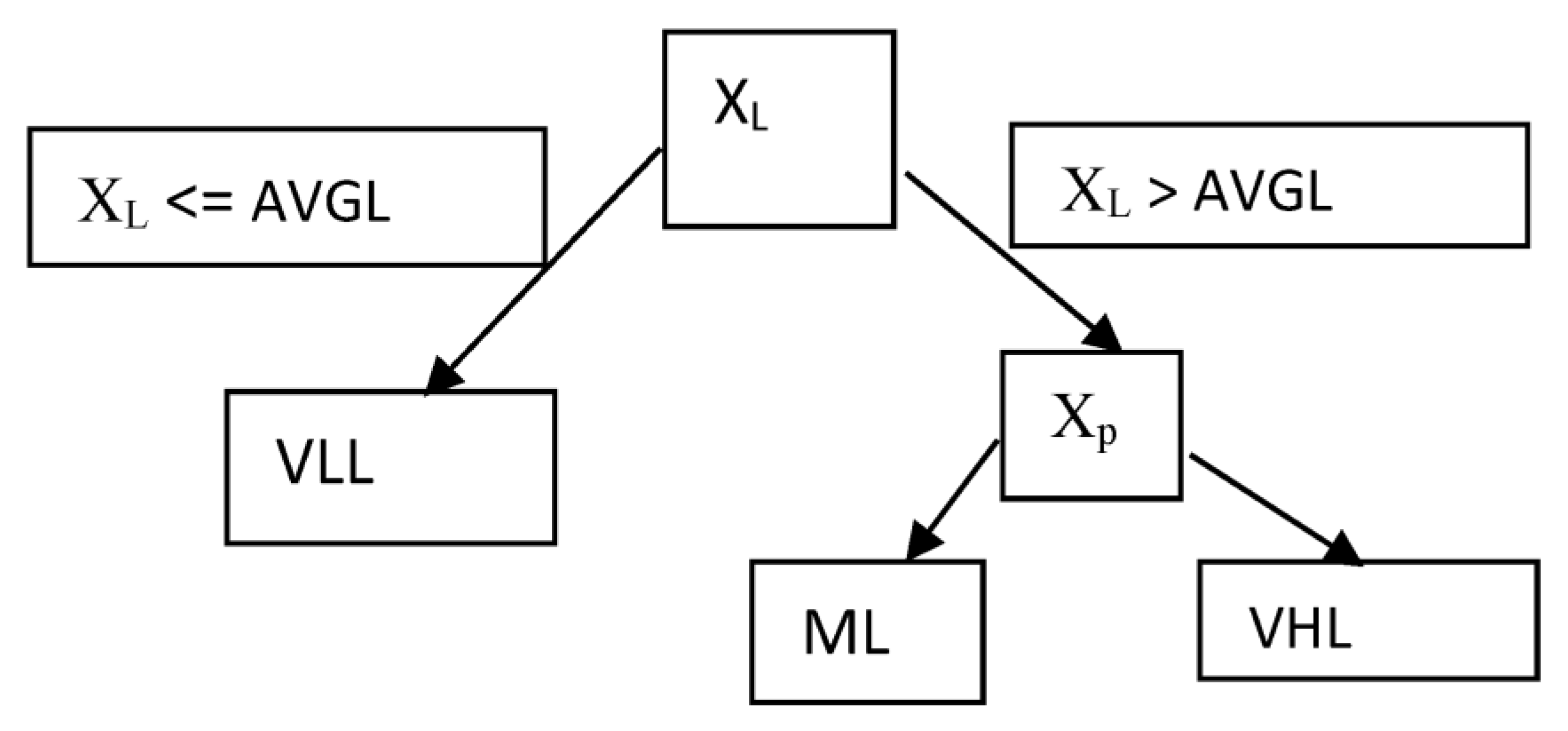
3.3. PSA-DT: Decision Tree Modelling

Using the DT model for final prediction of the short-term load requires the expected mean in the list generated from the Monte Carlo experiment to be divided into training and test data. In each of the features in the training set, a set average and the standard error for each of the training feature were calculated; a target variable within the training set with least standard error was selected to enhance the split point of the training set into two sets, namely S₁ and S₂. These operations were then carried out recursively until the leaf nodes were reached. In addition, the lowest error used in determining the split point shows how close the predicted value can effectively fit the test value with a near-zero error value. The prediction and the MAE for the load consumption were finally computed. Based on the DT section in the framework shown in Figure 8, the operations described above were broken down for quick view and comprehension for similar approaches, using the decision rule in Figure 9.

Definition: 

Consider a DT structure for the load recognition problem described by the following properties:

X_L is the load consumption, X_p is the absolute weather status and Y constitute a set of possible behaviour exhibited by the entities in X, which are {very low load (VLL), moderate load (ML), very high load (VHL)}.

In this case, Figure 9 now shows the model situation where Y depends on X after the average load (AVGL) has been computed.

Considering Figure 9, the tree has a root as X_L growing downwards to X_p and several leaf nodes, namely VLL, ML and VHL. This formation was based on the following decision rule:

• If X_L <= AVGL, Y = “VLL”.
• If X_L ∈ Z, where Z > AVGL and X_p = “average weather”, then Y = “ML”.
• If X₁ ∈ Z, where Z > AVGL and X_p = “hash weather”, then Y = ”VHL”.

The VLL, ML and VHL form the predicted load at every decision node such as X_L and X_p. As described in Section 2.3.2, these nodes were formed based on the computation of standard errors for each of the sample elements and selecting the least error in conjunction with the corresponding samples.

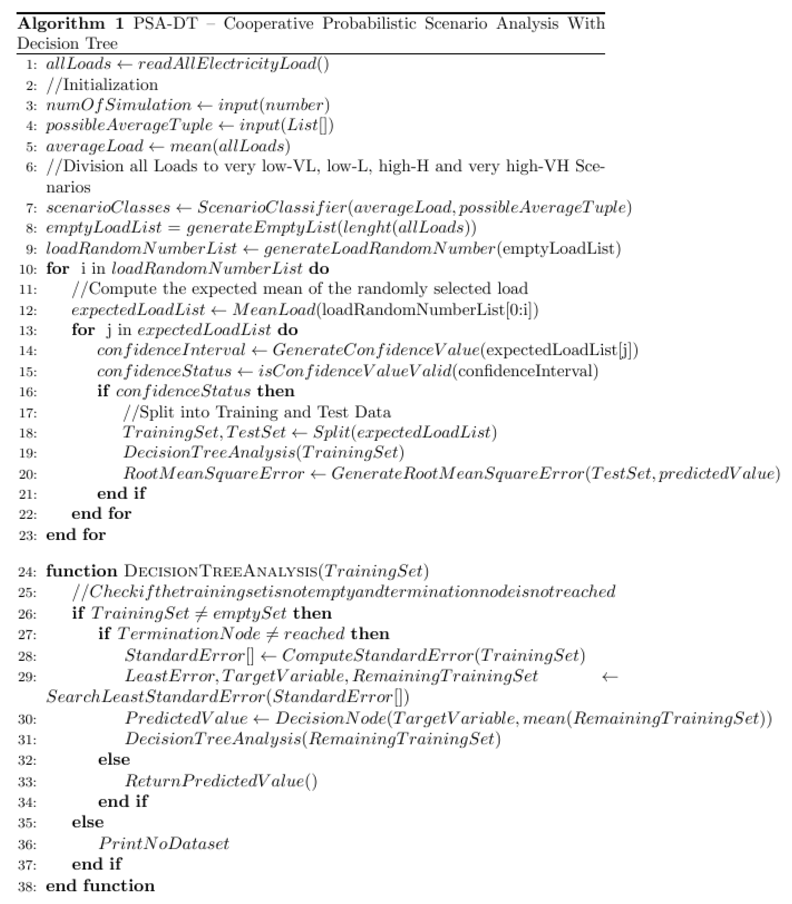
3.4. PSA-DT Algorithmic and Mathematical Analysis

Figure 10 is the pseudo-code used to develop implementation for the PSA-DT model. Having read all the electricity load data from the stored repository, the number of simulations for the experiment was inserted. An empty list was generated and the load was finally classified into different scenarios as discussed earlier. The random number of sampled mean was also computed in order to produce the expected mean being stored in an array. The resulting list was used to compute the confidence interval, as revealed in the pseudo-code in Figure 10.

3.5. Scoring and Evaluation Mechanisms

3.5.1. Cross-Validation Scheme

One of the major scoring and evaluation schemes is a cross-validation scheme, popularly known as K-fold cross-validation (K-fold CV). Its primary aim is to improve predictive performance in a statistical model. It is a systematic repetition of the training/testing procedure several times, which aims to lower the associated variance that dominates the single run of training/testing splitting techniques. When this method serves as an improvement mechanism, the entire dataset will be split into k equal sizes known as folds. A combination of k-1 folds will be used to train the model and testing will make use of the remaining one fold, but the fold for testing will be unique at every iteration of the k-fold space. In summary, the major aim of cross-validation is to avoid overfitting.

Implementing the cross-validation task, the following procedure is followed by each of the k-folds:

• Model training using k-1 of the folds as training data; and
• Validating the resulting model on the remaining set of data i.e., it is used as test data to compute its accuracy, which is a performance measurement.

The average of the computed value in loop therefore forms measured performance by k-fold cross-validation.

3.5.2. Mean Absolute Error

In addition, MAE is an evaluation metric for predictive modelling performance used to measure the level of closeness of the prediction to the actual outcome. It can be calculated via Equation (9),

$$MAE=\frac{1}{N}{{\displaystyle \sum }}_{i=1}^n\left|y_i-x_i\right|$$

(9)

where n is the number of observations, and $\left|y_i-x_i\right|$ is the absolute errors between the predicted and actual load.

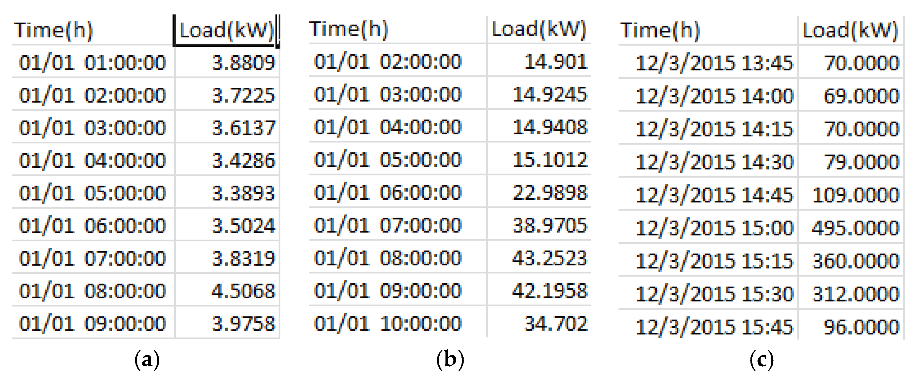
3.6. Numerical Scenario

(i) For Residential Load Consumption

Supposing there is a sample set of very high residential load consumption from an SG, $R{L}_{vh},$ which is equal to {3.8809, 3.7225, 3.6137, 3.4286, 3.3893, 3.5024, 3.8319, 3.74693021, 3.74657042, 3.74643688} in Kw/h. Based on the randomly generated estimated load data from Monte Carlo simulations through randomly sampled residential load from the set $R{L}_{vh}$, the following list, ${\mu }_{vh}$ = {3.74747941, 3.74715633, 3.74683391, 3.74706542, 3.74670404, 3.74693522, 3.74679607, 3.74693021, 3.74657042, 3.74643688} was generated as expected load in the simulated experiment with mean ($\mu$) equals 3.7499 and standard deviation ($\sigma$) equals 0.1224.

From Equation (7), the 95% confidence level, sometimes called the margin error ($E_m$), can be obtained from the calculation in this section.

Using Equation (2),

• N = sample size = 10
• $\mu =\mathbf{3.7499}and\sigma$ = Standard deviation = 0.1224
• $\alpha$ = Confidence Level = 95% = 0.95.
    From Equation (8) DF = 10 − 1 = 9
• $\frac{\sigma }{\sqrt{n}}$ = Standard Error = $\frac{\mathbf{0.1224}}{\sqrt{\mathbf{10}}}$ = 0.0387.

Being a component in Equation (2), $T_{\raisebox{1ex}{$\alpha $}\!\left/ \!\raisebox{-1ex}{$2$}\right.}$ = Confidence Coefficient = $T_{value}$ (1-confidence level)/2 = (1 − 0.95)/2 = 0.025.

We can then extract the result of $T_{value}$ (0.025) = 2.262 from T distribution section in [33] and also $E_m$ = 2.262 × 0.0387 = 0.0875

Therefore, the confidence interval at 95% confidence degree = 3.7499 ± 0.0875:

• lower limit with 95% confidence interval = 3.7499 − 0.0875 = 3.6624; and
• upper limit with 95% confidence interval = 3.7499 + 0.0875 = 3.8375.

Despite some low load consumption in $R{L}_{vh},$ such as 3.4286 Kw/h and 3.3893 Kw/h, the expected load for future planning at 95% confidence interval still falls within the range of 3.6624 kW/h to 3.8375 kW/h. In this case, the expected mean ${\mu }_{vh}$ generated from Monte Carlo simulation will be between the calculated confidence interval. Once the statement is valid, the estimated mean has 95% confidence.

Selecting the set of mean load obtained from the Monte Carlo experiment as $PS{A}_{result}$ = {3.7403, 3.74, 3.7401, 3.7398, 3.7397, 3.7398, 3.7406, 3.7408, 3.7416, 3.7415}, it is appropriate to note that $PS{A}_{result}$ falls within the confidence interval and these results were split into training and test sets for DT processing using K-fold CV described in Section 3.5.1.

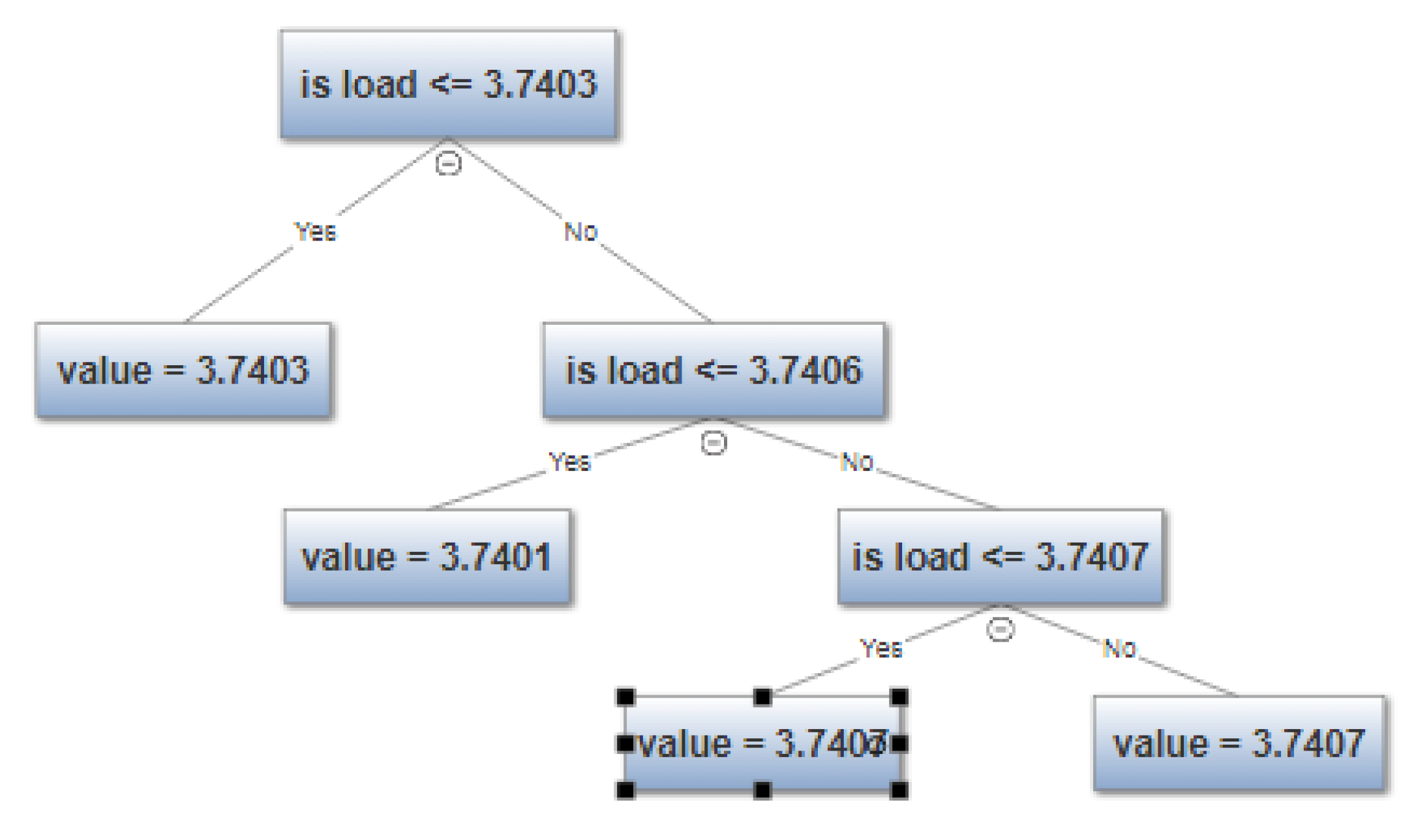
• $D{T}_{trainingSet}$ = {3.7416, 3.7398, 3.7403, 3.7401, 3.7406, 3.7415, 3.7397, 3.7398} and the mean of $D{T}_{trainingSet}$ = 3.7404
• $D{T}_{testSet}$ = {3.7408, 3.74}.

From Equation (6), the SD from the mean for $D{T}_{trainingSet}$ is shown in

Table 2. Standard Deviation for Different Splitting Session of the $D{T}_{trainingSet}$.

$\mathit{D}{\mathit{T}}_{\mathit{t}\mathit{r}\mathit{a}\mathit{i}\mathit{n}\mathit{i}\mathit{n}\mathit{g}\mathit{S}\mathit{e}\mathit{t}}$ at Split 1	SD at Split 1	$\mathit{D}{\mathit{T}}_{\mathit{t}\mathit{r}\mathit{a}\mathit{i}\mathit{n}\mathit{i}\mathit{n}\mathit{g}\mathit{S}\mathit{e}\mathit{t}}$ at Split 2	SD at Split 2	$\mathit{D}{\mathit{T}}_{\mathit{t}\mathit{r}\mathit{a}\mathit{i}\mathit{n}\mathit{i}\mathit{n}\mathit{g}\mathit{S}\mathit{e}\mathit{t}}$ at Split 3	SD at Split 3
3.7416	0.0012	3.7416	0.0012	3.7416	0.00095
3.7398	0.0006	3.7398	0.0006	3.7415	0.00085
3.7403	0.0001	3.7401	0.0003	3.7397	0.00095
3.7401	0.0003	3.7406	0.0002	3.7398	0.00085
3.7406	0.0002	3.7415	0.0011
3.7415	0.0011	3.7397	0.0007
3.7397	0.0007	3.7398	0.0006
3.7398	0.0006

for different split sessions.

• Split 1: The DT was split where the SD is at minimum value, which is at the point where the load value is 3.7403 KW/h. This is S₁ while the remaining members in the $D{T}_{trainingSet}$ will form set S₂ as described in Section 3.3. The S₁ becomes the leaf node while S₂ will go through recursive process of extracting the member set with minimal SE carried out in Split 2 as shown in Table 2.
• Split 2: During this split process, the SD of the remaining dataset in Table 2 will be recalculated to obtain the least SD value. The load value 3.7406 Kw/h with SD 0.0002, being the minimum value among others, is selected as the decision node for further splitting. When the split result is more than one, an average of such result was computed for the leaf node e.g., (3.7398 + 3.7401 + 3.7406)/3 = 3.7401 KW/h.
• Split 3: At this juncture, the corresponding dataset was used to calculate the SD in order to obtain its least SD value. Load values 3.7415 and 3.7398 have the same SD value (0.00085) but the average of the two loads has an approximate value of 3.7407 Kw/h, which will form the decision point to aid the final decision. The final leaf nodes in Figure 11 form the model checked against $D{T}_{testSet}$ for effective testing of the model. $D{T}_{testSet}$ is a new dataset that has never been used during the DT training process and this was used against the training model to obtain a MAE that indicates the predictive performance of the model.

Based on the size of $D{T}_{testSet}$, the same data size was obtained from the DT result in Figure 11 preferably the last unique leaf nodes {3.7407, 3.7401}. Therefore, from Equation (9),

$$\mathrm{MAE}=\frac{\left|3.7407-3.7408\right|+\left|3.7401-3.74\right|}{2}=\frac{0.0001+0.0001}{2}=0.0001$$

In brief, the result of the predictive error (MAE) is a near-zero value for the few datasets considered in this mathematical analysis and compared with the result of the predictive error produced in experiment 2 shown by Figure 15a(ii), we can see that using the cooperative model PSA-DT produces a near-zero predictive error for residential load consumption.

(ii) For Commercial Load Consumption at 99% Confidence level

• $C{L}_{vh}$ = {22.7436, 14.901, 14.9245, 14.9408, 15.1012, 22.9898, 38.9705, 43.2523, 42.1958, 34.702} in Kw/h.
• $\mu =25.6743and\sigma$ = Standard deviation = 1.0486
• $\frac{\sigma }{\sqrt{n}}$ = Standard Error = $\frac{1.0486}{\sqrt{\mathbf{10}}}$ = 0.3316
• $T_{\raisebox{1ex}{$\alpha $}\!\left/ \!\raisebox{-1ex}{$2$}\right.}$ = Confidence Coefficient = $T_{value}$(1-confidence level)/2 = (1 − 0.99)/2 = 0.005 using Equation (2)
• $T_{value}$ (0.005) = 3.250 obtained from T distribution in [35]
• $E_m$ = 3.250 × 0.3316 = 1.0777

Therefore, the confidence interval at 99% confidence degree = 25.6743 ± 1.0777.

• Lower limit with 95% confidence interval = 25.6743 − 1.0777 = 24.5966
• Upper limit with 95% confidence interval = 25.6743 + 1.0777 = 26.752

From the set $C{L}_{vh}$ with a sample load such as 22.7436, 14.901, ..., the load expectation at 95% confidence interval is between 24.5966 Kw/h and 26.752 Kw/h for the class of load users considered. In this situation, using a Monte Carlo experiment, the expected mean generated and this value fall within the computed confidence interval.

The mean loads obtained from the Monte Carlo experiment as $PS{A}_{result}$ = {26.5359, 26.5485, 26.5369, 26.5333, 26.5295, 26.5453, 26.5535, 26.5418, 26.5586, 26.5547} fell within the confidence interval and this result was also split into training and test sets for DT processing using K-fold CV described in Section 3.5.1.

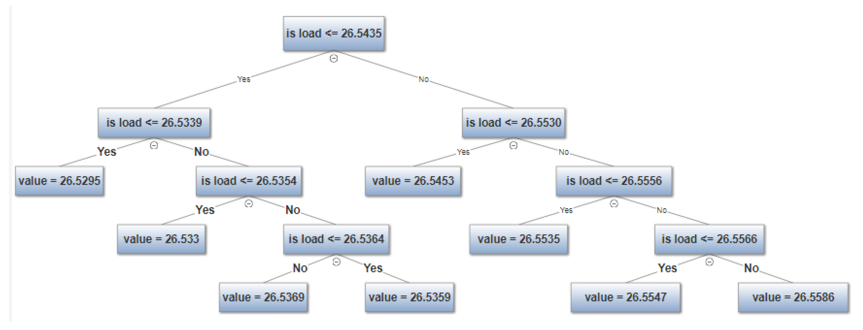
• $D{T}_{trainingSet}$ = {26.5586, 26.5453, 26.5359, 26.5369, 26.5535, 26.5547, 26.5295, 26.5333} and the mean of $D{T}_{trainingSet}$ = 26.5435, which can also be used as the initial root node.
• $D{T}_{testSet}$ = {26.5418, 26.5485}

From Equation (6), SD from the mean for $D{T}_{trainingSet}$ is shown in

Table 3. Standard Deviation for Different Splitting Sessions of the $\mathit{D}{\mathit{T}}_{\mathit{t}\mathit{r}\mathit{a}\mathit{i}\mathit{n}\mathit{i}\mathit{n}\mathit{g}\mathit{S}\mathit{e}\mathit{t}}$.

$\mathit{D}{\mathit{T}}_{\mathit{t}\mathit{r}\mathit{a}\mathit{i}\mathit{n}\mathit{i}\mathit{n}\mathit{g}\mathit{S}\mathit{e}\mathit{t}}$ at Split 1	SD at Split 1	$\mathit{D}{\mathit{T}}_{\mathit{t}\mathit{r}\mathit{a}\mathit{i}\mathit{n}\mathit{i}\mathit{n}\mathit{g}\mathit{S}\mathit{e}\mathit{t}}$ at Split 2	SD at Split 2	$\mathit{D}{\mathit{T}}_{\mathit{t}\mathit{r}\mathit{a}\mathit{i}\mathit{n}\mathit{i}\mathit{n}\mathit{g}\mathit{S}\mathit{e}\mathit{t}}$ at Split 3	SD at Split 3
S1 (initial)
26.5359	0.0020	26.5359	0.0005	26.5359	0.0005
26.5369	0.0030	26.5369	0.0015	26.5369	0.0005
26.5295	0.0044	26.5333	0.0021
26.5333	0.0006
S2 (initial)
26.5586	0.0056	26.5586	0.0030	26.5586	0.0025
26.5453	0.0077	26.5535	0.0021	26.5535	0.0026
26.5535	0.0005	26.5547	0.0009
26.5547	0.0017

for a different split session.

Initially, the average load of 26.5435 Kw/h forms the first root node, as shown in Figure 12. The first decision shows the split result of $D{T}_{trainingSet}$ into S₁ and S₂ based on the validity of the condition that the initial average load is less or greater than the average load of 26.5435.

• S₁ (initial) = {26.5359, 26.5369, 26.5295, 26.5333} was formed when $D{T}_{trainingSet}\le totalmean\left(\mu \right)$.
• S₂ (initial) = {26.5586, 26.5453, 26.5535, 26.5547} was formed when $D{T}_{trainingSet}>totalmean\left(\mu \right).$

• Considering Tree S₁ (initial) with $\mathit{\mu }\left({\mathit{S}}_{\mathbf{1}}\right)=26.5339$:
• Split 1: The split point through S₁ was determined by the least SD with value equal to 0.0006 and the corresponding load value is 26.5333 Kw/h, as shown in Table 3. Therefore, another set of S₁ and S₂ was also formed.
• S₁ = {26.5295} was formed when SD is at its lowest value of 0.0006 and S₁ average ≤ 26.5339 Kw/h.
• S₂ = {26.5359, 26.5369, 26.5333} was formed when SD was at its lowest value of 0.0006 and S₁ average > 26.5339 Kw/h with new S₂ average as 26.5354 Kw/h.
• Split 2: In this section, the split point is at least SD of 0.0005 with a load value of 26.5359 Kw/h and another set of S₁ and S₂ was formed.
• S₁ = {26.533} was formed when SD is at its lowest value of 0.0005.
• S₂ = {26.5359, 26.5369} was formed when SD was at its lowest value of 0.0005 with a new decision node of 26.5364 Kw/h, being an average of S₂.
• Split 3: In this last recursive iteration, the average of S₂ in Split 2 forms the decision node for the final split with an average of the remaining member set because they both have the same SD value of 0.0005.

• Considering Tree S₂ (initial) with $\mathit{\mu }\left({\mathit{S}}_{\mathbf{2}}\right)=26.5530$:
• Split 1: The split point through S₁ was determined by the least SD with value equal to 0.0005 and the corresponding load value is 26.5535, as shown in Table 3. Therefore, another set of S₁ and S₂ was formed.
• S₁ = {26.5453} was formed and S₂ = {26.5586, 26.5535, 26.5547} was also formed with new S₂ average as 26.5556 Kw/h forming the next decision node, as shown in Figure 12.
• Split 2: In this section, the split point is at least SD of 0.0009 with a load value of 26.5547 Kw/h and another set of S₁ and S₂ was formed.
• S₁ = {26.5535} was formed, and S₂ = {26.5586, 26.5547} was also formed with a new decision node of 26.5566 Kw/h, being an average of S₂.
• Split 3: In this last recursive iteration, the previous set S₂ forms the leaf node, as shown in Figure 12.

Based on the size of $D{T}_{testSet}$, same data size was obtained from the DT result in Figure 12 preferably the last unique leaf nodes {26.5586, 26.5547}. Therefore, from Equation (9),

$$\mathrm{MAE}=\frac{\left|26.5418-26.5586\right|+\left|26.5485-26.5547\right|}{2}=\frac{0.0168+0.0062}{2}=0.0115$$

From the MAE result obtained from the mathematical analysis of a commercial load using cooperative PSA-DT, we can also see the near-zero predictive result. This result also falls within the predictive error shown in Figure 15b(ii).

4. Evaluation of PSA-DT for Short-Term Load Forecasting towards Economic Sustainability

4.1. Experimental Setup for Smart Grids

As described earlier, short-term load forecasting corresponds to predictions ranging from one minute to one week ahead. In this research, data collected include residential, commercial and industrial loads. The residential and commercial loads were from a location in Texas, USA, obtained as secondary data from open energy information [8], and industrial data were collected from Terni Energy in Germany [11]. A brief overview of the data layout, shown in Figure 13, is the snapshot of the various data meant for different classes of electricity consumers. Each electricity consumer serves as an entry point to the PSA-DT model, as shown in Figure 7. These time-series loads were then stored in the data repository after being processed via the knowledge-based system. During electricity forecast planning by the grid owners, historical records stored in this repository were fetched by the model to make its prediction.

The major raw input data fed into the designed model were the time series load data for different categories of data collected. The predictive problem was approached by systematically following the PSA-DT pseudo-code in Figure 10. During the implementation, several libraries and software in addition to PANDAS for data analysis were used. These are matplotlib for data visualization, sklearn package, a repository of diverse machine learning algorithms where the DT model and other algorithms were obtained for the experiments. In addition, scipy is used for both descriptive and inferential statistics such as mean, variance and standard deviation. Using the random sample experiment, a high confident level estimated mean was generated prior to final decision-making via the use of a DT model. This forms the basis of the model explanation in this article.

In summary, Feinberg and Genethliou [21] advised researchers to investigate several applications of the developed model and also argued that there is no single model or algorithm that is superior for all utility firms. This is due to variation in the consumption pattern of different categories of consumers at different locations. In addition, variation includes the geographical, climatic, economic and social attributes. In selecting the most appropriate algorithm, the utility will require to test it on real data. According to Feinberg [21], there is no system that could predetermine which forecasting technique is most accurate for given load data. Nevertheless, every model needs to be well-trained and tested over the load data.

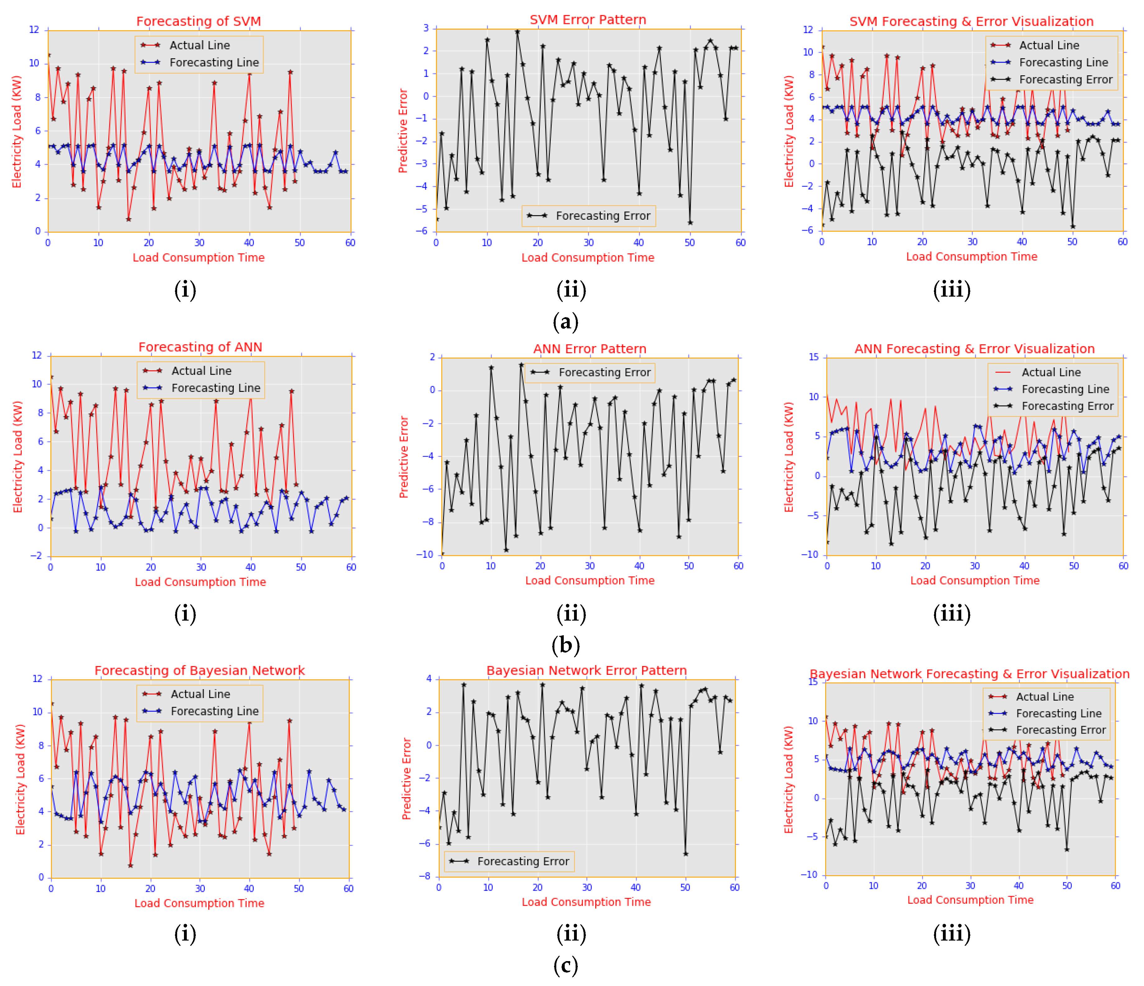
4.2. Experiment 1: Electric Load Forecasting with Classical Models on Residential Load Consumption

In Figure 14a–c, the residential load consumption in Kw/h shown on the y-axis and the hourly consumption time on the x-axis were used during the various experimental setups. The load was predicted in parallel with the actual load using the forecasting line till the 50th hour, as shown in these sections’ figures. The 51st and 60th hour being the ten step forecasting horizon that depicts the future predictions for each of the classical models based on the residential data in Figure 13a. The aim is to verify the predictive performance in terms of reduced MAE in each model considered. The models exhibited differences in their predictive error, as shown in Figure 14a(ii), Figure 14b(ii), and Figure 14c(ii) for SVM, ANN and Bayesian networks (BN), respectively. Based on the behaviour of the three models, the following reasoning analysis guides the actions of future electricity consumption planners in their decision processes.

• Decision-making: The sampled qualitative analysis between the 51st and 60th hour for this experiment gave a corresponding answer to some of the questions asked.

• (Question) Q1: What is happening to the predictive behaviour?
• (Answer) A1: The predictive error in SVM is reduced with peak values ranging between −5.8 kw/h and 3.0 kw/h; BN predictive error is slightly higher than SVM error with a value between −6.8 kw/h and 3.8 kw/h; and predictive error from ANN is relatively higher than the results of the other classical models and ranges from −9 kw/h to 1.8 kw/h.
• Although the SVM could predict slightly better compared with the other classical models considered in terms of low predictive errors, its predictive performance can still be improved with the PSA-DT model. Although BN could predict up to 6 kw/h for an actual load of 10 kw/h, as shown in Figure 14c(i), the predictive error was still higher than the SVM predictive error. In addition, the ANN forecasting result in Figure 14b(i) could not fit the actual load for different load consumption periods. This irregularity was because large amounts of data were needed to train the ANN model for effective predictions. Therefore, these shortfalls contributed to the high predictive error generated by the ANN model in Figure 14b(ii).

• Q2: Why is it happening?
• A2: Inability of the forecasting models to predict the actual electricity load consumption accurately; this proposition can be seen clearly in Figure 14a(i), Figure 14b(i), and Figure 14c(i), meant for SVM, ANN and BN, respectively, where their forecasting lines in blue did not “fit” their corresponding actual load lines in red. Overall, there was an under-estimation.

• Q3: What can be done about it?
• A3: The forecasting error can be improved by deploying an effective cooperative model for the predictive analysis.

• Q4: What will happen next?
• A4: The SVM model tends to predict well in terms of low predictive error depicted by Figure 14a(ii), with a predictive error value of −5.8 kw/h to 3.0 kw/h when compared with the predictive error result of BN and ANN.

In Figure 14a(i), SVM predicts the future load consumption as between 4 Kw/h and 5 Kw/h even when the actual load at some approximate time such as 12 h, 22 h and 32 rises to 10 Kw/h and sometimes reduces to as low as 1 kw/h. In brief, we can also deduce that the predictive result rises and drops with respect to increases and decreases in actual load consumption, respectively. To address the results of high predictive errors produced by the classical models, the use of an uncertainty model could be of a great assistance for more reliable electricity load predictions and near-zero predictive errors.

However, one might have noticed the fluctuating nature of the predictive error over time; this is due to the unpredictable nature of the load consumption feature, implying that there will be a great need for a probabilistic model such as PSA-DT that can handle the uncertain conditions better.

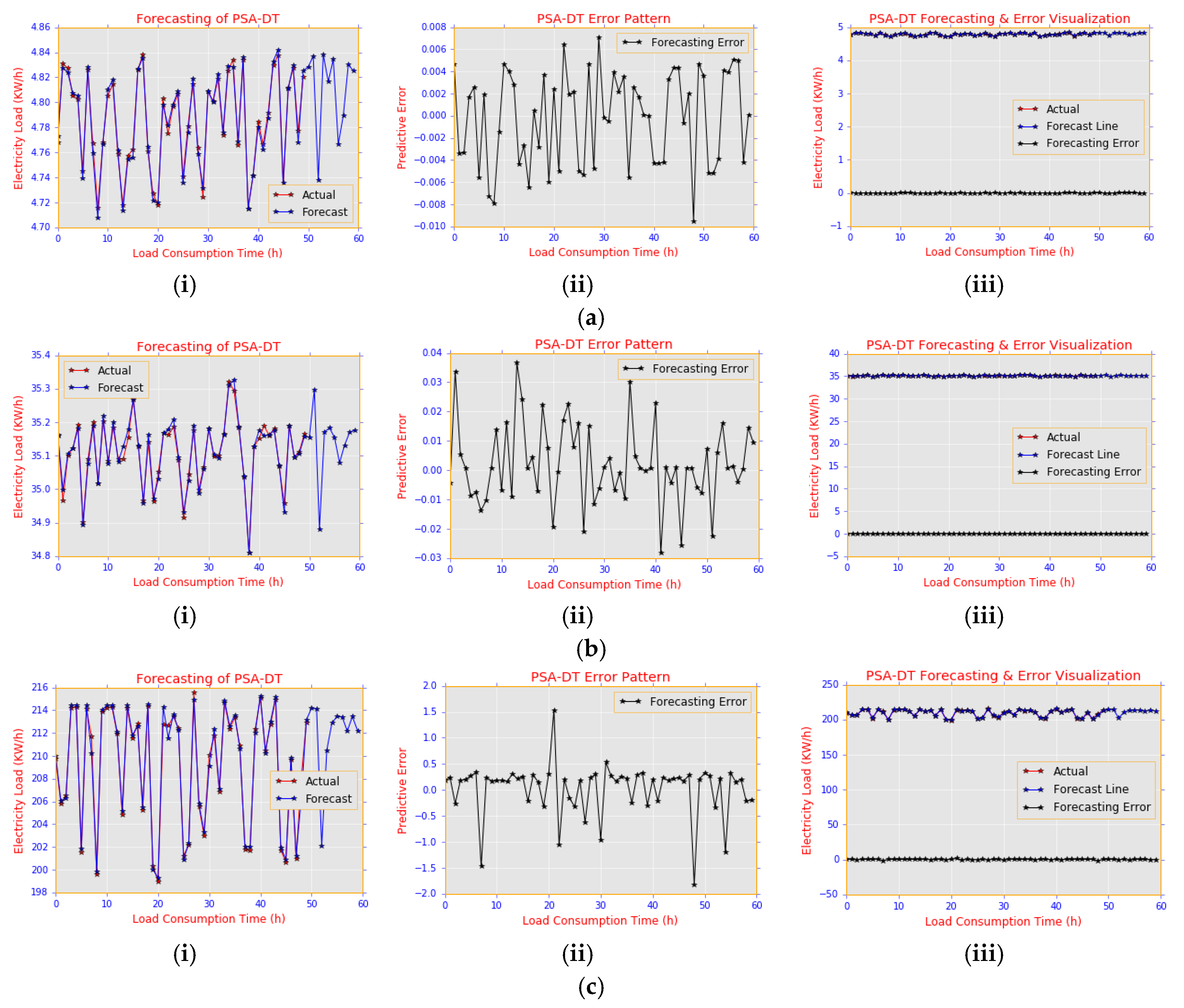
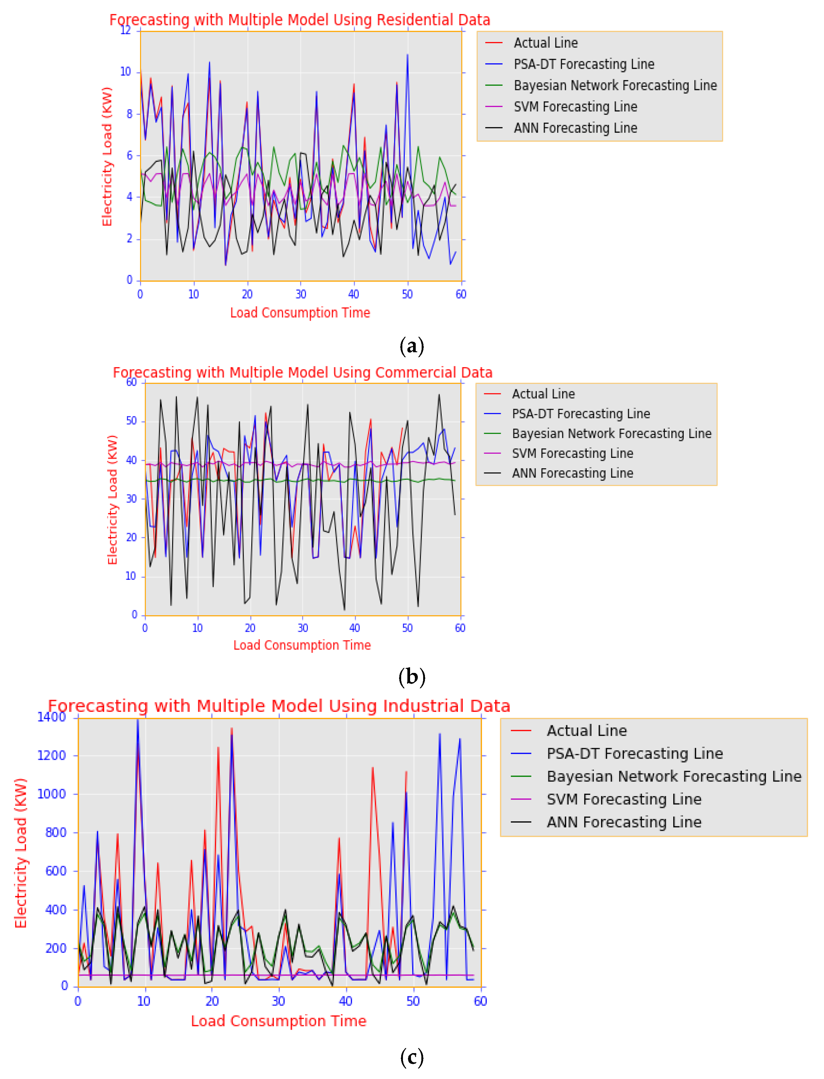
4.3. Experiment 2: Electric Load Forecasting with PSA-DT on Three Classes of Consumers in Smart Homes

The objective of this test and the results obtained, as shown in Figure 15a–c, is to affirm effectiveness in the predictive ability of PSA-DT in terms of the low predictive error computed using Equation (9) and comparing the PSA-DT predictive error and the classical model error.

• Decision-making: Sampled qualitative analysis between load consumption Hour 0 to Hour 50 and beyond.

• Q1: What is happening to the predictive behaviour?
• A1: The predictive error for the PSA-DT model was reduced to a range of −0.01 to 0.01 for residential load consumption, as shown in Figure 15a(ii); error values ranged from −0.04 to 0.04 for a commercial load user category in Figure 15b(ii) and −1.5 to 0.5 for an industrial load user. The negative predictive error value occurred because under-prediction and over-prediction produce a positive predictive error value. Since this error is extremely small compared to the value generated by the classical model shown in experiment Figure 14a–c(ii), the forecasting result generated by PSA-DT model tends towards higher accuracy than the result obtained from the classical model for all classes of users being considered.

• Q2: Why is it happening?
• A2: This predictive error reduction occurred because of the cooperative nature of the PSA-DT model formed by combining the merits of both PSA and the DT model described in Section 3. Because of the uncertain nature of electricity load consumption, we obtained the expected mean load with high confidence value via the Monte Carlo experiment before passing the result into a DT for effective learning and predictions.

• Q3: What can be done about it?
• A3: To maintain the efficiency of the cooperative model, data used for such predictions can be obtained with a low time interval, less than an hourly data interval. In addition, the classical models such as ANN and SVM can be improved by acquiring more data for effective learning of the model and for better representation of the future data point in the training data.

• Q4: What will happen next?
  A4: Deploying this predictive model during future load planning within an SG has huge potential to yield an effective forecasting result with high confidence of low predictive error.

This experiment shows the different forecasting abilities and the forecasting error of the cooperative PSA-DT model when used for different classes of user load consumption, such as residential, commercial and industrial.

In this section, the result of Figure 15a(i) depicts how well the forecast load fitted the actual residential load with near-zero error, as shown in Figure 15a(ii). With the near-zero error of value ranging from −0.01 to 0.007, a periodic peak error value was obtained at 10 h, 22 h and 29 h. According to Figure 15a(ii), the predictive error is still lower than the error results of the classical model used for residential load consumption. Moreover, these possibilities occurred as a result of effective PSA-DT model usage with low standard deviation from the mean load in residential electricity load consumption.

This research deduced from Figure 15b(ii) that the result of the cooperative predictive model produces a predictive error close to zero with value ranges from −0.03 to 0.04 and the peak error found at 2 h, 12 h, 20 h, 23 h and 40 h, to mention a few. This reduction aids the model predictive abilities for economic sustainability. Though the standard deviation from the mean load is slightly higher than the corresponding residential load consumption, the predictive error remained within the range value, which is lower than the predictive error of the classical model when used by the same load user category as show in

Table 4. (a) Predictive Errors from SG Categories of Users using PSA-DT and SVM; (b) predictive Errors from SG Categories of Users using PSA-DT and BN; and (c) predictive Error Comparison from SG Categories of Users using PSA-DT and ANN.

(a)
Predictive Model	Smart-Grid Data (User Category)	Hourly Load Data Size	Training Size (%)	Test Size (%)	Predictive Error (MAE) for PSA-DT	Predictive Error (MAE) for SVM
PSA-DT and SVM	Residential	100	60	40	0.0018	0.0105
			80	20	0.002	0.0100
		200	60	40	0.0028	0.007
			80	20	0.002	0.02
		500	60	40	0.0032	0.0463
			80	20	0.0038	0.0336
	Commercial	100	60	40	0.0093	0.05
			80	20	0.0095	0.078
		200	60	40	0.0093	0.0544
			80	20	0.0093	0.0715
		500	60	40	0.0150	0.1059
			80	20	0.0129	0.08
	Industrial	100	60	40	0.2375	1.2713
			80	20	0.2345	1.9485
		200	60	40	0.20438	1.3151
			80	20	0.2185	1.6672
		500	60	40	0.4369	1.8399
			80	20	0.4252	4.062
(b)
Predictive Model	Smart-Grid Data (User Category)	Hourly Load Data Size	Training Size (%)	Test Size (%)	Predictive Error (MAE) for PSA-DT	Predictive Error (MAE) for BN
PSA-DT and BN	Residential	100	60	40	0.0018	0.0028
			80	20	0.002	0.0045
		200	60	40	0.0028	0.0075
			80	20	0.002	0.00475
		500	60	40	0.0032	0.0053
			80	20	0.0038	0.0109
	Commercial	100	60	40	0.00925	0.011
			80	20	0.0095	0.0145
		200	60	40	0.0093	0.0178
			80	20	0.0093	0.0193
		500	60	40	0.0150	0.0315
			80	20	0.0129	0.0323
	Industrial	100	60	40	0.2375	1.3978
			80	20	0.2345	1.996
		200	60	40	0.204375	0.653875
			80	20	0.2185	0.7785
		500	60	40	0.4369	1.1663
			80	20	0.4252	1.7514
(c)
Predictive Model	Smart-Grid Data (User Category)	Hourly Load Data Size	Training Size (%)	Test Size (%)	Predictive Error (MAE) for PSA-DT	Predictive Error (MAE) for ANN
PSA-DT and ANN	Residential	100	60	40	0.0018	0.0118
			80	20	0.002	0.013
		200	60	40	0.0028	0.0124
			80	20	0.002	0.0235
		500	60	40	0.0032	0.0569
			80	20	0.0038	0.0466
	Commercial	100	60	40	0.00925	0.0643
			80	20	0.0095	0.086
		200	60	40	0.0093	0.0575
			80	20	0.0093	0.078
		500	60	40	0.0150	0.1283
			80	20	0.0129	0.0904
	Industrial	100	60	40	0.2375	2.3153
			80	20	0.2345	2.0225
		200	60	40	0.204375	1.558
			80	20	0.2185	1.6768
		500	60	40	0.4369	2.2818
			80	20	0.4252	4.0605

.

In Figure 15c, the predictive error was a little higher between −1.9 and 1.6. This peak value was achieved occasionally in Figure 15c(ii) at 8 h, 21 h, 22 h and 49 h, but it is better than the predictive result produced by other classical models when used for industrial load prediction with the detailed experiment shown in Table 4. However, this was a result of high standard deviation in the historical load for industrial electricity load consumption.

Generally, the predictive result of the experiment (Figure 15a–c) was extrapolated after the 50th load data in order to predict the next few hours between the hours of 51 and 60 for each of the experiments. The corresponding reduced near-zero predictive error in Figure 15a–c(ii) shows how well the cooperative PSA-DT model can predict using interpolated results ranging from 0 to 50th load data value and after the 50th load data value.

From the visualization result, the blue line depicts the forecast load, which almost “maps” the red line that shows the actual load with a near-zero forecasting error in Figure 15a–c(ii). In addition, ranging from the residential load to the industrial load, the analytical plots in experiments 1 and 2 denote that different users’ categories have different load consumption patterns and the cooperative PSA-DT can predict the consumption to a high degree of predictive accuracy with reduced forecasting error, but it is notable that the level of errors also varies among load categories considered owing to variations in their load standard deviation from the mean load.

4.4. Performance Evaluation of Electric Load Forecasting with PSA-DT and Classical Models

Another fascinating observation was the cooperative model fitting the actual load consumption compared to other models at load times up to the 50th hour and till the 60th hour for future prediction, as shown in Figure 16a–c. In the residential load category, one could see in residential load consumption the “overlap” of the red and blue lines depicting the actual and PSA-DT forecasting line in Figure 16a, but, in Figure 16c, the PSA-DT could not fit very well from the hour 20 to hour 22 and hour 44 to hour 46. This was a result of wide deviation of the load from the mean load in industrial load with a value of 395.4969 compared to the residential load consumption having a mean deviation of 2.9295.

This research made differential analyses in terms of forecasting error levels between PSA-DT and the classical models. The experimental result in Table 4a–c shows the various predictive error results of PSA-DT compared with each of the classical models for different hourly load data, training and test sizes. In each table and for each of the SG user categories, the corresponding experiment produced different predictive errors for PSA-DT and each of the classical models. In a more elaborate form, Table 4a–c shows the predictive error comparison between PSA-DT and SVM, PSA-DT and BN and finally, PSA-DT and ANN for different categories of load users with different hourly load data sizes of 100, 200 and 500 in each category. We also considered different percentages of training and test sizes of 60% and 40%, 80% and 20%, as detailed in the tables. Going through each of these variations and performing the corresponding experiment, different predictive error values were obtained, as highlighted in the tables.

Table 4a shows the comparison between PSA-DT and SVM in terms of their predictive errors. The tabular result aids a quick comparison using different variations of datasets with diverse training and test sets for all the classes of electricity user consumption. In each of the experiments and having obtained the MAE, using Equation (9), for both PSA-DT and SVM with different variations in training and test set sizes, the MAE of the PSA-DT is lower than the SVM results in all the experiments shown in Table 4a. These differences explain how PSA-DT outperforms SVM in predicting the future electricity load consumption in smart homes. We can deduce that, for each of the experiments in Table 4a, the predictive error value in PSA-DT is lower than the corresponding result from SVM. In the residential user category, using 100 data size in conjunction with 60% training and 40% test data size, the corresponding predictive error of PSA-DT is 0.0018, while the result of the SVM model is 0.0105. In the commercial load user category, the predictive error value of PSA-DT is 0.0093, SVM is 0.05 and also in the industrial user group, the predictive error of PSA-DT is 0.2375 and that of SVM is 1.2713.

Experimental results in Table 4b show the different variations of the training and test set for various hourly load sizes of 100, 200 and 500 used by each user category. In the tabular analysis, there is still a high level of significant differences between PSA-DT and BN predictive errors. Considering the data size of 200 in the commercial user category with training and test sizes of 80% and 20% respectively, the PSA-DT predictive error was 0.0093, while that of BN was 0.0178. In addition, in the residential category of the same data size, the PSA-DT predictive error was 0.002 while that of BN was 0.00475. This gave the PSA-DT improved performance over BN by generalising the predictive results of PSA-DT performance over BN in each of the experiments.

In Table 4c, PSA-DT predictive abilities were also benchmarked against ANN, as shown by the various experiments. In addition to the numerical justification from Table 4a,b, we can also see clearly the differences in PSA-DT and ANN predictive error values. The predictive error in an industrial hourly load data size of 500 with training and test size of 60% and 40% resulted in 0.4369 and 2.2818 for PSA-DT and ANN respectively. In this regard, the table presented a clear difference in their performance for various observations among different classes of electricity consumers.

It is worth noting that the huge predictive errors in the industrial user category compared to the residential and commercial categories were due to a large statistical variance in the industrial dataset, as shown by sample data in Figure 13c. However, increasing the size of the dataset can result to further decrease in the predictive error.

Therefore, it was observed that the cooperative probabilistic scenario analysis with DT in forecasting future electricity load consumption for smart homes is more accurate, as it produces a near-zero predictive error for all the categories of users considered in this research, as shown in Table 4. The experimental results show that various classes of load, such as residential, commercial and industrial, of diverse data size, behave differently revealing sustainable economic consumption patterns.

Hence, the PSA-DT model could predict the future load more accurately for smart-homes with a low predictive error in relation to the analysed data set and the particular structure of the classical models adopted in BN, SVM and Multilayer Perceptron (MLP), which is a class of feedforward Artificial Neural Network, considered in this research.

5. Concluding Remarks

This research was built on Monte Carlo PSA complemented with a DT model depicted by the model framework in Figure 7. The critical analysis was conducted as shown in experiments 1 and 2 and the tabular results in Table 4 on the cooperative PSA-DT model performance with emphasis on reducing the predictive error that can result in high accuracy for electricity load forecasting in an SG. This will aid effective planning for sustainable economic development, especially when used by SG owners. Such accurate forecasting will minimise wastage by assisting utility managers to know the possible total amount of electricity that will be supplied to various smart homes for future electricity consumption.

The cooperative model for sustainable demand planning in an SG was developed using a probabilistic simulation of the load to obtain a list of cumulative loads via successive random generation. Such loads generate a high level of confidence interval for their expected mean acceptability. Following the model flow in Figure 8, the accepted list was fed into the DT model, trained and fitted; it finally predicted the future load consumption.

Overall, PSA-DT proved more efficient than the state-of-the-art model by producing a near-zero predictive error for the different categories of users considered, as shown in the various experiments in Section 4. This implies that such a probabilistic model will enhance accurate decision-making when planning for future electricity load consumption in an SG.

However, future prediction of short-term loads is affected by various factors. Therefore, consideration should be given to some of the factors, such as weather parameters, number of customers in different categories, the appliances being used in those areas and electric load (in turn reflecting consumers’ personal characteristics, e.g., age, economic and demographic data, as well as appliances sales data and other related factors). Other factors such as days of the week and time of the year should also be considered.

In summary, future research activities might focus on the effect of weather parameters such as temperature, pressure, relative humidity and wind speed, which are critical factors in the load consumption in an SG using the collaborative model. It will be valuable to analyse the effect of each of the weather parameters on the consumer electricity load consumption, and to determine how PSA-DT can be used in the prediction of load consumption for improved decision-making by SG electricity planners for smart homes.

References

- Xiao, L.; Wang, J.; Hou, R.; Wu, J. A combined model based on data pre-analysis and weight coefficients optimization for electrical load forecasting. Energy 2015, 82, 524–549. [Google Scholar] [CrossRef]
- Li, H.; Guo, S.; Li, C.; Sun, J. A hybrid annual power load forecasting model based on generalized regression neural network with fruit fly optimization algorithm. Knowl.-Based Syst. 2012, 37, 378–387. [Google Scholar] [CrossRef]
- Islam, B.; Baharudin, Z.; Raza, Q.; Nallagownden, P. A hybrid neural network and genetic algorithm based model for short term load forecast. Res. J. Appl. Sci. Eng. Technol. 2014, 7, 2667–2673. [Google Scholar] [CrossRef]
- Yang, Y.; Wu, J.; Chen, Y.; Li, C. A New Strategy for Short-Term Load Forecasting; Hindawi Publishing Corporation: Cairo, Egypt, 2013. [Google Scholar]
- Ko, C.-N.; Lee, C.-M. Short-term load forecasting using SVR (support vector regression)-based radial basis function neural network with dual extended Kalman filter. Energy 2013, 49, 413–422. [Google Scholar] [CrossRef]
- Almeshaiei, E.; Soltan, H. A methodology for electric power load forecasting. Alex. Eng. J. 2011, 50, 137–144. [Google Scholar] [CrossRef]
- Australian Energy Market Operator. Forecast Accuracy Report 2016; For The National Electricity Forecasting Report; Australian Energy Market Operator: Melbourne, Australia, 2016. [Google Scholar]
- US Electricity Operating Data. U.S. ELECTRIC SYSTEM OPERATING DATA. Available online: https://www.eia.gov/beta/realtime_grid/#/data/graphs?end=20170402T00&start=20170326T00 (accessed on 24 February 2017).
- Day, P.; Fabian, M.; Noble, D.; Ruwisch, G.; Spencer, R.; Stevenson, J.; Thoppay, R. Residential power load forecasting. Procedia Comput. Sci. 2014, 28, 457–464. [Google Scholar] [CrossRef]
- Fan, C.; Xiao, F.; Wang, S. Development of prediction models for next-day building energy consumption and peak power demand using data mining techniques. Appl. Energy 2014, 127, 1–10. [Google Scholar] [CrossRef]
- OpenEI. Commercial and Residential Hourly Profiles for all TMY3 Locations in the United State. Available online: http://en.openei.org/datasets/dataset/commercial-and-residential-hourly-load-profiles-for-all-tmy3-locations-in-the-united-states (accessed on 25 December 2016).
- Kassakian, J.G.; Schmalensee, R.; Desgroseilliers, G.; Heidel, T.D.; Afridi, K.; Farid, A.M.; Grochow, J.M.; Hogan, W.W.; Jacoby, H.D.; Kirtley, J.L.; et al. The Future of the Electric Grid: An Interdisciplinary MIT Study; Massachusetts Institute of Technology: Cambridge, MA, USA, 2011. [Google Scholar]
- OpenEI. Smart Energy Data: Terni Energy Consumption Profiles. Available online: https://data.lab.fiware.org//dataset/b6ac9ad2-7b9e-4247-a785-81a88021995c/resource/3994b4ba-788a-4def-852f-043c71a20084/download/ternienergyconsumptionprofilecustomerindustrial1.csv (accessed on 24 November 2016).
- Soliman, S.A.; Persaud, S.; El-Nagar, K.; El-Hawary, M.E. Application of least absolute value parameter estimation based on linear programming to short-term load forecasting. Int. J. Electr. Power Energy Syst. 1997, 19, 209–216. [Google Scholar] [CrossRef]
- Badar, E.; Islam, U. Comparison of conventional and modern load forecasting techniques based on artificial intelligence and expert systems. Int. J. Comput. Sci. Issues 2011, 8, 504–513. [Google Scholar]
- Soliman, S.A.; Al-Kandari, A.M. Electrical Load Forecasting; Elsevier: Amsterdam, The Netherlands, 2010. [Google Scholar]
- Ismail, M.M.; Hassan, M.M. Artificial neural network based approach compared with stochastic modelling for electrical load forecasting. In Proceedings of the 2013 5th International Conference on Modelling, Identification and Control (ICMIC), Cairo, Egypt, 31 August–2 September 2013; pp. 112–118. [Google Scholar]
- Hahn, H.; Meyer-Nieberg, S.; Pickl, S. Electric load forecasting methods: Tools for decision making. Eur. J. Oper. Res. 2009, 199, 902–907. [Google Scholar] [CrossRef]
- Chen, B.-J.; Chang, M.-W.; Lin, C.-J. Load forecasting using support vector Machines: A study on EUNITE competition 2001. IEEE Trans. Power Syst. 2004, 19, 1821–1830. [Google Scholar] [CrossRef]
- Tepedino, C.; Guarnaccia, C.; Iliev, S.; Popova, S.; Quartieri, J. A forecasting model based on time series analysis applied to electrical energy consumption. Int. J. Math. Model. Methods Appl. Sci. 2015, 9, 432–445. [Google Scholar]
- Feinberg, E.A.; Genethliou, D. Load forecasting. In Applied Mathematics for Restructured Electric Power Systems; Springer: Berlin, Germany, 2006; pp. 269–285. [Google Scholar]
- Koo, B.G.; Lee, S.W.; Kim, W.; Park, J.H. Comparative study of short-term electric load forecasting. In Proceedings of the 2014 5th International Conference on Intelligent Systems, Modelling and Simulation, Langkawi, Malaysia, 27–29 January 2014; pp. 463–467. [Google Scholar]
- Cheepati, K.R.; Prasad, T.N. Performance comparison of short term load forecasting techniques. Int. J. Grid Distrib. Comput. 2016, 9, 287–302. [Google Scholar] [CrossRef]
- Atmaca, H. The comparison of fuzzy inference systems and neural network approaches with ANFIS method for fuel consumption data. In Proceedings of the Second International Conference on Electrical and Electronics Engineering Papers ELECO, Bursa, Turkey, 7–11 November 2001; Volume 6, pp. 1–4. [Google Scholar]
- Ismail, Z.; Mansor, R. Fuzzy logic approach for forecasting half-hourly Malaysia electricity. In Proceedings of the 31st International Symposium On Forecasting, Prague, Czech Republic, 26–29 June 2011. [Google Scholar]
- Wu, L.; Shahidehpour, M. A hybrid model for integrated day-ahead electricity price and load forecasting in smart grid. IET Gener. Transm. Distrib. 2014, 8, 1937–1950. [Google Scholar] [CrossRef]
- Yoe, C. Probabilistic scenario analysis. Princ. Risk Anal. 2011, 399–420. [Google Scholar]
- Bessa, R.J.; Trindade, A.; Silva, C.S.; Miranda, V. Probabilistic solar power forecasting in smart grids using distributed information. Int. J. Electr. Power Energy Syst. 2015, 72, 16–23. [Google Scholar] [CrossRef]
- Bood, R.P.; Postma, T.J.B.M. Scenario Analysis as a Strategic Management Tool; University of Groningen: Groningen, The Netherlands, 1998; pp. 1–38. [Google Scholar]
- Alemohammad, S.H.; Ardakanian, R.; Karimi, A. A framework for modelling probabilistic uncertainty in rainfall scenario analysis. arXiv preprint 1995, arXiv:1304.4302, 1–8. [Google Scholar]
- Analysis, S. Chapter 6 Probabilistic Approaches: Scenario Analysis, Financial Times. 1–61.
- Ben-Naim, A. Entropy, Shannon’s measure of information and Boltzmann’s H-theorem. Entropy 2017, 19, 48. [Google Scholar] [CrossRef]
- Sreerama, K.M. Automatic construction of decision trees from data: A multi-disciplinary survey. Data Min. Knowl. Discov. 1998, 2, 345–389. [Google Scholar]
- We, X. Methods for Statistical Data Analysis with Decision Trees; Sobolev Institute of Mathematics: Novosibirsk, Russia, 2003. [Google Scholar]
- UF Department of Statistics. Statistical Tables; UF Department of Statistics: Gainesville, FL, USA, 2002; Volume II, pp. 1–26. [Google Scholar]