Analysis of Energy Efficiency Measures and Retrofitting Solutions for Social Housing Buildings in Spain as a Way to Mitigate Energy Poverty

Abstract

Energy poverty is a common issue in social housing all over Europe, with a harder impact in Southern European countries. Social housing buildings play an important role in energy poverty. They are usually owned and managed by public institutions and usually share common characteristics and issues. Behavioural changes and energy retrofitting are interesting paths forward but some solutions do not fit well in this type of housing due to socioeconomic reasons. This paper makes a thorough analysis of possible energy efficiency measures in social housing buildings, characterizing them by energy and economic savings and investment and proposing different methods of prioritization. A rational approach of behavioural and retrofitting solutions that best fit into this particular housing type is delivered, with the aim to increase the thermal comfort of the residents and mitigate the energy poverty issue. Results show that there is a wide range of domestic efficiency measures to be applied in this type of dwellings at none or low costs, bringing annual savings per average dwelling of about 510 €/year (55% of initial energy costs) including measures both at domestic level, and at building level with a final aggregated payback of the investments to be about 1.5 years.

1. Introduction

Energy vulnerability is a common risk in social housing due to the low income level of the families that fall back on this type of social service [1]. Bergasse et al. [2] define energy poverty as the level of a household income below the minimum energy costs that are necessary to achieve a satisfactory living condition within a dwelling. Hence, energy poverty is a global issue [3] that can be considered a particular case of poverty, and it is basically determined by several factors, such as a low ratio of income and annual energy expenditure, the building energy efficiency and other behavioural and occupant attitudes to achieve a given level of comfort [4].

There are two ways of addressing the issue of energy poverty. One way is by reporting energy poverty cases to assess their eligibility for public aids meant to help families to temporarily cover their energy costs, mainly in winter. Social workers play an important role in identifying and certifying energy poverty issues as stated by Scarpellini et al. [5] and Llera et al. [6]. This is a short-term temporary solution, but the issue remains unsolved and will likely turn up again next winter season.

The second way is by finding corrective solutions to their unaffordable energy consumptions, by reducing their energy expenditure while keeping, or even increasing, their thermal comfort level. This approach provides a solution to the energy vulnerability issue and reduce social and health inequalities [7] joining the benefits of sustainable energy policy with low-income housing policy [8]. This is a long-term definitive solution, which implies acting in the elements, systems and activities that consume energy in a dwelling. The cost of this second way has to be put against the cost of maintaining continuous palliative aids to vulnerable households and the inherent economic charges to the National Public Health System due to tenants’ health problems, air pollution and other environmental burdens [9].

A natural source of improvement is the compulsory adaptation to more environmentally stringent policies as Directive 2010/31/EU [10] is being transposed and applied to existing buildings that are subject to major renovation. This level of changes is definitely too slow, especially when social welfare and health are concerned. Social housing renewal would also take too long and, thus, retrofitting current buildings seems to be the best path forward [11].

The main energy consumptions in a residential dwelling are thermal energy for heating and domestic hot water (DHW), and electricity for lighting and home appliances. Among them, the largest is usually the energy consumption for heating. This is particularly an issue in Southern Europe, despite more favourable climatic conditions due to the poorer insulation of the buildings [12], the inefficiency of the heating equipment in use and the lack of knowledge about efficient energy use at home [13]. This issue has been particularly acknowledged in the “Winter Package” by the European Commission [14], and by authors including Tirado-Herrero and Bouzarovsky [15]. Energy-vulnerable households face not only a problem of comfort but a problem of health [16].

Spain’s social housing system relies mainly on freehold tenure [17], with a short amount of publicly owned buildings [18]. A freehold tenure means a permanent and absolute tenure of the property with freedom to dispose of it at will, as opposed to a leasehold in which the property reverts back to the owner after the lease period has expired. This paper focuses on the second type, which plays a crucial role in offering low-cost, affordable access to a house for vulnerable families [19]. This type of social housing in Spain is a particular kind of housing that share common characteristics that make it homogeneous to some extent, and, for the purpose of this study: they are usually urban blocks of individual apartments owned by a Municipality, and being managed by the owning Public Body or by a subcontracted public or private company [20]. Apartments are allocated to families at an advantageous rent according to a number of requirements, among which are low level of incomes and risk of social vulnerability [21]. Buildings are usually well maintained but often they are old and built with poor construction materials and standards [22].

The case of public social housing represents a special situation because residents have neither the awareness nor the economic capacity to undertake any serious investment on building retrofit and efficient equipment replacement [23]. In addition, often, they are not the owners of the dwellings and are not entitled to make any major modification on the facilities, hindering any investment attempt [23]. In this case, a combined effort of social building users and property is needed to carry out holistic energy saving actions.

This paper quantifies and analyses a high number of energy efficiency measures in buildings, and recommendations about the best way to filter out, order and prioritize energy saving actions in a representative sample of social housing dwellings in Spain, using energy simulation tools and economic criteria, unlike other tested systems like Mikucioniené et al. [24]. The methodology proposed can be applied in similar cases of the same type of buildings and users. In the same way, limitations of these tools to evaluate the implementation of the recommended set of measures are described and results are reviewed and corrected accordingly.

2. Methodology

Computer-aided energy simulation is an interesting tool to assess the effect on energy performance of different possible efficiency measures due to the low cost, high accuracy and great versatility of this method, as illustrated by Altan et al. [25]. The methodology proposed is based on the characterization of a number of possible energy efficiency measures by means of energy simulation tools, and the right selection and priority setting based on economic terms for this type of buildings in a real representative case study, similar to the procedure followed by Sadineni et al. [26] and Ascione et al. [27]. The methodology presented is an alternative to the one presented by Tan et al. [28], but focusing in immediate effects at the possible lowest cost, to address the urgent issue of families undergoing energy poverty issues. It prioritizes economic factors on top of purely environmental (similar to Pombo et al. [29]) since the perceived economic benefits are key drivers of action by most decision makers, and energy poverty is mainly an economic problem [30]. A single dwelling has been taken as the analysis unit since this is the unit of most energy poverty studies, in line with Walker et al. [31].

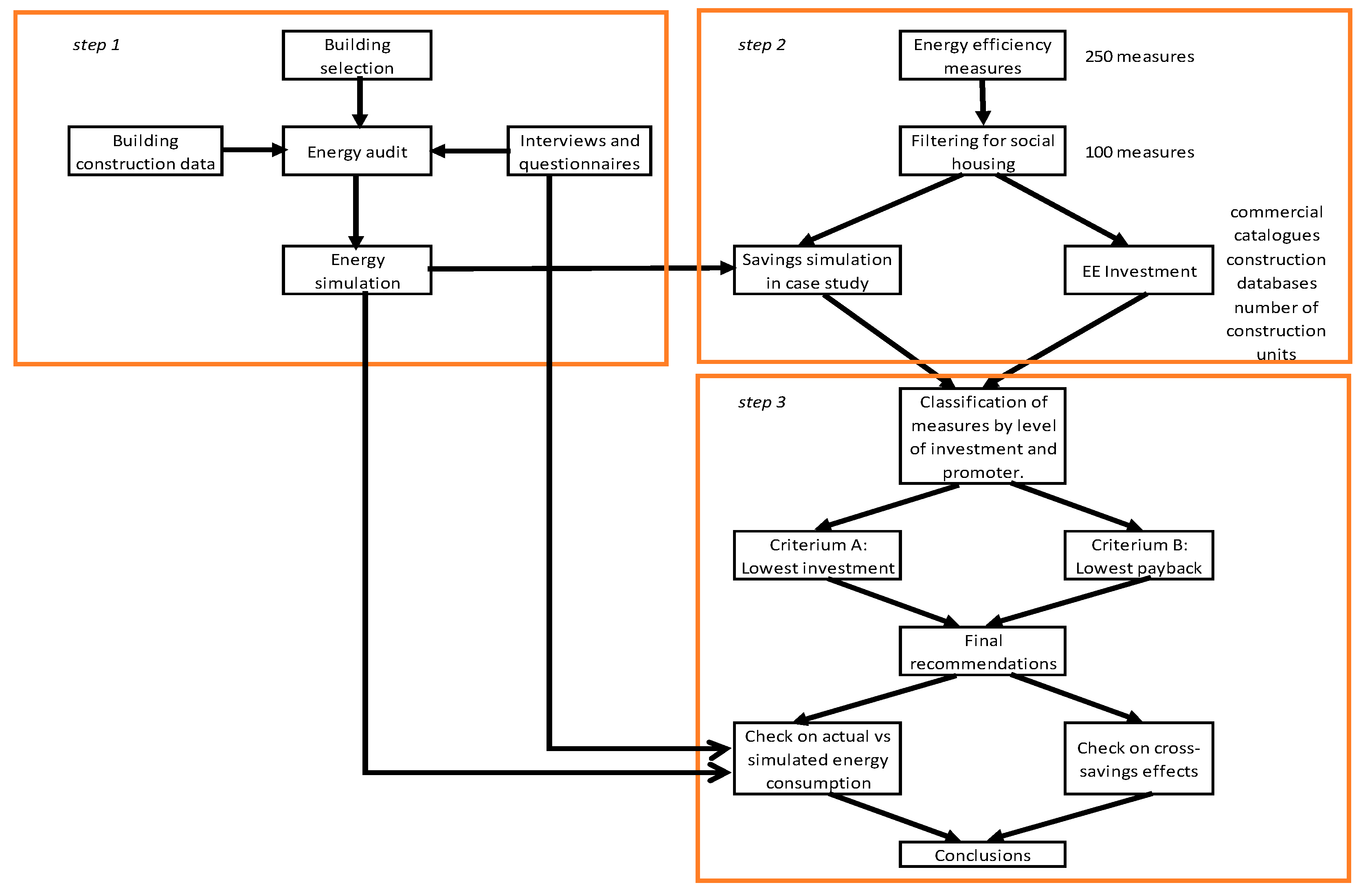
The methodological approach is divided in three steps that eventually converge: on the one side the social housing dwellings for the case study are chosen, characterised and the energy performance evaluated. On the other hand, the energy efficiency measures for buildings are identified, filtered, simulated in the case study building, and evaluated economically. Finally, the energy efficiency measures are prioritized before making the final selection proposal according to different criteria. Final checks and corrections have to be made in terms of real consumption data versus average user profiles based on thermal comfort assumptions, and due to cross saving effects of implementing different measures that affect the same energy consumptions.

In the first step of the methodology, a building with 160 dwellings in the city of Zaragoza (Spain) was selected among a sample of 300 social housing buildings due to the larger number of dwellings and the representability of this type of dwellings in the sample. Two sources of information were sought to gather the necessary data for the energy modelling of the building:

• Construction materials and characteristics of the building, provided by the owner of the building, the municipal company “Zaragoza Vivienda” (Sociedad Municipal “Zaragoza Vivienda”. www.zaragozavivienda.es).
• User profiles gathered from onsite visits and energy bills supplied by a representative sample of 36 dwellings. Comfort temperatures and HVAC schedules were gathered. Three different user profiles were defined under the premise of keeping thermal comfort conditions during the HVAC scheduled hours. These profiles are described in the following epigraph. The annual energy bills of the 36 dwellings were also collected to calculate real consumption average data and correct the simulated results associated to the three user profiles previously defined.

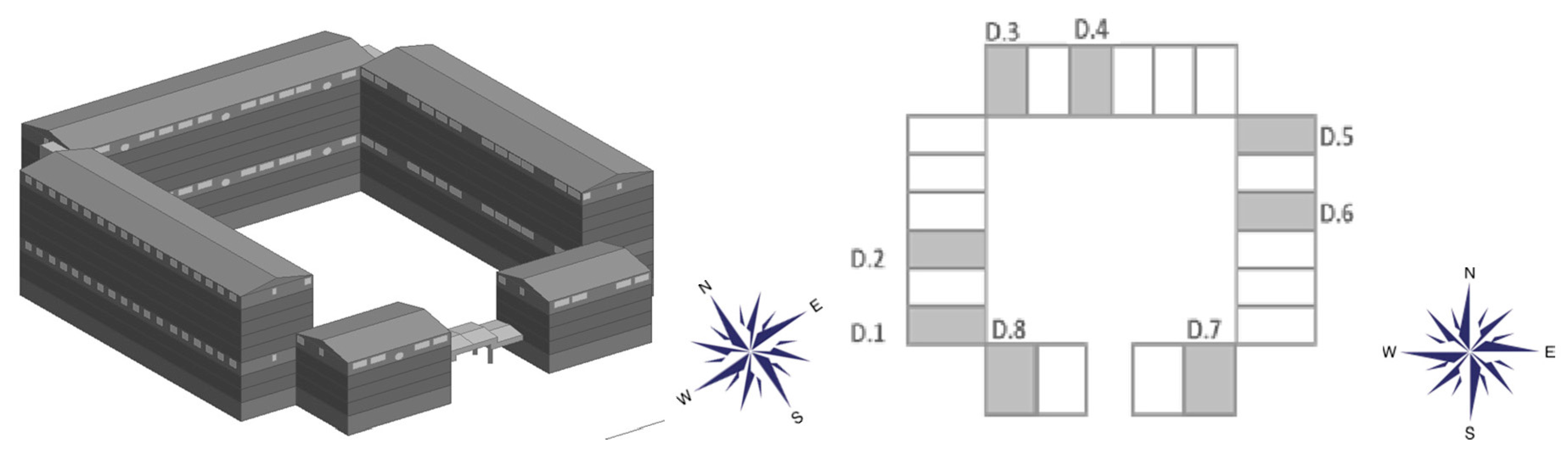
With these values, a building energy performance simulation was done, assessing a yearly thermal demand and an average consumption for eight of the building dwellings using the three user profiles created. The apartments chosen for the simulation were among those visited, and were equally distributed around the four orientations to account for this factor in the energy consumption, as depicted in Figure 1. The representative dwelling of the building is then composed as an average of the eight. In this case, the EnergyPlus calculation engine was used, through the DesignBuilder V4.7 interface [32].

The second step of the methodological approach followed in this paper consisted on the compilation of energy efficiency measures applicable to existing buildings. This was done in the frame of the TRIBE project “TRaIning Behaviours towards Energy efficiency: play it!”, co-funded by the European Union’s 2020 research and innovation programme. In total, 250 energy efficiency measures were identified in all the previous categories and were collected in the TRIBE website [33]. These measures were the result of a holistic energy efficiency assessment in several building types. The different measures were classified according to the energy consumption categories as described below:

• Envelope (E): These are refurbishment measures applicable to the building envelope to reduce the thermal demand, such as adding insulation, thermal bridge breakages, waterproofing, reducing air infiltrations, etc.
• HVAC (H): Heating and ventilation system improvements.
• DHW (D): Domestic Hot Water supply savings and improvements.
• Lighting (L): Indoor lighting savings and improvements.
• Electrical Devices (ED): These measures refer to the better use of more suitable and efficient equipment for home appliances and other common domestic electrical devices. Many behavioural and no cost measures also deal with the efficient use of electrical devices and are contained in this category.
• RES and others (O): Self generation and consumption by means of renewable sources, as well as other type of measures are included.

Measures are codified by using the above designation in brackets, followed by “L” for long term measures or “S” for short term measures, and the correlative number of the action.

Of the total set of 250 measures, only measures applicable to residential blocks of apartments were chosen. In the sample of 300 social housing buildings analysed in this study, no cooling systems were observed in any dwelling. In addition, in the literature review, the existence and use of active cooling systems in this kind of buildings are extremely rare, due to the lower disposable incomes. In these buildings, natural cross ventilation, mainly at night, is the most widely used technique for cooling. Although this is an effective technique it does not usually completely meet the cooling demand, so thermal comfort conditions are not achieved during many summer days. For all these reasons, measures related to cooling systems were dismissed in this study. Similar equivalent measures were also eliminated to avoid redundancy such as the different insulation materials for insulation improvement, or glazing types in the installation of more efficient glazing. Those measures dealing with the design concept of the building were discarded as well as those that were deemed inapplicable in a typical social housing building, ending with a preliminary list of 100 measures.

The third step of the methodology was devoted to assess which energy efficiency measures apply to the case study building. The preliminary measures selected were simulated in the case study using EnergyPlus to obtain annual energy savings, both thermal and electrical for the whole building and per dwelling. Measures were simulated one by one while keeping the rest of the building inputs, user profile and conditions unchanged. Some behavioural measures or many involving recommendations for an efficient use of electrical devices such as kitchen elements could not be simulated in the energy performance software. In this case, savings were taken from other literature sources, averages and manufacturer estimations. Consequently, a significant uncertainty level has to be considered in the assessment of some behavioural measures.

Savings were calculated in kWh/year per dwelling and m², and in €/year per dwelling and m² using an average energy price of 0.045 €/kWh for gas and 0.14 €/kWh for electricity, according to the average tariff provided by the collaborating residents of the building.

An estimation of investment needed was also made using solution providers’ datasheets, commercial catalogues and construction products databases such as BEDEC [34]. A simple payback was calculated for every measure as a ratio of investments versus annual savings in years of investment return, and then compared with the expected lifetime of the implemented action.

The preliminary 100 measures were then distributed by implementation ownership, separating those that correspond to the property of the building (public entity and management service company) and the dwelling tenants. Generally, flats are rented empty with no furniture or user devices that are catered for by the tenants. EE actions related to the building, the external envelope and the HVAC equipment maintenance belongs to the property. This was the situation of the building under analysis. However, this may vary depending on the renting conditions and policies set by the social housing authorities. At each case, the right screening criteria should be applied.

Although not investing in EE also has a cost in terms of extra energy consumed and environmental impacts [35], energy vulnerable families are extremely sensitive to large expenditures, hindering the implementation of many of the above list of measures. They would only undertake no or low investment measures, whereas those involving building equipment and envelope should be promoted by the building property or the management company. Related analysis shows a willingness to pay for energy-saving measures by apartment tenants if the benefit is noticeable [36]. However this may not apply in the case of social housing as low-income tenants who are not home owners are usually less engaged in energy efficiency, as stated by Robison and Jansson-Boyd [37]. Since the level of investment that can be covered by each actor was unknown, they were quizzed about the right level of expenditure per dwelling that each side felt reasonable. Residents claimed that the total aggregated investment should not exceed 500 € in 10 years, whereas the owning property had plans to gradually invest as much as 5000 € per dwelling in a 10 year plan. These were the top budget thresholds proposed for each side.

The next step consisted on an assessment over the most suitable set of practices and measures proposed, based on two different criteria:

• Lowest investment, due to the limited resources available, not only by the apartments’ tenants, but also by the housing managing companies. According to this criterion, EE measures by residents and by property would be taken starting by the lowest cost until the delimited budget is reached.
• Lowest payback, as a ratio of savings provided per economic unit invested. In this case, EE measures would be undertaken starting by the lowest payback until the allocated budget is depleted.

To quantify the optimum budget range for resident and property’s investment in EE, the savings–investment exponential model proposed by Valero [38] was used to determine the maximum achievable accumulative savings derived from the investments and the elasticity of the savings as a function of investment for the set of preliminary measures. The model was developed starting from the characterized EE measures sorted by decreasing payback. Savings were calculated in total value for the whole lifespan of the applied EE measure. The accumulated savings and accumulated investments were then worked out and represented graphically, obtaining the savings–investment curve. Finally, the best fit exponential curve was derived.

S(I) = S_M × (1 − e^−ε*I)

where

• S(I): Accumulated savings for an accumulated investment I, in €/dwelling;
• I: Accumulated investment in €/dwelling;
• S_M: Maximum achievable savings for the total investment I, in €/dwelling; and
• ε: Saturation coefficient of the curve (€⁻¹/dwelling).

The prioritization criteria and the proposed classification is a relevant result of this analysis focusing energy efficiency in social housing. Nevertheless, two important aspects of the results seriously affect the final performance of the building and need a closer look. These aspects were analysed as well:

• Cross-savings of EE measures that are applied simultaneously affecting the same consumption. Total savings of a set of measures have to be simulated together and savings will be lower than the addition of savings, thus increasing the overall payback.
• Real consumptions of the dwellings versus simulated consumptions. Actual energy consumptions turn out to be lower than the simulated energy consumptions. Hence, EE measure implementation bring along lower economic savings than expected, extending the payback period of the investments.

Finally, an extension of the results to the full public Spanish social housing system is done to become aware of the potential of energy sustainability at a national level.

A flow chart of the methodology is depicted in Figure 2.

3. Case Study

A social housing building that represents generic social housing buildings has been chosen to test the different EE measures, recommendations and retrofitting in it. The building chosen for this analysis is situated in the city of Zaragoza (Spain) and is fully dedicated to social housing. This building is being managed by the public company “Zaragoza Vivienda”. This is a square-shape building containing 160 similar dwellings of about 74 m² each in eight floors over ground level.

The case study building was built in 1988 and commissioned in 1990. This is in line with the average age of the social housing building sample, from 1985. It was built with no energy efficiency criteria, under the building regulation in force at the time of construction [22]. It is subjected to a mild Mediterranean dry climate of warm long summers with average temperatures of 25 °C, and short mild winters with average temperatures of 10 °C. The registered annual Heating Degree Days (HDD) using a reference temperature of 15 °C are 1177 HDD, and the annual Cooling Degree Days (CDD) for a reference temperature of 28 °C are 113 CDD (degree days calculated by means of www.degreedays.net). It corresponds to the Spanish climatic zone D3 (“D” indicates the winter weather severity on a scale from A to E and “3” indicates the summer weather severity on a scale from 1 to 4, according to section HE1 in CTE [39]. A1 corresponds to the mildest weather.). The average wind speed is 19 km/h at 20 m high, the predominant wind is cold and dry, in the northwest–southeast direction [40].

There is an important gap for the quality of the envelope with respect to today’s minimum requirements in Spain [39], as shown in

Table 1. Comparison of thermal transmittance of the enclosures of the case study building according to building design values and the value required by current regulations CTE DB-HE1 [39], in W/m²K.

Type of Enclosure	Thermal Transmittance (W/m2K)
	Building Case Study	CTE DB-HE1
External walls	0.71	0.6
Internal walls	2.44	1.2
Bottom floor	1.12	0.4
Roof	0.51	0.4
Windows	5.7	2.7
(glazing type)	(single glass 6 mm)	(-)

. Windows are sliding aluminium frame single glass with thermal bridges showing theoretical transmittances two times larger than today’s construction standards for glazing surfaces. These types of building practices were common at the time of this building construction.

Energy costs are covered by each household with its own resources that may be completed with social bonus and/or other social aids aimed at mitigating energy poverty. In addition, families also pay the social rent, which is a very favourable rate compared with market housing costs and also depends on the family incomes and conditions. For vulnerable households, the main difference between house renting costs and energy costs is that social renting is managed by the local Social Services that may be open to study the situation with the family in case of payment default, whereas the energy supply is managed by private utilities and the failure of payment may result in an energy supply cut [41]. Recently, after RDL 7/2016 [42] and especially in winter time, utilities are not allowed to cut down the energy supply and they must keep the supply while the social services would certify the energy vulnerability [5] and temporarily take up partially or totally the incoming energy invoices.

Apartments have an average occupancy of 3.7 persons per dwelling. They are fitted with individual 24 kW individual gas boilers for DHW and heating and have no cooling systems. The user profile taken corresponds to an average occupancy of three tenants per dwelling, staying at home from 18:00 to 09:00 on weekdays, and all day long on weekends. The average winter set point temperature is 21 °C. Hot water consumption is assumed to be 30 L/day per tenant, with delivery temperature of 55 °C. Heating schedule is from November to March, from 00:00 to 22:00

Table 2. Heating and DHW equipment and user profile.

System	Main Characteristics
Heating	Type of system	Individual atmospheric conventional boiler
	Fuel	Natural gas
	Temperature set point (°C)	21 °C
	Heating capacity (kW)	24 kW
	Heating system seasonal efficiency (%)	72.2%
	Working temperature (°C)	70–80 °C
	Heating distribution network	Monotubular copper installation
	Heating distribution in the dwelling	Steel plate radiator in every room
	Schedule	November to March from 12 a.m. to 10 p.m.
Cooling	No cooling system available in the dwellings
Ventilation	Type	Natural
	Relative humidity set point (%)	40–60%
Domestic Hot Water	Type of system	Same boiler as heating
	Delivery temperature (°C)	55 °C
	Average daily consumption (L/day tenant)	30 L/day per tenant

summarizes the heating and DHW demand data for an average dwelling.

For electrical devices and lighting, three different family profiles have been defined, each one with different occupancy profiles and electrical device use schedules:

• “Working”: Family composed of four members, two adults who work during the weekdays and two children that go to the school. Total lighting hours: 2586 h/year.
• “Part-time”: Family composed of two members who work part time on weekdays. Total lighting hours: 2553 h/year.
• “Not-working”: Family composed of four members, two adults, from which just one of them works on weekdays while the other one is usually at home, and two children that go to school. Total lighting hours: 2804 h/year.

For each of the aforementioned profiles, a specific schedule has been defined for the weekends, which is alternated randomly with other schedule of no occupancy (representing the family leaving the house for the weekend).

4. Results and Discussion

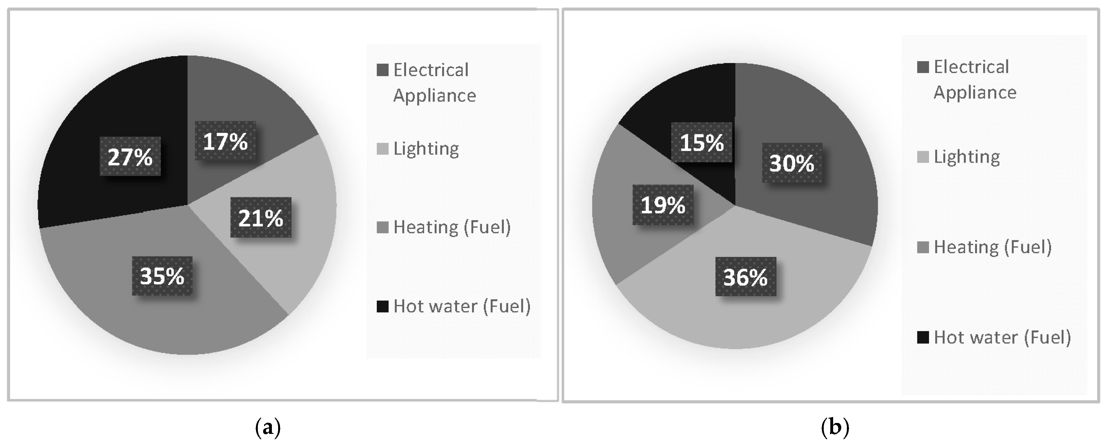
The simulated energy consumption per dwelling and year is 95.8 kWh/m², around 900 €/dwelling, where heating and DHW account for 62% of the annual energy, although they only represent 34% of the energy expenditure (gas consumption) due to the lower natural gas cost with respect to electricity. The large difference of gas and electricity energy costs explains why electricity is two thirds of the total energy costs of these dwellings, as reflected in Figure 3.

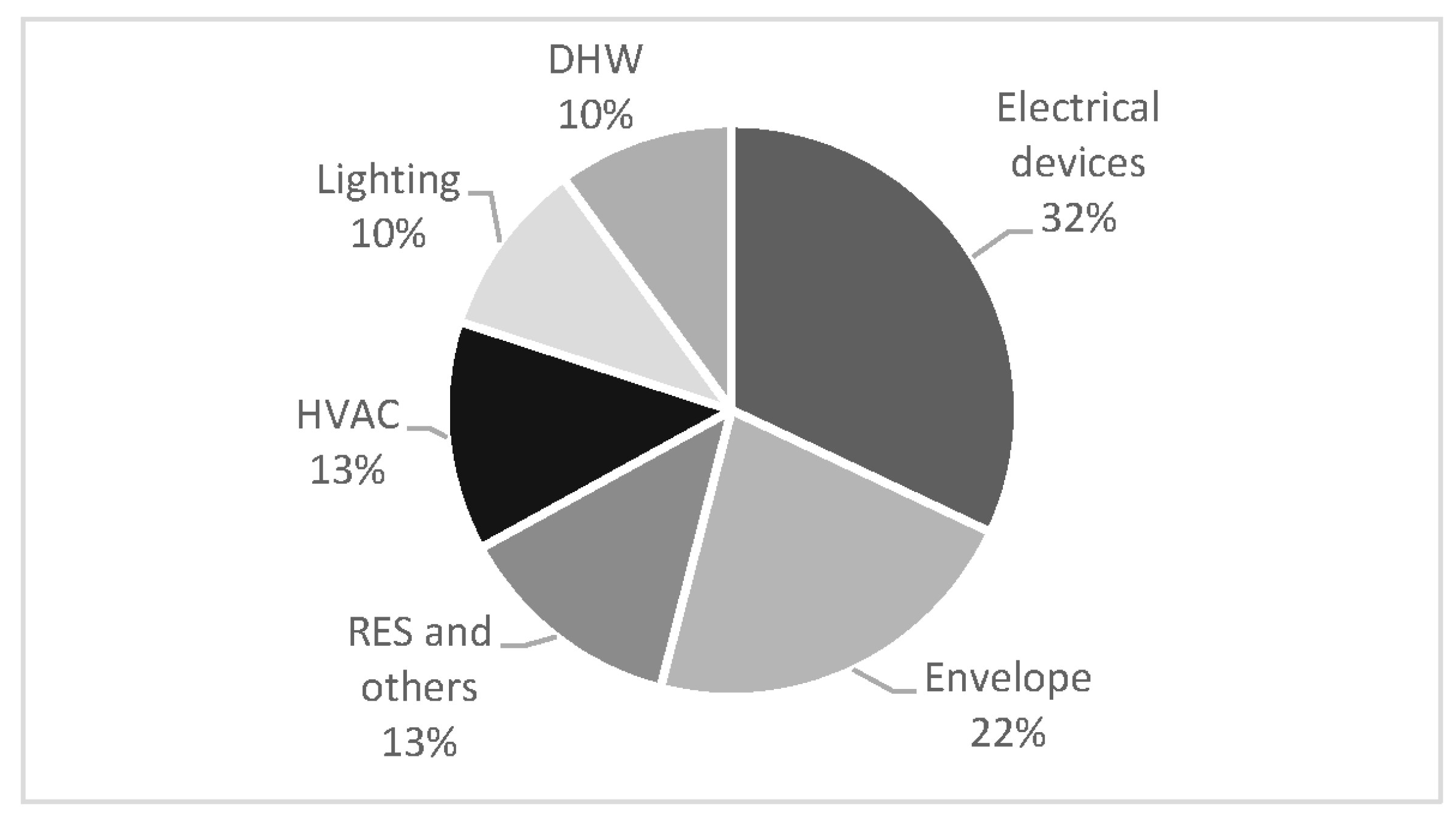
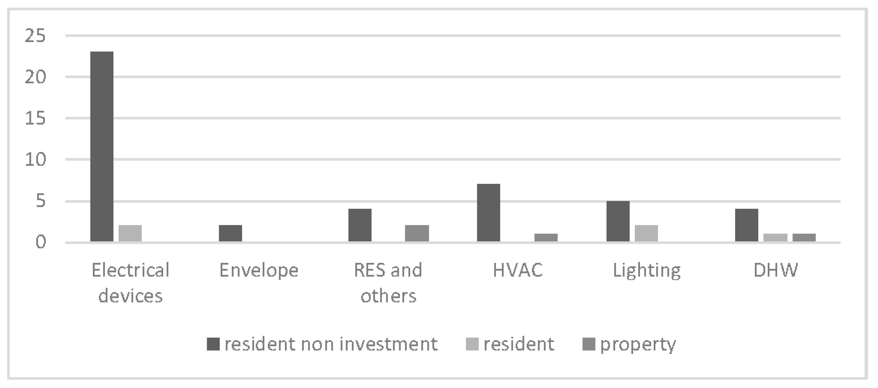
The result of this screening for the applicable 100 EE measures by implementation owner was the following:

• Behavioural change and no investment measures, based on real-time operation of buildings and devices [43], to be implemented by residents: 45 measures.
• Measures requiring investment by the residents: 21 measures.
• Measures requiring investment by the property: 33 measures.

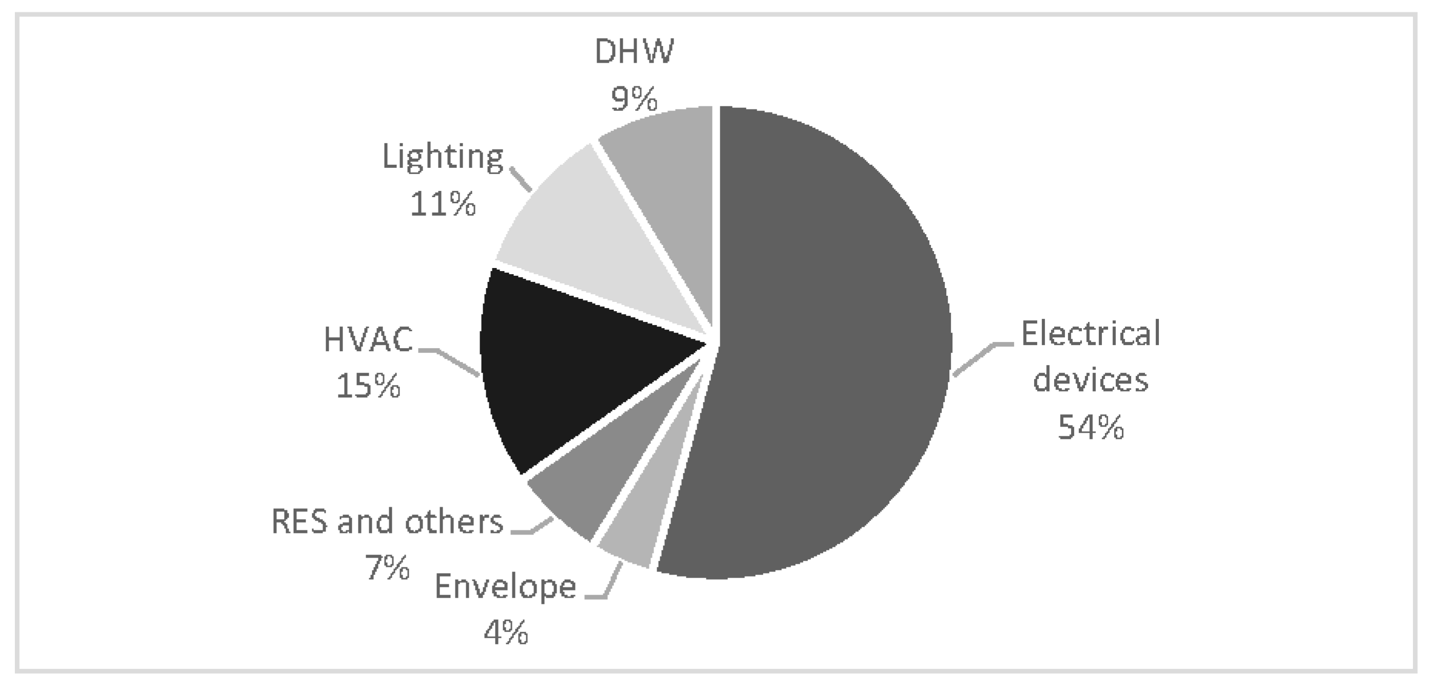
The energy saving categories are evenly distributed with predominance of those involving the optimal use of electrical devices and improvements in the building envelope, according to Figure 4. According to some recent studies, most of the energy efficiency measures implemented in non-profit housing involve the replacement of DHW and HVAC systems [44].

In the case study, envelope, HVAC and DHW measures involve savings in gas consumption as heating and DHW is supplied by means of individual natural gas boilers. Most of the measures in the other categories affect the consumption of electricity.

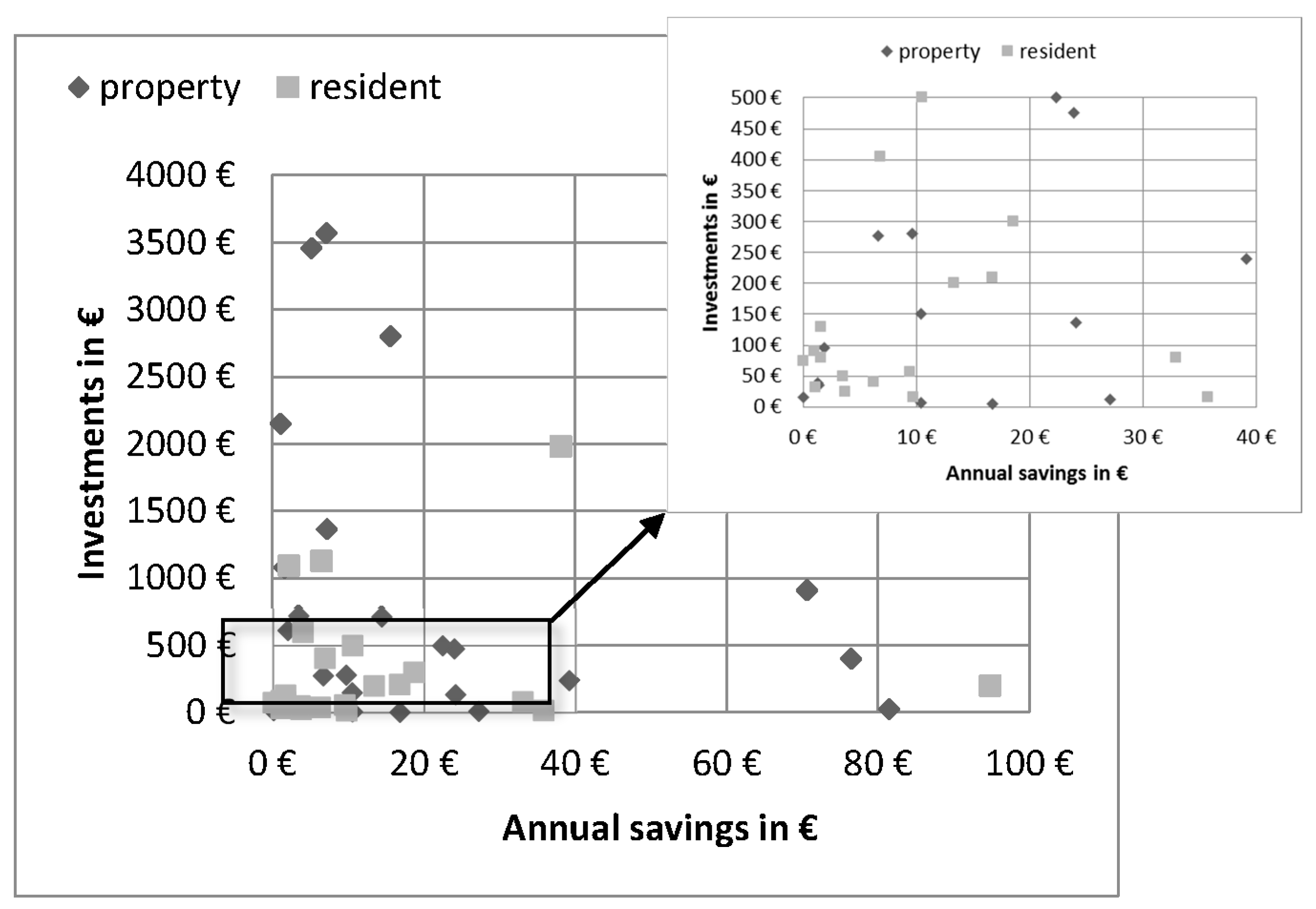
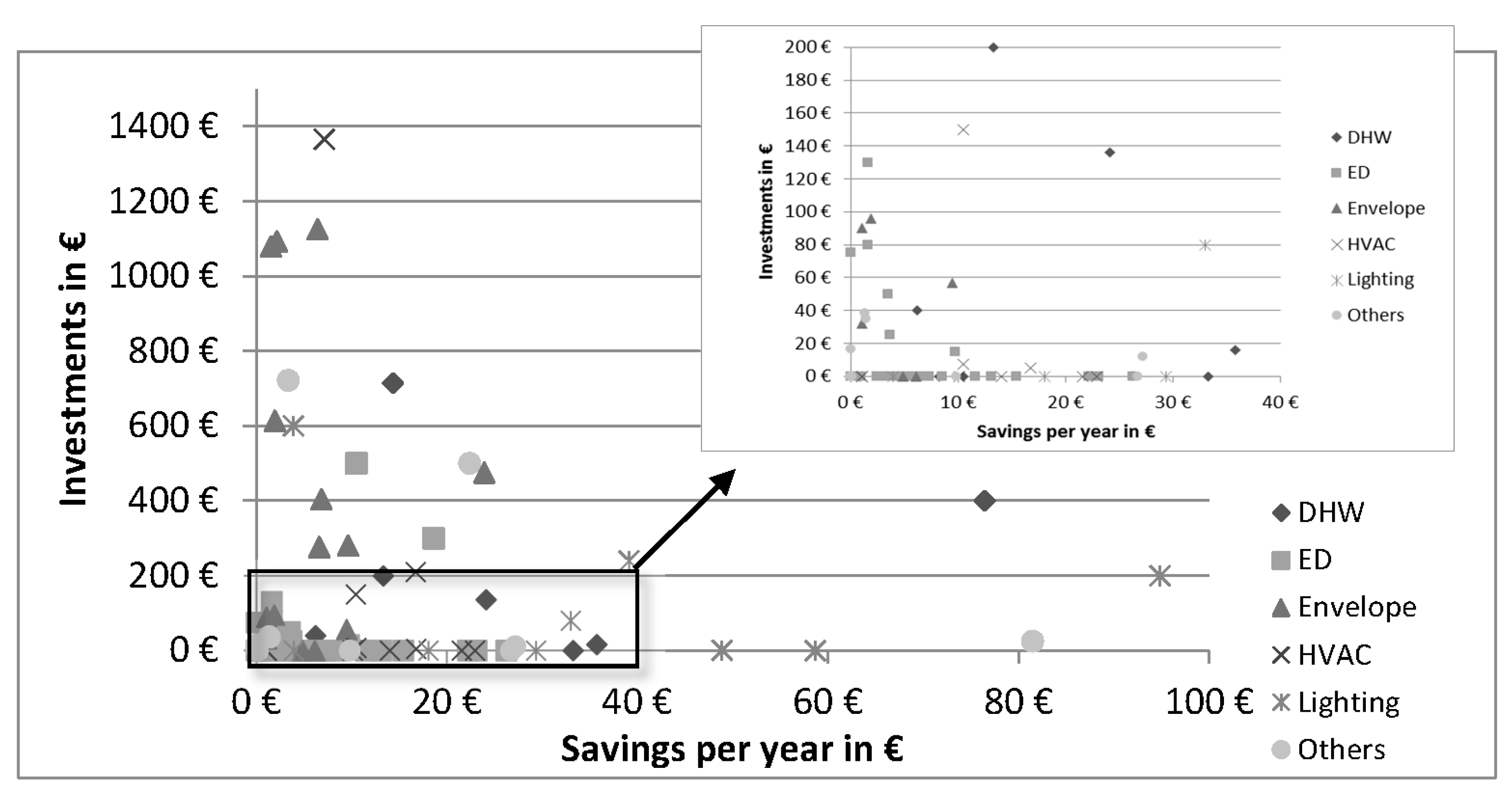
Most measures report savings lower than 50 €/year and require investments lower than 1000 €. This is mainly the case for the EE measures attributed to the residents. Non-investment EE measures have been removed from Figure 5.

Regarding measure category, envelope-concerning measures require the highest investments with modest savings, whereas lighting measures involve the lowest investment for acceptable savings. Many electrical devices measures mean no investment as depicted in Figure 6.

4.1. Prioritization Criteria for EE Actions

The results show that two thirds of the measures lay on the tenants’ responsibility. In a context of social housing, residents are likely to be very sensitive to large investment expenditures to undertake many of the proposed EE actions. Hence, a prioritization criterion should be the necessary level of investment to implement each measure, starting by those measures that require no investment or just entail a user behavioural change and followed by the fastest and lowest price measures in order to allow for the maximum number of EE measures to be implemented with a limited budget. This budget is the maximum amount of money that the implementing owners are willing to spend on EE in a given time. This question was posed to the residents and to the property for a period of 10 years and the average answer by the 36 questioned flat tenants was around 500 € and for the building management company (property) 5000 €/dwelling.

Most of the EE measure’s lifespan are above 10 years with a mean of 16 years. Only measures related to annual maintenance have shorter lifespan, often just one year.

To obtain the fastest results at no cost, the behavioural and no investment measures should be prioritized. Almost half of the measures are within this category. They are grouped by type of measure in

Table 3. List of zero investment and user behavioural measures grouped by type of measure and sorted by annual savings in aggregated €/dwelling.

Type of Measure	Number of Measures	Savings per Year
		Energy Saving (%)	Cost Saving (€/Dwelling)
Electrical devices	25	22%	186 €
Lighting	5	17%	159 €
HVAC	6	23%	71 €
Others	5	11%	65 €
DHW	4	17%	53 €

, and then sorted by decreasing annual expected savings. The percentage of savings is calculated with respect to the total simulated dwelling energy consumption per year in kWh.

These EE measures, in general, cover all possible categories of energy efficiency, but more than half refer to the optimal usage of electrical devices usually available in residential households, as shown in Figure 7. These measures are easy to implement and involve almost no investment but their implementation is rather unpredictable, since their success is based on the residents’ knowledge and skills, habits, technology used, awareness and their willingness to collaborate [45], despite the fact that they are the greater beneficiaries of the savings achieved. The measures individually contribute little to the overall energy consumption reduction, but due to the immediate results and the need of no investment, they should be the first to be implemented to obtain fast savings to mitigate extreme energy poverty cases.

To achieve further savings, some investments should be made, either by the residents or by the building property. At this point, a question arises about the criteria to prioritise the implementation of EE measures. The usual criteria is the economic simple payback since this metric ensures the maximum return in savings for a given investment and hence, the inclusion of the best EE investments. However, given the low economic resources of the residents of this type of building, and to ensure a higher number of EE measures for a given budget, it is proposed to consider the advantages of using the lowest investment as a criteria to sort out EE measures.

With this latest criteria, on the side of the residents, the 500 € budget would give room for 10 EE measures obtaining a total saving of 104 €/year per dwelling, no cross-effect considered. The list of low investment EE measures to be implemented by the residents is shown in

Table 4. List of resident low investment EE measures sorted by lowest investment per dwelling.

Code	EE Measure Description	Energy Saving (%)	Payback (Years)	Lifespan (Years)
EDS35	Decalcify home appliances	1%	1.5	1
DS8	Installation of taps with flow reduction (faucet aerator)	11.8%	0.4	15
EDS1	Use of multiple power strips with switch and/or programmable plugs	0.4%	6.8	10
ES9	Substitution of roller tape guide	0.3%	30.6	30
DS10	Installation of low-flow showerheads	2.1%	6.5	10
EDS24	Repair refrigerator door seals	0.4%	14.3	10
ES1	Use silicone, putty or draught excluder to reduce air infiltrations through windows and doors	3.1%	6	10
EDS30	Promote the use of solar chargers	0%	9403	2
LL2	Installation of electronic ballast	3.5%	2.4	15
EDS16	Use a toaster oven or microwave instead of the oven	0.2%	50	5

.

EE measures being rejected by this sorting criteria relate to the purchase of expensive more efficient equipment and appliances. However, it can be observed that some of the prioritised measures have longer estimated payback than lifespan.

On the side of the property, there are 19 EE measures within a limited budget of 5000 €/dwelling. The total accumulated savings sum up 373 €/year per dwelling, no cross-effect considered. They are shown in

Table 5. List of property low investment EE measures sorted by lowest investment per dwelling.

Code	EE Measure Description	Energy Saving (%)	Payback (Years)	Lifespan (Years)
HS9	Adding or repairing boilers insulation	6%	0.3	15
HS7	Analysis of the combustion and maintenance of heating boilers	3%	0.7	1
OS4	Sensitizing of occupants through workshops	5%	0.4	-
OS3	Inspection and maintenance of lifts	0%	465.3	1
OS7	Create reminders and promotional materials to raise awareness	15%	0.3	2
OL6	Installation of an ICT system	0%	25.2	20
OL5	Installation of a Building Energy Management System (BEMS)	0%	29.1	20
ES10	Maintenance of wood and aluminium windows frame	1%	51.5	1
DS3	Adding or repairing DHW distribution systems	8%	5.7	15
HS24	Installation of thermostatic radiator valves	3%	14.4	20
LL11	Installation of manual potentiometric switches	4%	6.1	10
EL29	Application of an appropriate solar reflectance coating for the external walls	2%	41.9	10
EL26	Improve insulation in thermal bridge areas	3%	29.2	30
DL6	Installation of Drain Water Heat Recovery (DWHR) systems	25%	5.2	30
ES2	Seal air leaks located in all cavities presented in the building	8%	19.9	15
OL7	Installation of smart meters	2%	22.3	15
EL6	Adding or increasing internal insulation in roofs	1%	319.8	30
DL5	Change from an individual to a collective DHW system	5%	49.8	30
OL3	Installation of direct traction electric lifts	0.4%	216	15

where, again, payback periods exceed solution life expectancy in many cases.

Actions out of budget include efficient window replacement, envelope insulation improvement, efficient low temperature heating equipment, ventilated façade and other high-cost measures.

When applying the traditional payback criterion, results change significantly in some cases. For the resident side, the number of measures under budget goes down from 10 to 7 but increasing the savings per year from 104 €/dwelling to 193 €/dwelling. The new list of EE measures by decreasing payback is represented in

Table 6. List of resident low investment EE measures sorted by lowest payback in years.

Code	EE Measure Description	Energy Saving (%)	Payback (Years)	Lifespan (Years)
DS8	Installation of taps with flow reduction (faucet aerator)	11.8%	0.4	15
EDS35	Decalcify home appliances	1%	1.5	1
LL4	Replacement of incandescent lamps by Compact fluorescent lamps (CFLs)	10.2%	2.1	15
LL2	Installation of electronic ballast	3.5%	2.4	15
ES1	Use silicone, putty or draught excluder to reduce air infiltrations through windows and doors	3.1%	6	10
DS10	Installation of low-flow showerheads	2.1%	6.5	10
EDS1	Use of multiple power strips with switch and/or programmable plugs	0.4%	6.8	10

. The only difference when compared with Table 4 is LL4, replacing incandescent lamps by fluorescent lamps, with a high investment but providing significant savings, and with better payback than LED lighting replacement (not selected due to redundancy). In all cases, the payback in years is shorter than the expected measure lifespan. In this case, no measure’s estimated payback exceeds the expected lifespan.

In the case of the property low investment measures, the new list sorted by lowest payback and meeting the maximum affordable budget goes down from 19 to 10 EE measures, but the amount of accumulated annual savings increases by 38% from 373 €/dwelling to 605 €/dwelling (

Table 7. List of property low investment EE measures sorted by lowest payback in years.

Code	EE Measure Description	Energy Saving (%)	Payback (Years)	Lifespan (Years)
OS7	Create reminders and promotional materials to raise awareness	15%	0.3	2
OS4	Sensitizing of occupants through workshops	5%	0.4	-
HS7	Analysis of the combustion and maintenance of heating boilers	3.5%	0.7	1
DL6	Installation of Drain Water Heat Recovery (DWHR) systems	25.3%	5.2	30
DS3	Adding or repairing DHW distribution systems	8%	5.7	15
LL11	Installation of manual potentiometric switches	4.2%	6.1	10
OL2	Installation of photovoltaic panels	25.9%	10.5	20
OL1	Installation of solar thermal panels for DHW	23.3%	12.9	20
HS24	Installation of thermostatic radiator valves	3.4%	14.4	20
ES2	Seal air leaks located in all cavities presented in the building (Rejected)	7.9%	19.9	15

). The main difference is the inclusion of measures OL1 and OL2 dealing with the installation of renewable solar sources that bring in very interesting savings despite the high installation cost. An important check to be done is that all measures’ estimated payback stays below the expected lifespan. It is not the case for the last measure, about sealing air leaks, whose payback (20 years) exceeds the estimated lifespan of the investment (15 years). This measure should be deleted from the list or replaced by the following in the list. However, the rest of the analysed measures’ payback turns out to be longer than the estimated lifespan. Hence, the recommendation is to stop the measure deployment at this point, resulting in a total property investment of 4424 €/dwelling and total annual savings of 581 €/dwelling, which means an overall payback of 7.6 years. The kind of actions under the property’s responsibility can be easily deployed by means of an ESCO business model as illustrated by Yi et al. [46].

On the other hand, measure OS4, sensitizing occupants through workshops, is a necessary measure to enable the resident’s awareness and involvement in the energy vulnerability mitigation [47]. This measure is to be promoted by the management entity, which, in the case of public social housing in Spain, is the property of the buildings.

In other words, although most of the EE measures recommended match both sorting criteria, the payback sorting option is best as the resulting measures are more optimal and enable larger energy and economic savings.

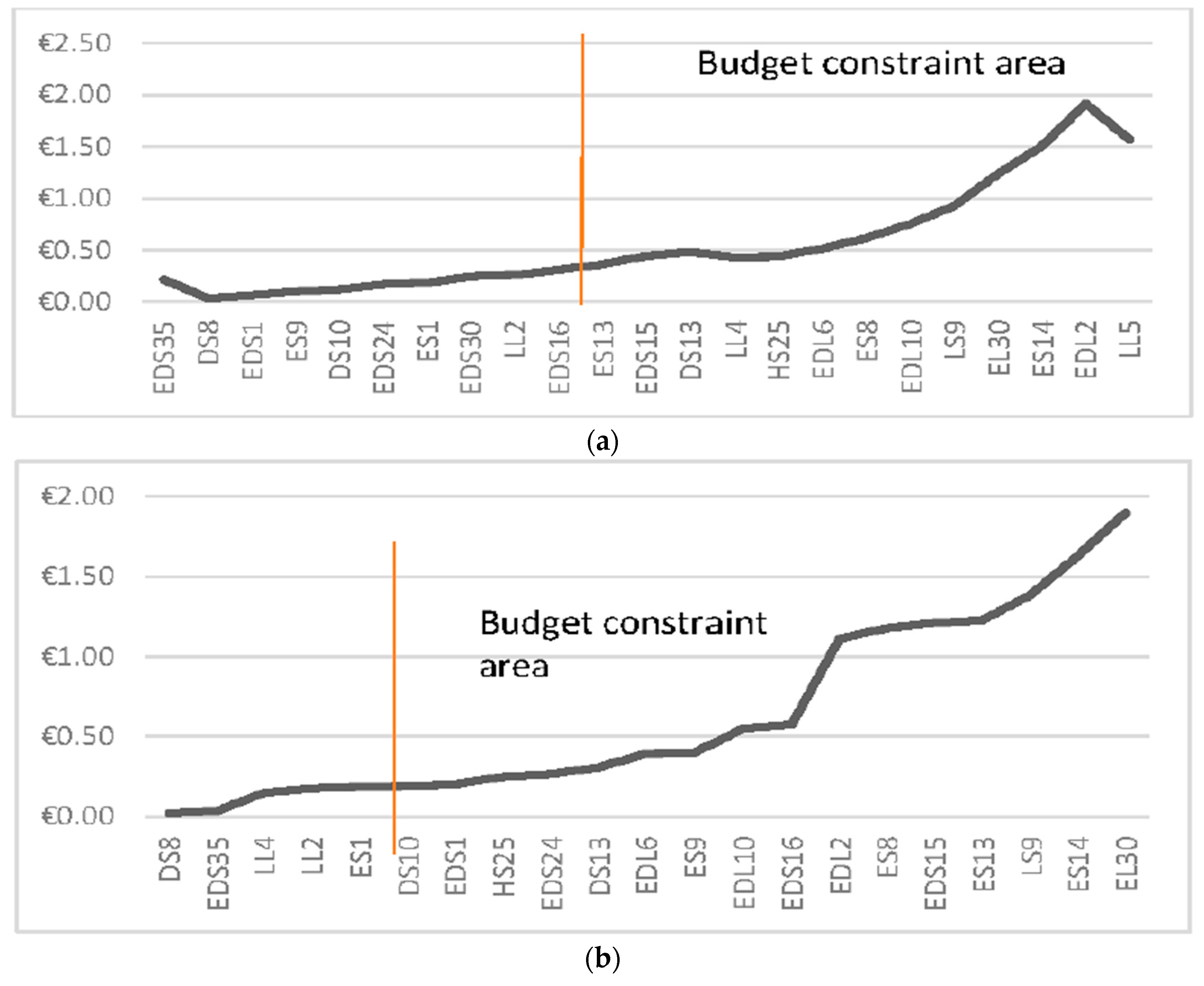
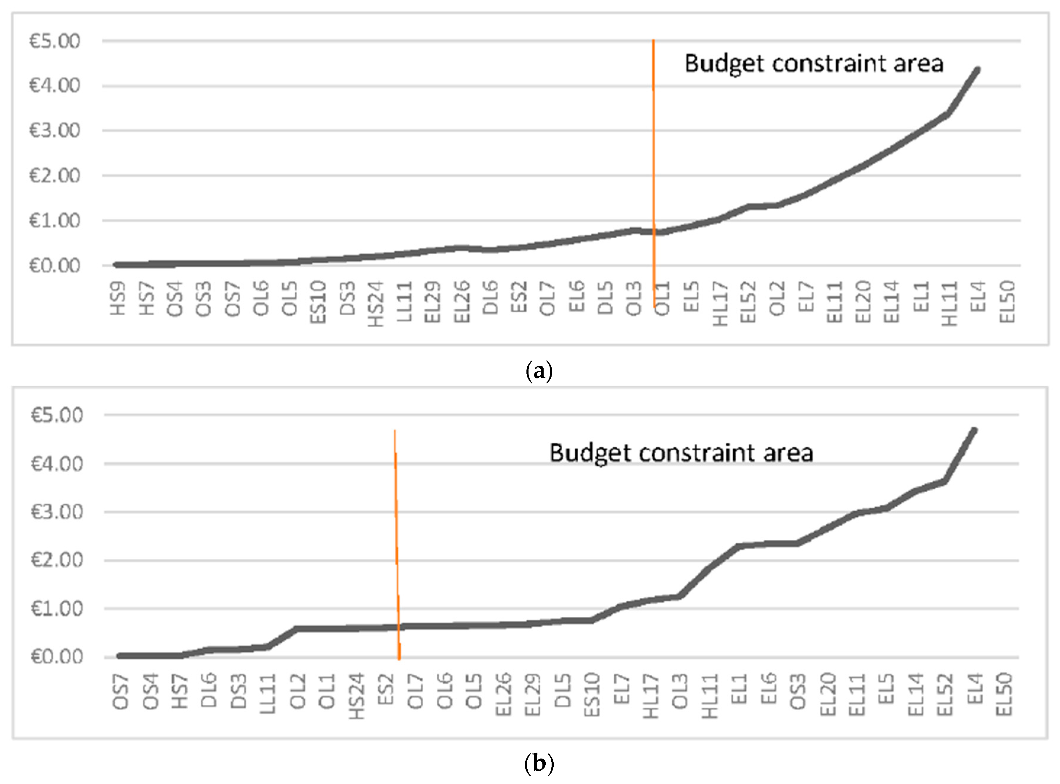
Looking at the cost per kWh saved per year in an average dwelling, as can be seen in Figure 8, the cost of the marginal EE measure meeting the resident budget constraints is 0.3 €/kWh saved following the lowest investment criterion, and 0.2 €/kWh by the lowest payback.

For property owned EE measures, the marginal EE measure shows a cost of 0.77 €/kWh of annual savings if sorted by lowest investment. This cost goes down to 0.61 €/kWh if sorted by payback (Figure 9). In both cases, the best results are obtained by the lowest payback sorting option.

4.2. Sorting Model Based on Savings–Investment Curves

The sorting methodology is independent of the budget constraints, but, in the case there was no budget restrictions, a question that remains is what the most appropriate budget would be to invest in energy efficiency, as the higher the budget the more EE measures that can be implemented but the lower the payback of the additional investments. A suitable way to deal with this issue is by using the savings–investment exponential model proposed by Valero [38].

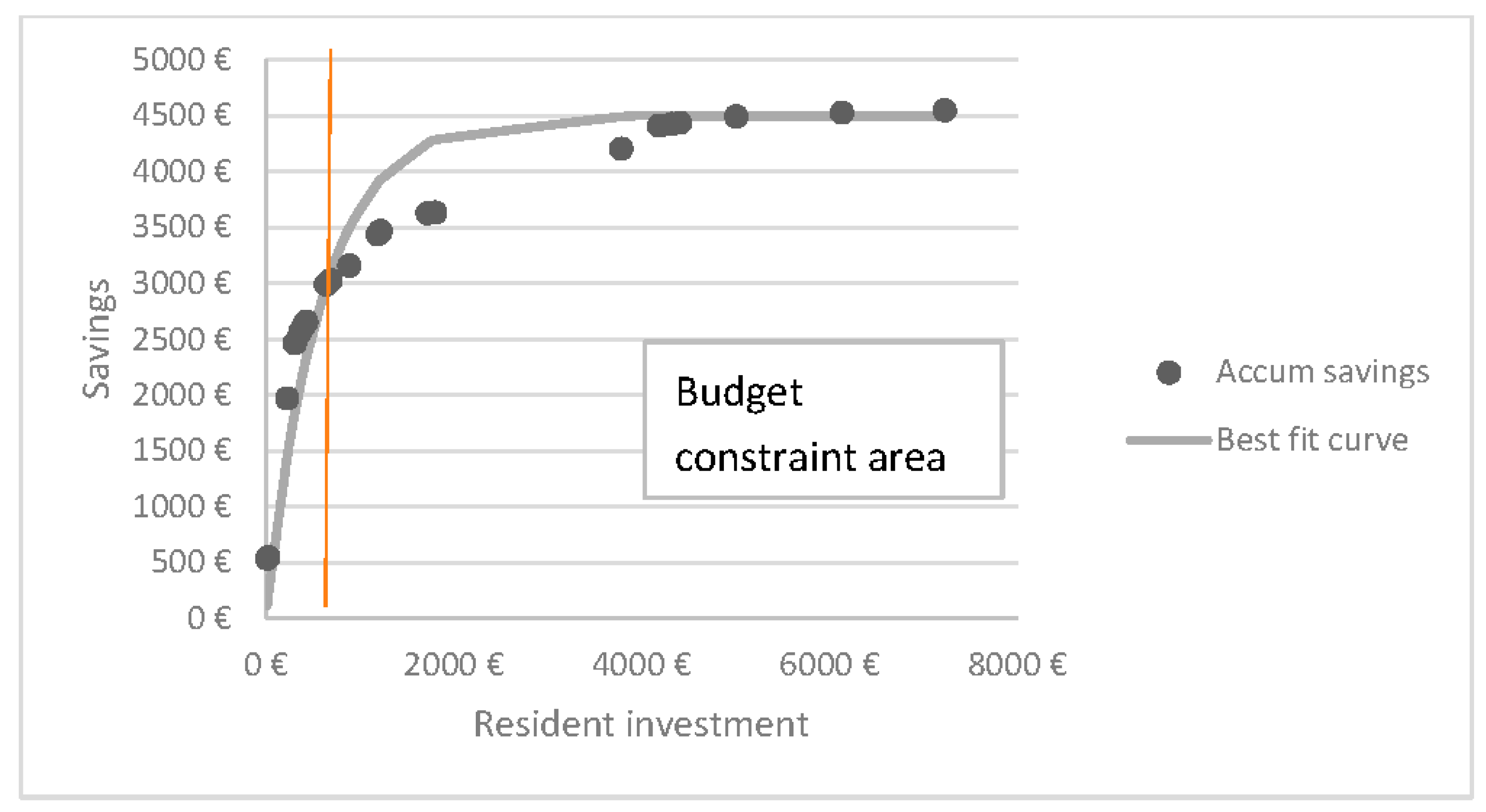
Looking first at the resident EE measures that imply a level of investment, the maximum achievable saving is around 4500 €/dwelling and the saturation coefficient ε = −0.0017 €⁻¹/dwelling. It can be seen that from 1800 €/dwelling of accumulated investment there is no significant improvement in savings. The budget restriction in this case is placed far below, at 500 €/dwelling, the investment saturating level of 1800 €/dwelling (Figure 10). Above this threshold, an increase in investment brings along decreasing absolute savings.

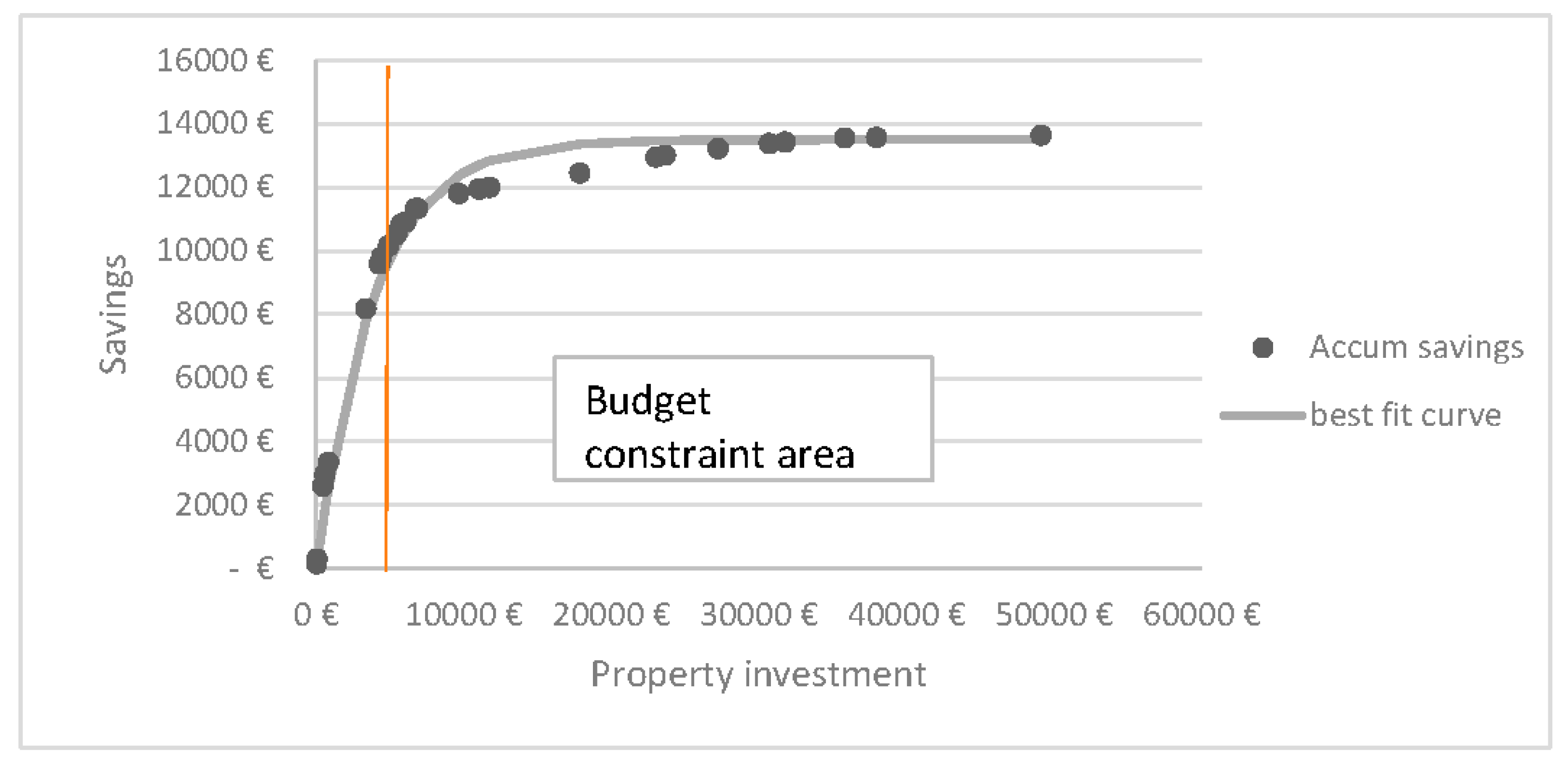
Doing the same exercise for property owned EE measures, the savings–investment curve in Figure 11 shows a maximum achievable accumulated saving of nearly 14,000 €/dwelling, and a saturation coefficient of ε = −0.00026 €⁻¹. The elasticity grade in this case is lower and the savings–investment curve saturates at an optimum investment level of 9600 €. Again, the level of 5000 € is appropriate, as it is below this saturating investment level.

4.3. Simulated versus Real Energy Savings

In total, the 100 EE measures for this social housing building are distributed in 45 behavioural change recommendations, seven low investment measures to be done by the residents and nine by the property, while 39 are rejected for budget constraints or larger payback than lifespan (Figure 12). This distribution shows that 68% of the applicable measures and 84% of the selected measures are under the tenants’ responsibility, becoming the key players to drive consumption down. To ensure that all households are in the position of taking active action towards energy efficiency, programmes offering modest economic aids or loans to be paid back by means of energy savings could be of great help.

The calculations done so far are all based on energy simulations on an average dwelling. Nevertheless, the actual consumption may differ from the simulated consumption. Therefore, some corrections need to be done to obtain more realistic saving forecasts from the implementation of the selected EE measures and calculate the real payback of the investments.

Real consumption data from actual utility billing were collected and a weighted average in terms of dwelling size and orientation was estimated to compare with the simulated consumption of the average dwelling. Results per type of energy and dwelling can be seen in

Table 8. Difference of energy consumption for simulated and real consumption in kWh/year per dwelling.

Type of Energy	Simulated Energy Consumption (kWh/Year)	Real Energy Consumption (kWh/Year)	Difference (%)
Electricity	2669	2056	23%
Gas	5699	3947	31%
Total	8368	6003	28%

.

The real energy consumption is about 30% lower than the simulated energy, and will presumably have an effect on the expected savings, as already identified in some studies such as Teli et al. [48]. This gap between simulated and actual consumption is due to several factors:

• Degradation of the materials and building with time: The simulation has been done with project data thermal transmittances that may have changed along time. The lack of insulation in the building and the good maintenance may diminish this factor. The measurements taken on the walls of the building analysed showed little change with respect to the theoretical values of Table 1.
• Climatic differences of the database reference year (2002) and the billing year (2015): This difference is 1.1 °C colder in winter 2015 with respect to 2002, which should have increased the actual consumption by 7.7%. This factor though, has been corrected by using 2015 heating degree days (1147 HDD) and the same seasonal temperature profile of year 2002, according to the simulation software features [32].
• Level of occupation of dwellings: Although this should be a relevant factor, looking at the annual energy expenditure per household with respect to occupancy, there are no trend lines. Only single-occupant dwellings may show some differences in consumption, but the number of apartments in this situation is just 11% of the sample.
• Lower usage of heating, DHW and electric devices than an average resident, due to the issue of energy poverty in the building, as corroborated by Teres-Zubiaga et al. [49]: The lack of economic resources and the fear of a power cut in the case of non-payment force many of these families to sacrifice thermal comfort, either by setting lower target indoor temperatures or reducing the number of heating hours. This is, in fact, a true issue in social housing and the error versus standard comfort temperatures considered in the simulated user profiles may be significant. This factor does not only affect thermal comfort in social housing but it could have serious impacts on tenants’ health as exposed by Maqbool et al. [50]. The simulated user profiles based on the tenants’ habits information and the real usage models can deviate to some extent, as reported by Silva et al. [51] and Herrando et al. [52].

This last factor jeopardizes the calculated savings of the different EE measures that will be around 30% lower than initially calculated, affecting the payback in the same way. Electricity saving measures become more interesting as the correction factor is lower (23% vs. 31%) but especially due to the much higher cost of the electricity with respect to gas. The high cost of electricity in many European countries is a serious issue for energy poverty since many social housing buildings in Southern Europe run only on electricity, aggravating the problem of energy affordability for many economically vulnerable households.

Applying the actual average consumption correction factors for gas and electricity, the real savings obtained decrease for each measure versus the calculated saving, as represented in

Table 9. Summary of savings including the correction of the actual social housing annual energy consumption.

Type of Measure	Number of Measures	Investment (€/Dwelling)	Calculated Annual Savings (€/Dwelling)	Calculated Payback (Years)	Real Annual Savings (€/Dwelling)	Real Payback (Years)
Resident no investment	45	-	534 €	-	410 €	-
Resident low investment	7	433 €	193 €	2.2	144 €	3
Property low investment	9	4424 €	581 €	7.6	449 €	9.8
Total	61	4857 €	1308 €	3.7	1003 €	4.8

. Total savings achieved in the case of the implementation of the 61 EE measures go down about 30% ending in 1000 €/dwelling per year. The total payback time increases one year to almost five years for the full set of measures.

The second correcting factor for the energy saving estimations is the saving cross-effect of several EE measures implemented together and affecting the same demand. This is specially the case of gas savings as they involve only heating and DHW. Acting on envelope and on boiler equipment simultaneously maximizes the absolute savings achieved by the combination of both measures together but their individual saving contribution of each measure cannot be added to each as the investments do. Hence, the payback of the joint measures increases.

However, some EE measures have additional impacts on savings (such as using microwave instead of oven, decalcifying home appliances or switching off unused equipment). These measures represent independent savings and do not interfere with other measures. The sequence in which they are implemented does not affect the final savings. Usually measures with additional impacts are behavioural and imply electrical savings when using home appliances efficiently. A total of 31 EE measures can be classified as providing additional savings.

The remaining EE measures show cross-effects to some extent. Savings achieved by the previously deployed measures on a given demand (lighting, HVAC, and DHW) will diminish the capacity of obtaining the expected savings of a cross-effect measure as it acts on declining consumptions.

EE measures have been classified by providing additional or cross-effect savings and by the demand they serve (lighting, heating, DHW and others) and, in the case of the latest, the expected savings have been calculated on the decreasing demand, giving the results shown in

Table 10. Summary of savings including the correction of the cross-effect annual energy savings.

Type of Measure	Number of Measures with Additional Savings	Number of Measures with Cross-Effect Savings	Investment (€/Dwelling)	Real Annual Savings (€/Dwelling)	Corrected Annual Savings (€/Dwelling)	Corrected Payback (Years)
Resident no investment	29	16	-	410 €	352.8 €	-
Resident low investment	2	5	433 €	144 €	97.4 €	4.4
Property low investment	0	9	4424 €	449 €	153.6 €	28.8
Total	31	30	4857 €	1003 €	604 €	8

. For this calculation, it has been assumed that measures have been implemented in declining payback order, starting by the no investment measures, followed by the resident low investment measures and finishing with the property investment measures.

The final payback period is up to eight years, which is still acceptable for investments in the residential sector. However, the convenience of implementation has to be checked again on a one to one basis, calculating the new paybacks and comparing them with the expected lifetime of each measure. Measures ES1 and DS10 now do not comply with the payback criteria and should be turned down, leaving the list with just 5 measures (DS8, EDS35, LL4, LL2 and EDS1) and a total investment lower than 400 € per dwelling and a total annual saving of 92.3 €/dwelling, with a payback of just 4.3 years.

In the case of the property low investment measures, there are more that do not comply with the payback criteria, limiting the applicable list to four measures (OS7, OS4, HS7 and DL6).

The summary savings are given in

Table 11. Summary of savings of the selected measures to be applied by residents and property and corrected by real consumption and cross-effect savings.

Type of Measure	Number of Measures	Investment (€/Dwelling)	Corrected Annual Savings (€/Dwelling)	Corrected Payback (Years)	Energy Savings (%)
Resident no investment	45	-	353 €		38%
Resident low investment	5	336 €	92.3 €	3.6	10%
Property low investment	4	444 €	64.5 €	6.9	7%
Total	54	780 €	510 €	1.5	55%

, where 55% of savings with respect to initial energy costs have been achieved at very low cost (780 €/dwelling), shared by the beneficiary resident (336 €/dwelling) and the property (444 €/dwelling). The list of EE measures to implement may be incremented if some of the selected measures, especially those pertaining to behavioural aspects, do not apply in some cases or are already implemented. This way, new low cost measures in the list may become applicable. On the other hand, many of these energy savings might not translate into economical savings but into further margin to increase consumption for the same energy cost, in an attempt to improve the thermal comfort of these energy vulnerable households and enhance their life standards.

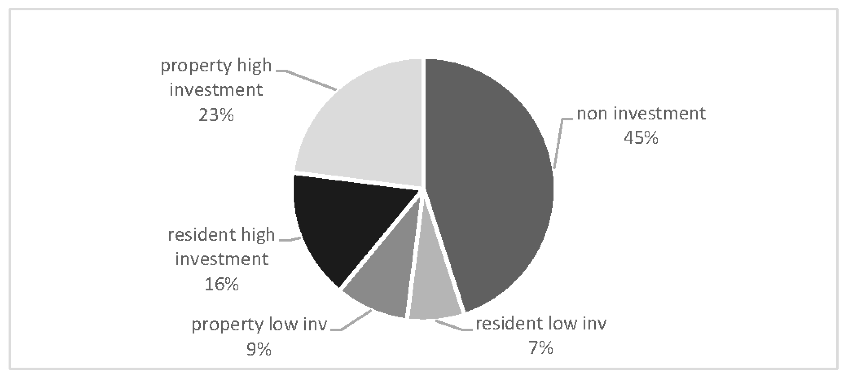
Seventy per cent of the selected measures involve electricity savings as a consequence of the faster return of a more expensive energy source. On the other hand, only 7% of the selected measures are under the property responsibility, making the beneficiary of the measures the main actor in energy savings. The distribution of measures per saving category shows that nearly half of the measures deal with the efficient use and selection of electrical devices, while envelope improvement measures look less attractive for investment (Figure 13).

5. Conclusions

Building refurbishment is a secure investment to minimise the problem of recurrent energy poverty in households. Energy savings can contribute to both reducing the energy cost burden for vulnerable consumers and increasing their level of thermal comfort. However, due to the dwelling tenancy system, a collaborative measure implementation plan between residents and building owner or manager has to be designed, to avoid redundant measures and maximise the result of the combined investment.

When selecting the best energy efficiency options from a list of opportunities, the characteristics of the residential buildings and the typology of vulnerable households have to be considered. About 100 EE measures have been found applicable in a representative social housing building in Spain, and 64 of them have no investment or lower than 100 € per dwelling.

It is recommended to start by the non-investment measures, since the return on these measures is immediate in time. For these measures, the prioritization criterion should be the increasing amount of energy savings expected.

For the necessary investments, a budget threshold is necessary to share the investments between the beneficiary tenants and the property. Residents of social housing are often affected by energy vulnerability and their investment capacity is usually low. However, 70% of the EE measures lay on their side. Hence, their involvement and commitment is crucial.

To make sure that the budget threshold is correctly set, the savings–investment exponential curves can be used to calculate the maximum savings attainable by the implementation of sequential investments in energy efficiency. These curves also help to determine the limit at which further investment do not significantly contribute to get extra energy savings.

The sorting criterion based on lowest payback yields better saving results for the same investment budget than it does the sorting by lowest investment. The aggregated annual saving for non-investment measures is 534 €/dwelling while the aggregated annual savings of measures within budget limits is 774 €/dwelling with a simple payback of 6.3 years. When correcting with actual consumptions, savings get reduced to 410 €/dwelling for non-investment measures, and 593 €/dwelling with a payback of 8.2 years.

Energy simulation tools have proven to be affordable, fast and convenient to assess the energy saving potential of each measure implemented in a building. However, the real saving values are usually 20–30% lower than the simulated results, mainly because simulated demand is calculated to meet standard thermal comfort conditions which are not always met in this type of housing due to their economic limitations. Furthermore, the cross-effect of the simultaneous implementation of energy efficiency savings addressing the same energy saving category is significant and should be taken into account when assessing payback periods.

The results of the study prove that, with minimum investment levels, shared by flat tenants and building property, a considerable amount of savings can be obtained (up to 55% of the initial energy consumption). The deployment priority to be followed is first the non-investment measures and then the lowest payback measures, but always using actual consumption data and taking into account the cross-effect of simultaneous measures affecting the same energy demand. Even though the implementation of EE measures might not bring the desired economic benefit, a more intangible social benefit may be attaint in the form of increased levels of comfort for the households.