A New Resilience Measure for Supply Chain Networks

Abstract

Currently, supply chain networks can span the whole world, and any disruption of these networks may cause economic losses, decreases in sales and unsustainable supplies. Resilience, the ability of the system to withstand disruption and return to a normal state quickly, has become a new challenge during the supply chain network design. This paper defines a new resilience measure as the ratio of the integral of the normalized system performance within its maximum allowable recovery time after the disruption to the integral of the performance in the normal state. Using the maximum allowable recovery time of the system as the time interval under consideration, this measure allows the resilience of different systems to be compared on the same relative scale, and be used under both scenarios that the system can or cannot restore in the given time. Two specific resilience measures, the resilience based on the amount of product delivered and the resilience based on the average delivery distance, are provided for supply chain networks. To estimate the resilience of a given supply chain network, a resilience simulation method is proposed based on the Monte Carlo method. A four-layered hierarchial mobile phone supply chain network is used to illustrate the resilience quantification process and show how network structure affects the resilience of supply chain networks.

1. Introduction

Economic and technological globalization have rendered division of labor more pronounced, including more and more companies in supply chain networks, which renders their structures more complex. The consequences arising from unexpected events have direct influences on some (or even all) companies in the network, and may lead to economic losses and unsustainable supplies. The supply chain resilience, which refers to the ability of a system to prepare for unforeseen disruptions and to withstand and recover from them [1,2,3], has drawn attention from researchers in both academia and industry.

The term “resilience“ originates from the Latin word “resiliere”, which means to bounce back [4]. Many researchers believe that the current interest in the supply chain network resilience was triggered by the events surrounding the 9/11 terrorist attacks. Because not all risks can be avoided, building a resilient supply chain network that can bounce back from disruption easily becomes a new challenge for supply chain managers. Many factors, such as the supply strategy, the network topology, and the recovery strategy, can influence the resilience of a system. For example, the Taiwan earthquake of 1999 disrupted the flow of semiconductors to many computer and laptop manufacturers worldwide. In response to the shortfall, Apple Computer Inc. and Dell reacted quite differently due to their different marketing schemes. During that quarter, Apple’s sales declined, while Dell’s earnings increased 41% over the same period of the previous year [5]. A fire disrupted the main Philips radio-frequency chip (RFC) plant in the early 2000s. Nokia and Ericsson, two competitors, both depended solely on Philips RFCs, and they responded differently. As a consequence, Nokia met its sales goals, while Ericsson lost $400 million and stopped making cellular phones [1]. Dell and Nokia showed better resilience to short-term supply disruption than Apple and Ericsson, and resilient supply chain networks with good resilience can improve the economic efficiency of the company.

Although the resilience of supply chain networks is a hot topic among researchers, there is still no unified definition of the term [6]. According to the systematic review published by Hohenstein et al. [7], the resilience of a supply chain network as “the ability of the supply chain network to withstand disruptions and return to a normal status quickly”, includes the two most important attributes, response and recovery, and is consistent with the definitions provided in [8,9,10]. 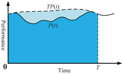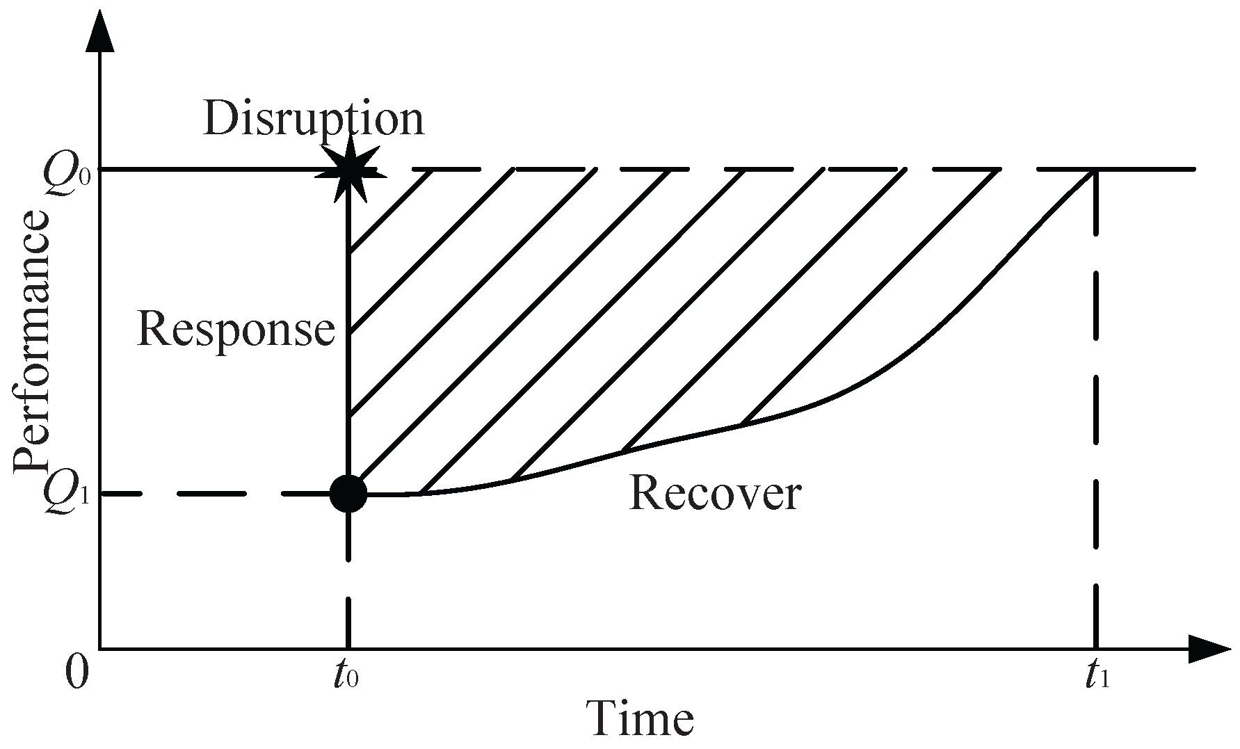Figure 1 shows the conceptual schematic diagram of the system’s resilience behavior. The figure shows a disruption occurring at time $t_0$, and the system performance degrades from $Q_0$ to $Q_1$. By taking appropriate action, the system finally returns to baseline at time $t_1$.

In a systematic review, Hohenstein et al. [7] summarized that “most research has been qualitative and lacks assessment and measurement of supply chain network resilience”. To measure resilience, the Multidisciplinary Center of Earthquake Engineering to Extreme Events (MCEER) [11] proposed a measure of addressing “resilience loss”. They defined a normalized system performance curve $Q\left(t\right)$, and used the integral of performance loss function from disruption followed by a gradual recovery to describe system resilience loss (i.e., the shadowed area in Figure 1). This measure considers both the robustness of the system against the disruption and the rapidity of the recovery process. In particular, Mari et al. [12] applied the expected disruption cost to measure the supply chain resilience, and this metric is an instance of the “resilience loss“ in the supply chain. Based on such work, Cimellaro et al. [13] provided a further extension to define the resilience as the integral of the area beneath the curve $Q\left(t\right)$, which is regarded as a direct measure of resilience itself. Accordingly, the loss of resilience should be minimized, and the resilience itself should be maximized. However, because the recovery time of different systems differs, these two measures cannot be used to compare resilience. To solve this problem, Reed et al. 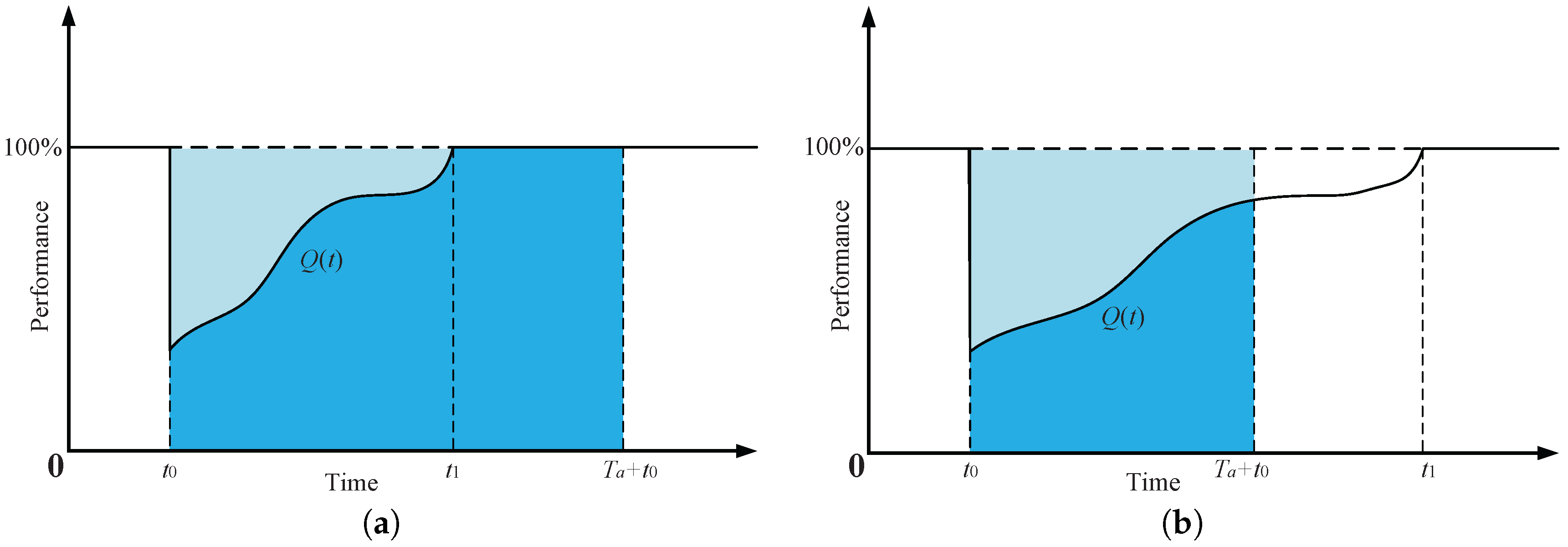[14] defined the resilience of a system as the ratio of the area beneath the curve $Q\left(t\right)$ to the time interval under consideration; Zobel [15] assumed that all systems will return to their original status before $T^{*}$ which serves as a strict upper bound on all possible recovery times, and defined “predicted resilience” as the ratio of the approximate area under the performance curve to $T^{*}$; Ouyang et al. [16] proposed a resilience measure as the ratio of the area under the real performance curve to that under the targeted performance curve over 0 to T; Spiegler et al. [17] applied the integral of time multiplied by the absolute error (ITAE) in the control engineering to measure the resilience of the supply chain network, where the error in the inventory (i.e., the difference between zero and the actual inventory) is calculated by analyzing the inventory levels and shipment rates. These measures allow system resilience to be compared on the same relative scale. However, (1) the $T^{*}$-based scale disregards the fact that not all systems have a strict upper bound on recovery time, and some systems cannot fully recover back; and (2) the lifetime-based one deviates from the original definition of resilience as “bounce back”.

In this paper, a new resilience measure is proposed. It involves using the maximum allowable recovery time as the time interval under consideration and providing a simulation-based estimation method. Our research benefits supply chain managers. When building a new supply chain network or changing the old one, supply chain managers can use our resilience measurement method to evaluate the resilience of the network design alternatives, verify whether the system resilience goal can be satisfied, and choose a resilient alternative that can withstand the disruption and return to the normal state quickly. The remainder of the paper is organized as follows. Section 2 describes the hierarchical structure of the supply chain network and its delivery mechanism. 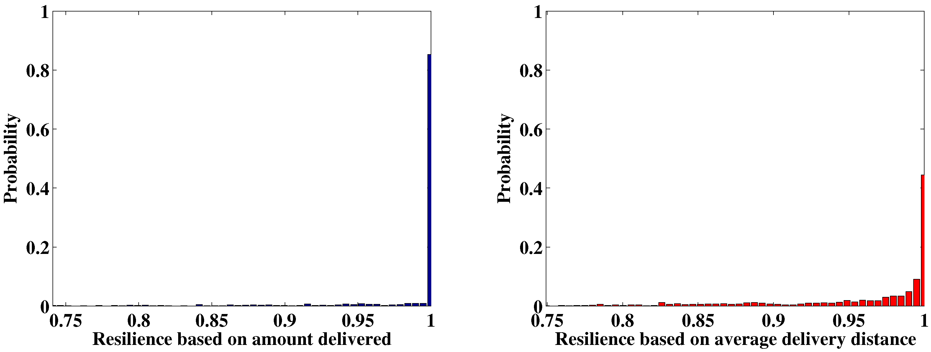In Section 3, the new resilience measure based on the maximum allowable recovery time is proposed, and two specific resilience measures for supply chain networks are provided. This is the resilience based on the amount of product delivered and the resilience based on the average delivery distance. 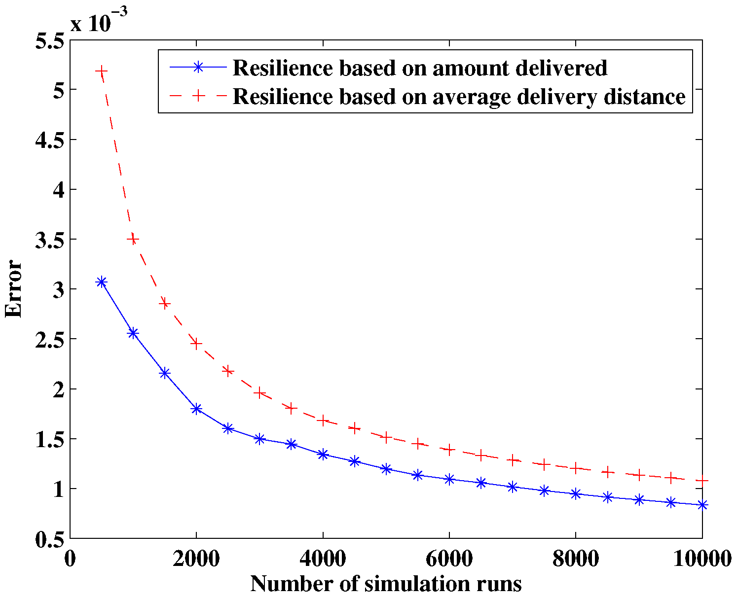Section 4 describes the development of a resilience simulation method based on the Monte Carlo method, and the simulation models, simulation flow and the error discussion are included. 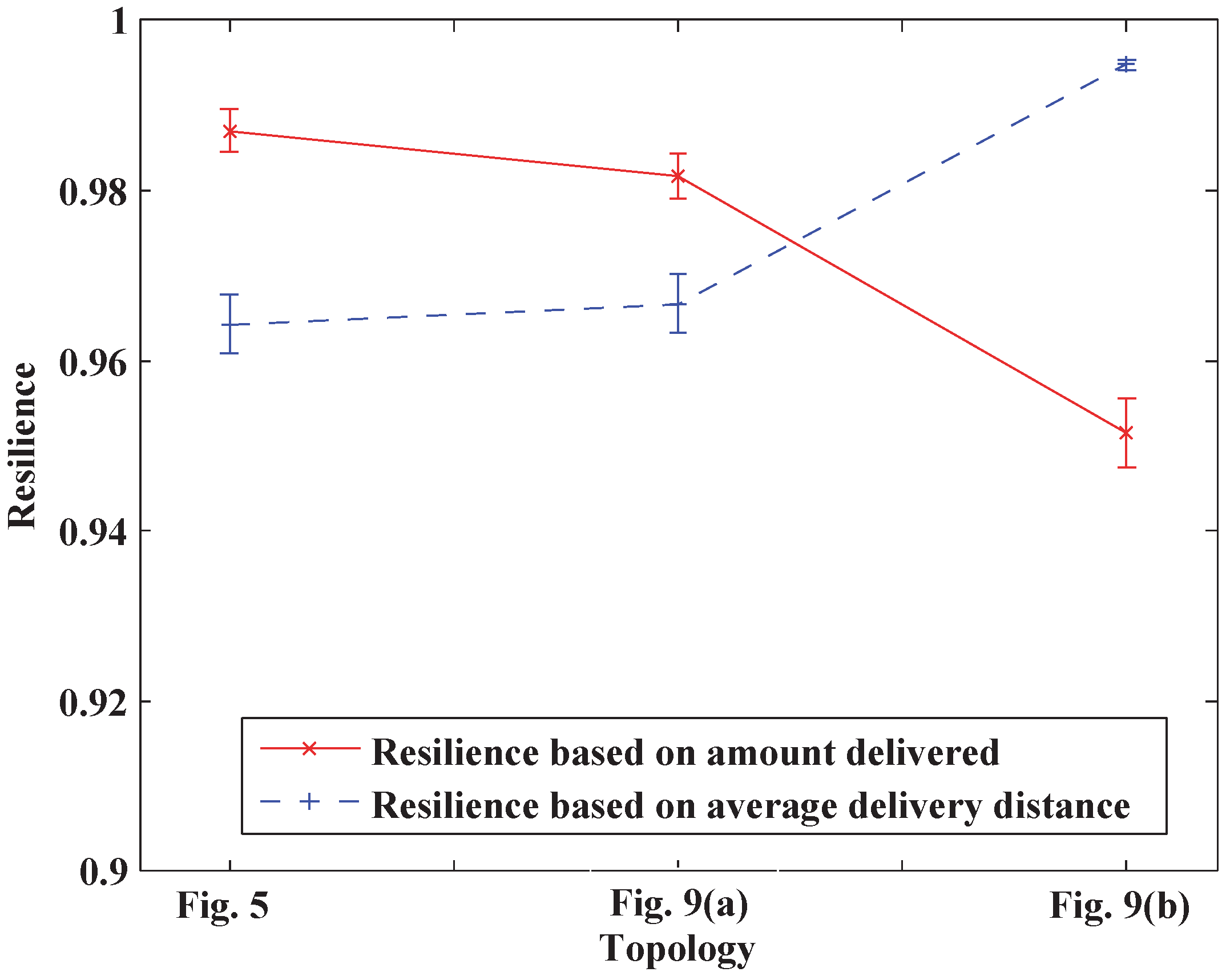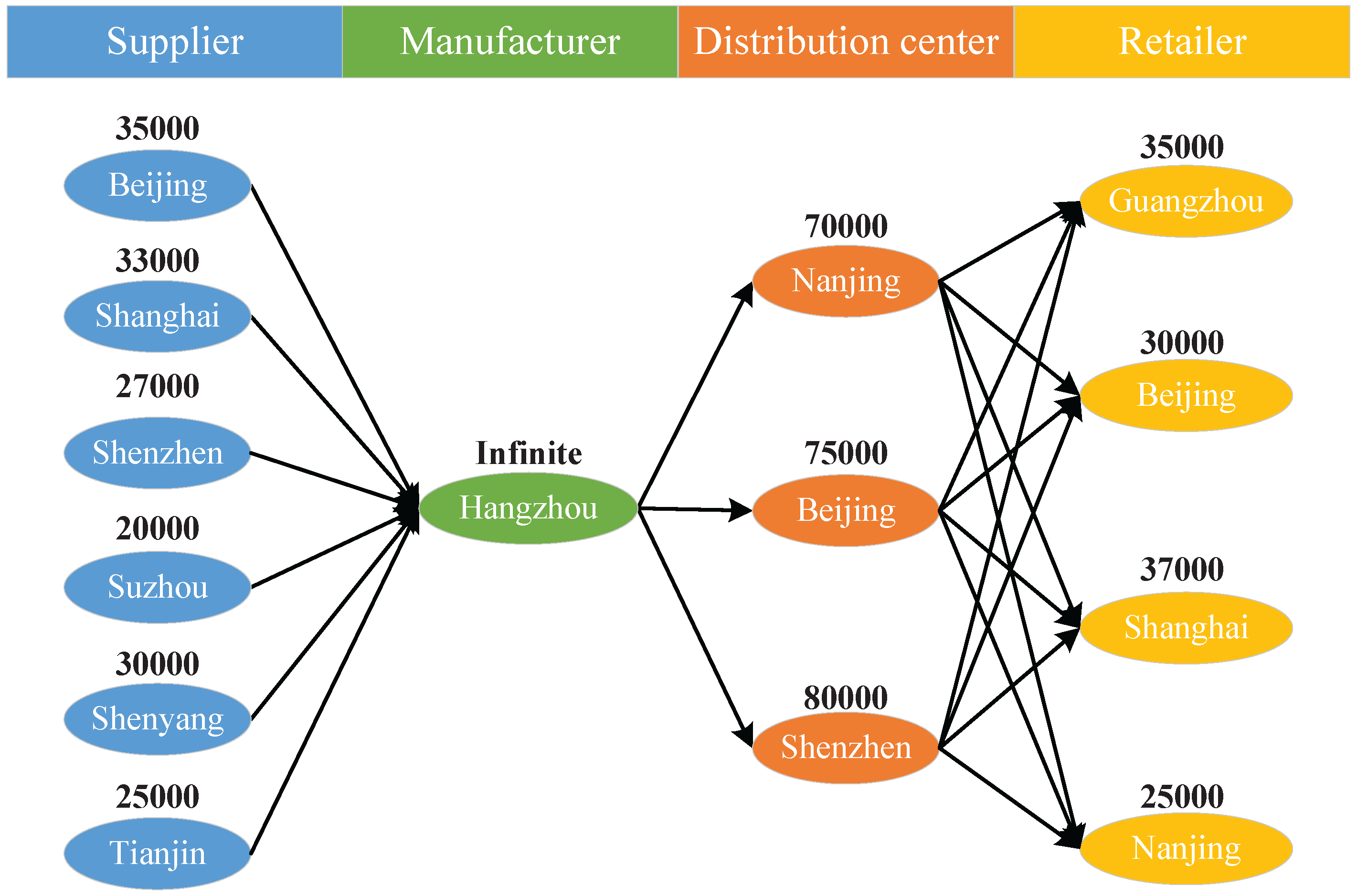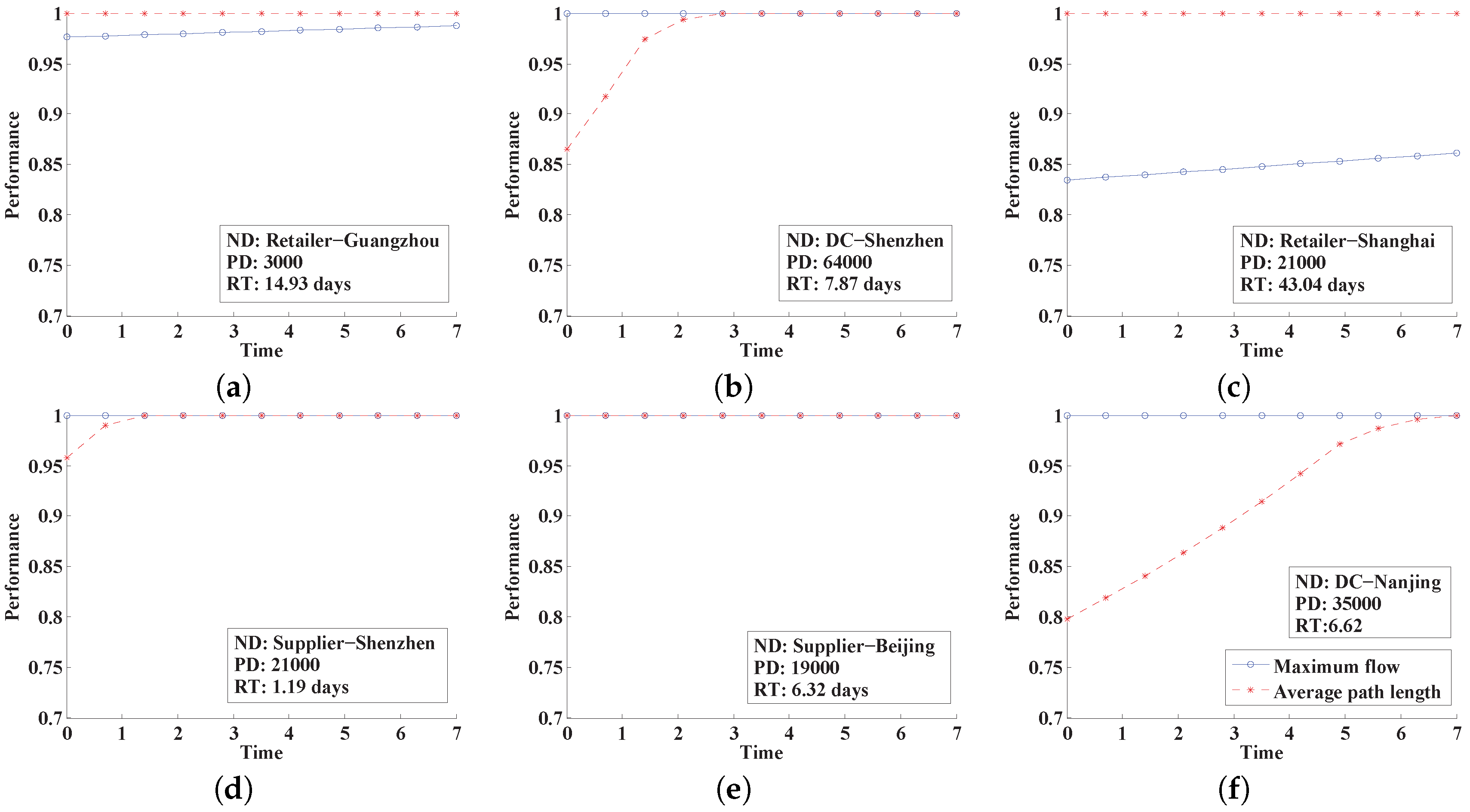In Section 5, a four-layered mobile phone supply chain network is introduced to show the effectiveness of our method, and the manner in which network topology affects the network resilience is discussed. Concluding remarks are provided in Section 6.

2. Problem

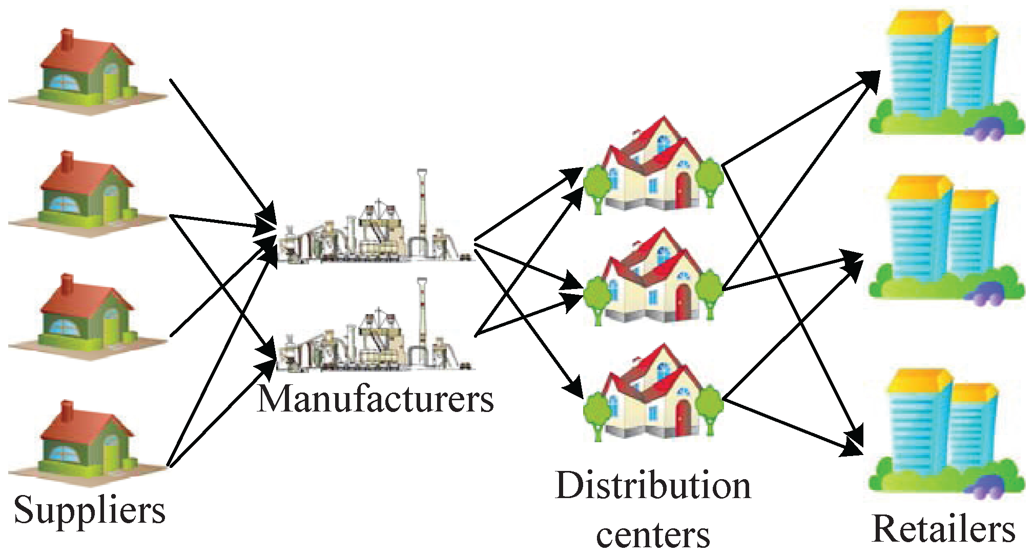
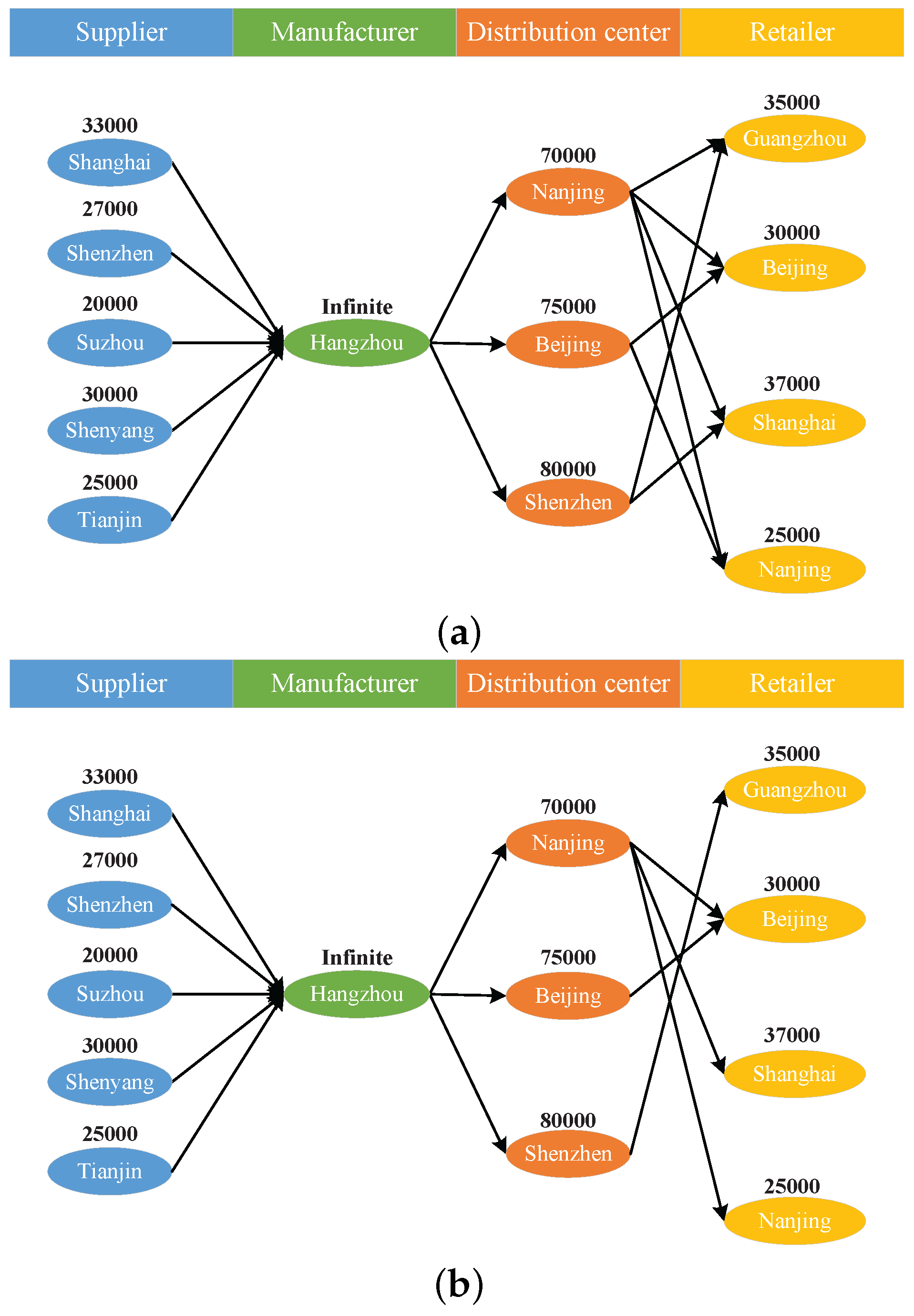
This paper considers hierarchical supply chain networks, as shown in Figure 2. In the network, all suppliers, manufacturers, distribution centers, retailers, and other involved institutions are considered as nodes, and nodes with the same function are grouped as one layer, e.g., supplier layer, manufacturer layer, distributor layer, retailer layer, etc. There may be a link between any pair of nodes in two adjacent layers for materials or product delivery, and the existence of links depends on the network topology planning. Note that, because nodes in different layers differ in functionality, links only exist between nodes in adjacent layers, i.e., the materials or products can only be transferred between adjacent layers (e.g., from a supplier to a manufacturer, from a manufacturer to a distribution center, and from a distribution center to a retailer) and not within the same layer.

The current paper focuses on measurement of the resilience of supply chain networks, and the following assumptions were made:

(1)

Only one type of product is produced and delivered per supply chain network.

(2)

Each node has a certain capacity, which can be used to produce and store productions. The link capacity is unlimited.

(3)

Both service time and waiting time on nodes are disregarded, and the waiting time on links is also disregarded.

(4)

Only nodes may suffer from the disruption, and there are no common-cause disruptions.

The first assumption is used to simplify the problem as Shin et al. [18], in which only one type of product is considered. For networks with multiple types of products, a similar method can be used by computing different resilience measures for different types of products, and then the system’s resilience can be synthetically calculated. Assumption 2 illustrates that the nodes are with finite manufacturing or restoration ability and the links have infinite delivery ability. Assumption 3 indicates that the materials and products are served immediately once they arrive at the node or link, and there is no waiting time. The service time on nodes in the same layer is always the same, so they are disregarded and only the delivery time on links is considered in our problem. The assumption that only nodes may suffer from the disruption is made here to simplify the discussion process, similar to the “perfect edges” assumption in the network reliability analysis [19,20,21], and can be easily extended by regarding links as nodes. The assumption that there would be “no common-cause disruption” means that one disruption can only cause the capacity of one node to degrade, which is similar to the widely used “no common-cause failure“ assumption in reliability research [22,23,24].

Hence, given the network topology, node capacities, node locations, disruptions, node capacity degradations and recovery time, the problem is to estimate the resilience of the supply chain network and verify whether the system resilience goal can be satisfied.

3. Resilience Measure of Supply Chain Networks

3.1. New Resilience Measure

Table 1. Comparisons of different resilience measures

No.	Reference	Measure	Formula	Conceptual Diagram	Problems	Our Measure Advantages
1	Bruneau et al. [11]	Resilience loss: the integral of the normalized performance loss function.	${\mathbb{R}}_L={\int }_{t_0}^{t_1}\left[1-Q\left(t\right)\right]dt$		Both measures cannot be used to compare the resilience of different systems as their relative scale, the recovery time ($t_1-t_0$), varies.	The maximum allowable recovery time determined by users is used as the time scale, which makes our measure comparable.
2	Cimellaro et al. [13]	Resilience: the integral of the normalized performance function.	${\mathbb{R}}_C={\int }_{t_0}^{t_1}Q\left(t\right)dt$
3	Reed et al. [14]	Resilience: the ratio of the area beneath the curve $Q\left(t\right)$ to the time interval under consideration.	${\mathbb{R}}_R=\frac{{\int }_{t_s}^{t_e}Q\left(t\right)dt}{t_e-t_s}$		The time interval under consideration ($t_e-t_s$) can be defined flexibly, and the measure is comparable when the time interval is fixed. However, the time interval determination method is not provided, and the physical meaning of the measure is not clear.	The time scale of our measure provides a clear physical meaning, i.e., the average normalized performance of the system within the allotted recovery time after the disruption.
4	Zobel [15]	Predicted resilience: the ratio of the area under the performance curve to the strict upper bound of the recovery time ($T^{*}$).	${\mathbb{R}}_Z=\frac{T^{*}-\frac{Q_{l}T}{2}}{T^{*}}$		The strict upper bound of the recovery time ($T^{*}$) is used as the end of the time interval under consideration, which makes the measure comparable. However, the measure ignores the situation in which the system cannot fully return to baseline.	The maximum allowable recovery time determined by users is used as the time scale of our measure, the system is not required to be fully recovered at the end of the time interval.
5	Ouyang et al. [16]	Resilience: the ratio of the area between the actual performance curve $P\left(t\right)$ and the time axis to the area between the target performance curve $TP\left(t\right)$ and the time axis from 0 to T.	${\mathbb{R}}_O=\frac{{\int }_0^{T}P\left(t\right)dt}{{\int }_0^{T}TP\left(t\right)dt}$		A long time interval from 0 to T is used as the time scale, which makes the measure comparable. However, the measure cannot reflect the ability of a system to bounce back after disruptions, and bounce back is the original meaning of the word “resilience”.	Our measure focuses on the system behavior after the disruption, and the time when the disruption occurs is used as the beginning of the time interval.

$Q\left(t\right)$ is the normalized system performance at time t ($0\%\le Q\left(t\right)\le 100\%$), $t_s$ and $t_e$ are endpoints of the time interval under consideration, $Q_l$ and T are the predicted performance loss and recovery time, $P\left(t\right)$ and $TP\left(t\right)$ are the actual performance curve and targeted performance curve of the system, respectively.

summarizes the most commonly used resilience measures. In Table 1, Measures 1 and 2 cannot be used to compare the resilience of different systems as the relative scale, the recovery time, varies; Measure 3 does not specify the time interval under consideration; Measure 4 ignores the fact that the recovery time does not always have a strict upper bound; and Measure 5 is a long-term measure, which does not directly reflect the ability of the system to bounce back after the disruption.

According to the analysis results above, (1) to make the resilience measure comparable, a fixed time interval needs to be defined with a proper physics meaning; (2) to reflect the ability of the system to bounce back after the disruption, the time when the disruption occurs should be used as the beginning of the time interval; and (3) to consider both scenarios that the system can or cannot restore within the given time interval, the system is not required to be fully recovered at the end of the time interval. Hence, the maximum allowable recovery time determined by users is used as the time interval under consideration, and the following new resilience measure is proposed:

$$\mathbb{R}=\frac{{\int }_{t_0}^{T_a+t_0}Q\left(t\right)dt}{T_a},$$

(1)

where $\mathbb{R}$ is the system resilience, $t_0$ is the time at which the disruption occurs and the performance of the system begins to decline, and $T_a$ is the maximum allowable recovery time determined by users. The advantages of our measure can be seen in the last column of Table 1. As shown in Figure 3, the system resilience in the presence of one specific disruption can be expressed as the ratio of the integral of $Q\left(t\right)$ within the maximum allowable recovery time $T_a$ (i.e., the dark area) to the integral of the performance in the normal state (i.e., the colored rectangle area). Figure 3 illustrates two typical situations, one in which the system performance returns to its initial level within the allotted recovery time, and the other in which it does not, where $t_1$ is the time that the system performance fully returns to the baseline.

Our resilience measure has four advantages:

(1)

Using the maximum allowable recovery time as the time interval under consideration, the resilience of different systems are comparable by using the same relative scales.

(2)

The proposed resilience measure describes the average normalized performance of the system within the maximum allowable recovery time after the disruption, which has a clear physical meaning.

(3)

The time interval under consideration starts at the time when the disruption occurs, lasts a specific period of time, depending on users’ recovery requirements, and it reflects the “bounce back“ ability of the system.

(4)

If the system performance cannot return to baseline within the maximum allowable system recovery time, its resilience is considered low, and the area of the performance loss is large.

As shown in Equation (1), the resilience measure is able to comprehensively represent the ability of the system to withstand the disruption and recover rapidly. Here, $0\le \mathbb{R}\le 1$, (1) when $\mathbb{R}=1$, it means that the system has perfect resilience: either its performance degradation is 0 or it can recover from disruption instantaneously; (2) when $\mathbb{R}=0$, it indicates that the system is completely destroyed immediately upon disruption (i.e., its performance degrades to 0 at $t_0$) and cannot recover within the maximum allowable recovery time; and (3) it is obvious that systems with higher $\mathbb{R}$ are more resilient.

Equation (1) is a deterministic resilience measure that can be used to estimate system resilience in response to a certain disruption without uncertainty. In reality, the disruption, performance degradation and recovery time are all random variables, so engineers care more about the probabilistic resilience, which captures the stochastic behavior of the system during the design process. Because the analytical distribution of the system resilience is difficult to derive, we develop the expected system resilience as follows:

$$E\left(\mathbb{R}\right)=\frac{E\left[{\int }_{t_0}^{T_a+t_0}Q\left(t\right)dt\right]}{T_a}.$$

(2)

With N disruption samples, the average here served as the estimate for the expected system resilience, which produces the following:

$$\widehat{E\left(\mathbb{R}\right)}\approx \frac{{\displaystyle \sum _{i=1}^N}{\mathbb{R}}_i}{N},$$

(3)

where ${\mathbb{R}}_i$ is the system resilience under the ith disruption. With the resilience data obtained from N disruptions, the distribution of the system resilience can also be built, and the probabilistic resilience of the system can be obtained.

The resilience measures can be used during both the design and operation stages of the supply chain network. In the design stage, because of the lack of real data, the simulation method is the most effective means of analyzing the supply chain’s resilience process after possible disruptions. The histogram of the network resilience can be obtained using the Monte Carlo based resilience simulation. Equation (7) can be used to estimate the expected network resilience and verify whether the resilience goal is satisfied. If not, the supply chain managers need to improve the network resilience by reducing the capacity degradation, speeding the recovery rate, choosing better recovery scheme, or changing the network topology, etc. In addition, the network topology and recovery strategy can be further optimized using the resilience estimation results. In the operation stage, the performance data of the supply chain network can be monitored. When a disruption occurs, the performance data can be collected, and the network resilience under the certain disruption can be estimated using Equation (6). Because the occurrence of disruptions is relatively infrequent, the deterministic resilience measure is usually used in the operational stage.

3.2. Resilience Measures for Supply Chain Networks

As shown in Equation (1), the resilience of the system depends on its performance degradation and recovery behavior, which changes along with the disruption. The most important step to determine the resilience measure for a specific system is to find its key performance indexes (KPIs). In particular, for supply chain networks, customers care whether the products can be delivered to them as required, so the amount of product delivered W and the average delivery distance $\overline{D}$ are set as KPIs. The amount of product delivered indicates the degree to which the supply chain network satisfies the customers’ demands, and the average delivery distance determines both cost and time of the product delivery.

The amount of product delivered is the maximum amount of product that can be delivered from the first layer to the last (e.g., from suppliers to retailers) within the supply chain network. It is the maximum flow in the Graph Theory, and many algorithms have been developed to solve the maximum flow problem. These include the Edmonds and Karp algorithm [25] and Preflow–Push algorithm [26].

The average delivery distance is defined as the ratio of the delivery distances of all products on the network to the number of products, i.e.,

$$\overline{D}=\frac{1}{W}{\displaystyle \sum _{i=1}^N}{\displaystyle \sum _{j=1}^n}{w}_{ij}{d}_{ij},$$

(4)

where n is the number of nodes on the network, $d_{ij}$ is the distance between nodes pair i and j, and $w_{ij}$ is the amount of product delivered on the link between nodes i and j.

According to Equation (1), the performance used in the system resilience calculation needs to be normalized. The initial system performance is considered as $Q_0=100\%$, so the normalized amount of product delivered and average delivery distance at time t can be calculated as follows:

$$Q_W\left(t\right)=\frac{W\left(t\right)}{W\left(t_0\right)}\mathrm{and}{Q}_D\left(t\right)=\frac{\overline{D}\left(t_0\right)}{\overline{D}\left(t\right)},$$

(5)

where $W\left(t\right)$ and $\overline{D}\left(t\right)$ are the amount of product delivered and the average delivery distance at time t, and $W\left(t_0\right)$ and $\overline{D}\left(t_0\right)$ are the initial performances at time $t_0$. Note that the amount of product delivered is a the-larger-the-better parameter and the average delivery distance is a the-smaller-the-better parameter, so their normalized performances are calculated differently.

Combining Equations (5) with (1) shows the two deterministic resilience expressions for supply chain networks as follows:

$${\mathbb{R}}_W=\frac{{\int }_{t_0}^{T_a+t_0}{Q}_W\left(t\right)dt}{T_a}\mathrm{and}{\mathbb{R}}_D=\frac{{\int }_{t_0}^{T_a+t_0}{Q}_D\left(t\right)dt}{T_a}.$$

(6)

The expected resilience of the supply chain network can be estimated as follows:

$$\widehat{E\left({\mathbb{R}}_W\right)}\approx \frac{{\displaystyle \sum _{i=1}^N}{\mathbb{R}}_{W_i}}{N}\mathrm{and}\widehat{E\left({\mathbb{R}}_D\right)}\approx \frac{{\displaystyle \sum _{i=1}^N}{\mathbb{R}}_{D_i}}{N},$$

(7)

where ${\mathbb{R}}_{W_i}$ and ${\mathbb{R}}_{D_i}$ are the resilience based on the amount of product delivered and the resilience based on the average delivery distance under the ith disruption, respectively.

4. Resilience Estimation Using Simulation

Because supply chains have networked structures, no analytical model has been proposed for the network flow analysis, which leaves Monte Carlo based simulation a valuable method. Deleris and Erhun [27] used the Monte Carlo method to assess the volume loss due to disruptions in supply networks. Colicchia et al. [28] used a simulation-based framework to assess the effectiveness of their proposed risk management methods. Klibi and Martel [29] also proposed a Monte Carlo approach to generate scenarios incorporating both random and extreme events for risk modeling on supply chain networks. Schmitt and Singh [8] used a simulation model to generalize the impact of disruptions on supply chain networks and focused on the downtime and recovery of the system. However, the resilience measures used in these works are different from those used here, and the KPI average delivery distance has not been studied thoroughly in any previous work. Hence, this section describes the development of a resilience estimation method based on Monte Carlo simulation for supply chain networks.

4.1. Simulation Models

4.1.1. Structure-Based Models

Adjacency matrixes were used here to describe the topology of the supply chain network and the capacity, flow, and distance of each link. To make calculation easier, two virtual nodes, i.e., a source node and a destination node, were added to produce a virtual network, where the source and the destination are connected to all the nodes at the input and output layers of the real network (e.g., all sites of suppliers and retailers in Figure 2), respectively. Hence, the total number of nodes in the network is increased to $m=n+2$ (including the two virtual nodes), where the source node is denoted as Node 1 and the destination node as Node m.

These structure-based models are as follows:

$$\begin{array}{c}{A}_m=\left(\begin{array}{cccc}{a}_{11}& a_{12}& \cdots & a_{1m}\\ a_{21}& a_{22}& \cdots & a_{2m}\\ ⋮& & & \\ a_{m1}& a_{m2}& \cdots & a_{mm}\end{array}\right)C_m=\left(\begin{array}{cccc}{c}_{11}& c_{12}& \cdots & c_{1m}\\ c_{21}& c_{22}& \cdots & c_{2m}\\ ⋮& & & \\ c_{m1}& c_{m2}& \cdots & c_{mm}\end{array}\right)\hfill \\ W_m=\left(\begin{array}{cccc}{w}_{11}& w_{12}& \cdots & w_{1m}\\ w_{21}& w_{22}& \cdots & w_{2m}\\ ⋮& & & \\ w_{m1}& w_{m2}& \cdots & w_{mm}\end{array}\right)D_m=\left(\begin{array}{cccc}{d}_{11}& d_{12}& \cdots & d_{1m}\\ d_{21}& d_{22}& \cdots & d_{2m}\\ ⋮& & & \\ d_{m1}& d_{m2}& \cdots & d_{mm}\end{array}\right),\hfill \end{array}$$

(8)

where $A_m$ is the topology matrix, and $a_{ij}=\left\{\begin{array}{c}0,\mathrm{no}\mathrm{link}\mathrm{between}\mathrm{nodes}i\mathrm{and}j\hfill \\ 1,\mathrm{a}\mathrm{link}\mathrm{exists}\mathrm{between}\mathrm{nodes}i\mathrm{and}j\hfill \end{array}\right.$, $C_m$, $W_m$ and $D_m$ are capacity matrix, flow matrix and distance matrices, $c_{ij}$, $w_{ij}$ and $d_{ij}$ are the capacity, flow (i.e., the amount of product delivered), and length of the link between nodes i and j, respectively. According to Assumption 2 in Section 2, the capacity of links is infinite, while each node has a finite capacity. It is obvious that the capacity of the nodes actually bounds that of the links, giving the following:

$$c_{ij}=min(c_i,c_j),$$

(9)

where $c_i$ and $c_j$ are the capacity of nodes i and j, respectively.

4.1.2. Flow Distribution Model

Usually, the supply chain networks have some redundancy, which means that there is more than one possible flow distribution that can support the amount of product to be delivered by the network (i.e., the maximum flow). To reduce the delivery time and cost, the products are always delivered with the minimal average delivery distance. To find such flow distribution, a linear programming model is constructed as follows:

$$min\overline{D}=\frac{1}{W}{\displaystyle \sum _{i=1}^m}{\displaystyle \sum _{j=1}^m}{w}_{ij}{d}_{ij},$$

(10)

subjected to

$${\displaystyle \sum _{i=1}^m}{w}_{1i}={\displaystyle \sum _{i=1}^m}{w}_{im}=W,$$

(11)

$${\displaystyle \sum _{i=1}^m}{w}_{ij}={\displaystyle \sum _{i=1}^m}{w}_{ji}(\mathrm{for}1<j<m),$$

(12)

$$0\le w_{ij}\le c_{ij}.$$

(13)

In the model, Equation (11) is the constraint of the maximum flow, Equation (12) is the constraint for the flow conservation, and Equation (13) is the capacity constraint.

4.1.3. Resilience Estimation Model

Because of the difficulties in the continuous performance data monitoring and the integral calculation in Equation (1), a numerical method is applied as follows:

$${\int }_{t_0}^{T_a+t_0}Q\left(t\right)dt\approx \frac{{\displaystyle \sum _{k=1}^s}\left[Q\left(t_k\right)+Q\left(t_{k-1}\right)\right]\Delta t}{2},$$

(14)

where $\Delta t$ is the time granularity, i.e., a width of the time interval, s is the number of $\Delta t$ in the allowable recovery range $T_a$ ($s=T_a/\Delta t$), and $Q\left(t_k\right)$ is the normalized system performance at the end of the kth $\Delta t$ ($t_k=k\Delta t$). The time granularity should be chosen properly. If it is too large, the result will not be accurate enough; if it is too small, the resilience computation will be time-consuming.

Combining Equation (14) with Equation (6), the resilience based on the amount of product delivered and on the average delivery distance of the supply chain network due to a certain disruption can be calculated as follows:

$${\mathbb{R}}_W\approx \frac{{\displaystyle \sum _{k=1}^s}\left[Q_W\left(t_k\right)+Q_W\left(t_{k-1}\right)\right]\Delta t}{2T_a}\mathrm{and}{\mathbb{R}}_D\approx \frac{{\displaystyle \sum _{k=1}^s}\left[Q_D\left(t_k\right)+Q_D\left(t_{k-1}\right)\right]\Delta t}{2T_a}.$$

(15)

4.1.4. Sampling Model

The Monte Carlo method is used here to produce samples for the three types of random variables in the current problem, including the disruption time, the performance degradation, and the recovery time. Given the cumulative distribution function (CDF) $F\left(x\right)$ for each random variable X, the samples can be generated using the inverse function method: $X=F^{-1}\left(U\right)$, where U is a uniform random number between 0 and 1 [30]. Inverse functions for some typical distributions can be seen in

Table 2. Inverse functions for some typical distributions.

Type	Function	Inverse
Uniform distribution	$F\left(x\right)=\frac{x-a}{b-a}$	$F^{-1}\left(x\right)=(b-a)U+a$
Exponential distribution	$F\left(x\right)=1-e^{\lambda x}$	$F^{-1}\left(x\right)=\frac{-ln\left(U\right)}{\lambda }$
Normal distribution	$F\left(x\right)=\mathrm{\Phi }\left(\frac{x-\mu }{\sigma }\right)$	$F^{-1}\left(x\right)=z_U\sigma +\mu$
Lognormal distribution	$F\left(x\right)=\mathrm{\Phi }\left(\frac{ln\left(x\right)-\mu }{\sigma }\right)$	$F^{-1}\left(x\right)=e^{z_U\sigma +\mu }$

$z_U$ is the value on the z-axis for which $U\times 100\%$ of the area under the z curve lies to the right of $z_U$, i.e., the $100\left(1-U\right)$th percentile of the standard normal distribution.

.

4.2. Simulation Flow

Using the Monte Carlo method, the resilience of the supply chain network can be estimated as shown in Figure 4, with the following steps:

(1)

Calculate the initial performance $W\left(t_0\right)$ and $\overline{D}\left(t_0\right)$ of the supply chain network, which is the performance of the supply chain network before the disruption occurs (i.e., under normal state).

(2)

Use the Monte Carlo method to randomly determine the disruption time for all nodes, and identify the node at which the first disruption occurs.

(3)

Determine the capacity degradation and recovery time of the node on which the first disruption occurs by random sampling of their corresponding distributions.

(4)

Calculate the network performance $W\left(t\right)$ and $\overline{D}\left(t\right)$ at every $\Delta t$ time interval.

(5)

Compute the resilience of supply chain network under the certain disruption using Equation (15).

(6)

Repeat Steps (2)–(5) N iterations.

(7)

Estimate the expected resilience of the supply chain network using Equation (7), and obtain the corresponding resilience histogram.

In the simulation, the disruption occurrence is event based, and the network resilience calculation is activity based.

4.3. Error

Samples $x_i$ obtained using Monte Carlo simulation from one population are identical and identically distributed (i.i.d.) random variables. According to the Central Limit Theorem, if the variance of the i.i.d. variables is finite, the arithmetic average of the samples follows a normal distribution with mean μ and variance $\frac{{\sigma }^2}{N}$ for large sample size N. The error of estimation can be calculated as follows:

$$\epsilon =\left|X-\widehat{X}\right|<\frac{z_{\alpha /2}\sigma }{\sqrt{N}},$$

(16)

where $\widehat{X}$ is the estimate of X, and $\widehat{X}=\frac{\sum x_i}{N}$, $1-\alpha$ is the confidence level (e.g., $1-\alpha =95\%$).

In the current problem, combining Equations (7) and (16) produces the following:

$${\epsilon }_{E\left({\mathbb{R}}_W\right)}=\left|E\left({\mathbb{R}}_W\right)-\widehat{E\left({\mathbb{R}}_W\right)}\right|<\frac{z_{\alpha /2}{S}_{{\mathbb{R}}_W}}{\sqrt{N}}\mathrm{and}{\epsilon }_{E\left({\mathbb{R}}_D\right)}=\left|E\left({\mathbb{R}}_D\right)-\widehat{E({\mathbb{R}}_D})\right|<\frac{z_{\alpha /2}{S}_{{\mathbb{R}}_D}}{\sqrt{N}},$$

(17)

where $S_{{\mathbb{R}}_W}$ and $S_{{\mathbb{R}}_D}$ are the standard deviations of ${\mathbb{R}}_W$ and ${\mathbb{R}}_D$, respectively. The standard deviations of the samples are used as the unbiased estimates of variance.

5. Case Study

5.1. Case Overview

This case concerns a mobile phone supply chain network with four levels of nodes adapted from [31]. As Figure 5 shows, there are six suppliers, located in Beijing, Shanghai, Shenzhen, Suzhou, Shenyang and Tianjin; one manufacturer, in Hangzhou; three distribution centers, in Beijing, Nanjing and Shenzhen; and four retailers, in Beijing, Shanghai, Guangzhou, and Nanjing. In this case, all the suppliers, manufacturers, distribution centers and retailers are considered as nodes, and their abilities (i.e., the supply ability of suppliers, the manufacturing capacity of the manufacturer, the transformative ability of distribution centers, and the demand from retailers) are considered the capacity of the nodes. Figure 5 shows all possible links and the capacity of all nodes. The distances between node pairs are obtained from the flight information as shown in

Table 3. Distances between suppliers and the manufacturer (km).

	Suppliers	Beijing	Shanghai	Shenzhen	Suzhou	Shenyang	Tianjin
Manufacturer
Hangzhou		1663	179	1100	121	1310	1036

,

Table 4. Distances between the manufacturer and distribution centers (km).

	Distribution Centers	Nanjing	Beijing	Shenzhen
Manufacturer
Hangzhou		254	1663	1070

and

Table 5. Distances between distribution centers and retailers (km).

	Retailers	Guangzhou	Beijing	Shanghai	Nanjing
Distribution Centers
Nanjing		1125	900	255	0
Beijing		1900	0	1062	900
Shenzhen		105	1930	1210	1160

.

When a disruption occurs at one node, the capacity of that node decreases, which may decrease the amount of product delivered or the average delivery distance of the network. As the node capacity returns to baseline, the network performance does as well. In the current problem, the node capacity recovery rate is constant. The goals of the expected resilience based on the amount of product delivered and the one based on the average delivery distance are both 0.96 under the maximum allowable recovery time as seven days, i.e., $T_a=7$ days. The node disruption time follows the exponential distribution, which is usually used in the previous study of the supply chain, see [32,33]. The node capacity degradation follows the discrete distribution, which is usually used in the stochastic flow network analysis (see [34,35]). The node recovery time follows either lognormal distribution or uniform distribution. The lognormal distribution is used as the repair time of systems always follows such distribution (see [36,37,38]). The uniform distribution is used to reflect the adaptability of our method to different distributions. The parameters of these distributions are shown in

Table 6. Distribution parameters of the case.

Type	Location	Disruption Time (Days)	Recovery Time (Days)	Capacity Degradation
Suppliers	Beijing	X∼$E\left(0.009\right)$	$ln\left(X\right)$∼$N(3.5,{1.5}^2)$
	Shanghai	X∼$E\left(0.010\right)$	$ln\left(X\right)$∼$N(3.3,{1.5}^2)$
	Shenzhen	X∼$E\left(0.015\right)$	$ln\left(X\right)$∼$N(2.7,{1.5}^2)$
	Suzhou	X∼$E\left(0.022\right)$	$ln\left(X\right)$∼$N(2,{1.5}^2)$
	Shenyang	X∼$E\left(0.018\right)$	$ln\left(X\right)$∼$N(3,{1.5}^2)$
	Tianjin	X∼$E\left(0.015\right)$	$ln\left(X\right)$∼$N(2.5,{1.5}^2)$	$P_i\left(1000x\right)=\frac{1000}{c_i},$
Manufacturer	Hangzhou	X∼$E\left(0.020\right)$	$ln\left(X\right)$∼$N(3,{1.5}^2)$
Distribution centers	Nanjing	X∼$E\left(0.1\right)$	X∼$U[4,10]$	$(x=1,2,...,\frac{c_i}{1000})$
	Beijing	X∼$E\left(0.03\right)$	X∼$U[4,10]$
	Shenzhen	X∼$E\left(0.05\right)$	X∼$U[4,10]$
Retailers	Guangzhou	X∼$E\left(0.015\right)$	$ln\left(X\right)$∼$N(3.5,{1.5}^2)$
	Beijing	X∼$E\left(0.009\right)$	$ln\left(X\right)$∼$N(3,{1.5}^2)$
	Shanghai	X∼$E\left(0.010\right)$	$ln\left(X\right)$∼$N(3.7,{1.5}^2)$
	Nanjing	X∼$E\left(0.015\right)$	$ln\left(X\right)$∼$N(2.5,{1.5}^2)$

. It is obvious that the resilience evaluation results will be influenced by the types of probability distributions. However, our resilience measurement method is still valid, as it is very convenient to change the distribution types in the Monte Carlo based simulation.

5.2. Resilience Evaluation

Using the simulation method detailed in Section 4, the resilience of the mobile phone supply chain network can be estimated, and some typical resilience behaviors of the network after a disruption are illustrated in Figure 6 ($\Delta t=0.7$ days).

As shown in Figure 6, one can see that the disruption on one node may cause the performance degradation and recovery of the network along with the node. Using the optimization model in Section 4.1.2, the flow distribution that supports the maximum flow with the minimal average delivery distance can be found, and the extra capacity of each node is defined as the “node redundant capacity”, which can be calculated by subtracting the flow distributed to it in the initial state from its total capacity. It is here noted that, due to the node capacity redundancy, the network may recover fully before the node. As shown in Figure 6b, the distribution center Shenzhen needs $7.87$ days to recover from this disruption, and the network recovers completely after $2.34$ days. In this case, the flow distribution returns to the initial state when the capacity of the distribution center Shenzhen returns to $\mathrm{35,000}$, which is the flow distributed to such a node in the initial state (i.e., the node has a 45,000 capacity redundancy). Nodes with less redundancy are more important. For example, when the disruption occurs for any retailer, which has no capacity redundancy either in itself or in the layer, the amount of product delivered within the network will drop (see Figure 6a,c); when this happens to suppliers in Shanghai, Shenzhen, Suzhou, and Tianjin or the distribution center in Nanjing, which show some capacity redundancy in the layer but none in itself, the average delivery distance will decline, as these nodes provide the minimal delivery distance (Figure 6d,f); when it occurs on the supplier in Beijing, which itself is a redundancy and does not participate in the initial flow distribution, both the amount of product delivered and the average delivery distance of the network retain their baseline values (see Figure 6e).

In the current case study, the number of iterations is 1000. After the simulation, the estimate of the expected system resilience was found to be $\widehat{E\left({\mathbb{R}}_W\right)}=0.987032$ and $\widehat{E\left({\mathbb{R}}_D\right)}=0.964301$, according to Equation (7). The histograms of both resilience are illustrated in Figure 7. Results indicate that both resilience distributions have long tails, the probability that the resilience based on the amount of product delivered was greater than 0.985 exceeds $80\%$, and resilience based on the average delivery distance was over $40\%$. Figure 7 shows the network resilience to be very high under most disruption conditions, and it also has some probability to be small in response to some disruptions. The histogram of the resilience based on the average delivery distance is flatter than resilience based on the amount of product delivered, which results in a lower estimate for the expected value of the resilience based on the average delivery distance in the network.

As described in Section 4.3, the resilience simulation errors decrease along with the simulation runs (Figure 8), and one can see that the simulation error is very small. Using our resilience measurement method, one can see that both of the two types of network resilience are satisfied (i.e., $\widehat{E\left({\mathbb{R}}_W\right)}>\widehat{E\left(R_W^{*}\right)}=0.96$ and $\widehat{E\left({\mathbb{R}}_D\right)}>\widehat{E\left(R_D^{*}\right)}=0.96$).

It is obvious that the network resilience differs for different topologies. In the current case study, two topologies were used for comparison, and their topological structures are illustrated in Figure 9. To facilitate the comparison, all the links that provide the minimal delivery distances in the fully connected topology of Figure 5 are reserved, and other redundancy links are reduced to some certain extent. Hence, all three of the topologies share the same initial performance, i.e., $W\left(t_0\right)=\mathrm{127,000}$ and $\overline{D}\left(t_0\right)=1613.2$ km. The capacity redundancy of the supply chain network is considered as the ratio of the total spare capacity over the total working capacity. Figure 5 shows the maximum redundancy, Figure 9b shows the minimal redundancy, and Figure 9a shows a middling system.

Using our proposed resilience measurement method, the network resilience of the three topologies is obtained and compared in Figure 10. For the three topologies, one can see that:

(1)

$\widehat{E\left({\mathbb{R}}_{W_5}\right)}>\widehat{E\left({\mathbb{R}}_{W_{9a}}\right)}>\widehat{E\left({\mathbb{R}}_{W_{9b}}\right)}$. In this case, the redundancy of the three topologies is “Figure 5 $>$ Figure 9a $>$ Figure 9b”, and $\widehat{E\left({\mathbb{R}}_{\mathbb{W}}\right)}$ declines along with the network redundancy. This phenomenon occurs because the network flow on the node under disruption has larger possibility to be migrated to other nodes in the network that have higher redundancy. It is also noted that the topology “Figure 9b“ cannot satisfy the goal of the expected resilience based on the amount of product delivered. In such a case, the supply chain network manager needs to improve the system resilience. In general, the supply chain network with more redundancy tends to have higher resilience based on the amount of product delivered, but it also depends on at which node the redundant capacity is located. To improve the network resilience based on the amount of product delivered, the redundant capacity needs to be allocated to proper nodes.

(2)

$\widehat{E\left({\mathbb{R}}_{D_5}\right)}<\widehat{E\left({\mathbb{R}}_{D_{9a}}\right)}<\widehat{E\left({\mathbb{R}}_{D_{9b}}\right)}$. In this case, $\widehat{E\left({\mathbb{R}}_{\mathbb{D}}\right)}$ increases along as the network redundancy decreases. However, in general, it is hard to tell how the resilience based on average delivery distance changes along with the network redundancy. As the average delivery distance of the network is determined by both the current amount of product delivered and the flow distribution (see Equation (4)), if the maximum flow of the network decreases during the disruption, i.e., the amount of product delivered decreases, it is hard to determine whether the resilience based on the average delivery distance will decrease or not.

The results of the simulation are consistent with expectations, which proves that the method is efficient.

6. Conclusions

This paper proposes a new resilience measure, in which the maximum allowable recovery time serves as the time interval under consideration, and two specific resilience measures, i.e., the resilience based on the amount of product delivered and the resilience based on average delivery distance, are provided for supply chain networks. A simulation method based on the Monte Carlo is developed to estimate the network resilience. The effectiveness of this method is verified using a mobile phone supply chain network. The contributions of the current paper include the following: (1) a new resilience measure is provided using the maximum allowable recovery time determined by customers as the time scale. It not only allows system resilience to be compared on the same relative scale but also provides a clear physical meaning focusing on the ability of “bounce back“ after disruptions; (2) two resilience measures are proposed for supply chain networks, one based on the amount of product delivered and the other on the average delivery distance, providing quantitative methods for supply chain networks whose resilience is usually qualitatively analyzed (Hohenstein et al. [7]); and (3) a resilience estimation framework is developed for supply chain networks, in which the Monte Carlo method based simulation and the graph theory are combined. A linear programming model is constructed under the constraint of flow conversations to determine the flow distribution with the minimal delivery distance.

In this paper, the current case study indicates that the topology of the network has a large influence on the system resilience, and the optimization of the network topology using the system resilience as constraints is slated for further study. Moreover, all the institutions (i.e., suppliers, manufacturers, distribution centers and retailers) are supposed to be controlled by the company’s supply chain manager. If not, each institution’s behavior will influence the resilience of the supply chain network. This problem will also be studied together with the Games Theory in our future work.

References

1. Rice, J.B.; Caniato, F. Building a secure and resilient supply network. Supp. Chain Manag. Rev. 2003, 7, 22–30. [Google Scholar]
2. Christopher, M.; Peck, H. Building the resilient supply chain. Int. J. Logist. Manag. 2004, 15, 1–13. [Google Scholar] [CrossRef] [Green Version]
3. Chopra, S.; Sodhi, M.S. Reducing the risks of supply chain disruptions. MIT Sloan Manag. Rev. 2014, 55, 73–80. [Google Scholar]
4. Henry, D.; Ramirez-Marquez, J.E. Generic metrics and quantitative approaches for system resilience as a function of time. Reliab. Eng. Syst. Saf. 2012, 99, 114–122. [Google Scholar] [CrossRef]
5. Sheffi, Y.; Rice, J.B. A Supply Chain View of the Resilient Enterprise. MIT Sloan Manag. Rev. 2005, 47, 41–48. [Google Scholar]
6. Ponomarov, S.Y.; Holcomb, M.C. Understanding the concept of supply chain resilience. Int. J. Logist. Manag. 2009, 20, 124–143. [Google Scholar] [CrossRef]
7. Hohenstein, N.O.; Feisel, E.; Hartmann, E.; Giunipero, L. Research on the phenomenon of supply chain resilience: A systematic review and paths for further investigation. Int. J. Phys. Distrib. Logist. Manag. 2015, 45, 90–117. [Google Scholar] [CrossRef]
8. Schmitt, A.J.; Singh, M. A quantitative analysis of disruption risk in a multi-echelon supply chain. Int. J. Prod. Econ. 2012, 139, 22–32. [Google Scholar] [CrossRef]
9. Xiao, R.; Yu, T.; Gong, X. Modeling and simulation of ant colony’s labor division with constraints for task allocation of resilient supply chains. Int. J. Artif. Intell. Tools 2012, 21, 1–19. [Google Scholar] [CrossRef]
10. Wu, T.; Huang, S.; Blackhurst, J.; Zhang, X.; Wang, S. Supply chain risk management: An agent-based simulation to study the impact of retail stockouts. IEEE Trans. Eng. Manag. 2013, 60, 676–686. [Google Scholar] [CrossRef]
11. Bruneau, M.; Chang, S.E.; Eguchi, R.T.; Lee, G.C.; O’Rourke, T.D.; Reinhorn, A.M.; Shinozuka, M.; Tierney, K.; Wallace, W.A.; von Winterfeldti, D. A Framework to Quantitatively Assess and Enhance the Seismic Resilience of Communities. Earthq. Spectra 2003, 19, 733–752. [Google Scholar] [CrossRef]
12. Mari, S.I.; Lee, Y.H.; Memon, M.S. Sustainable and Resilient Supply Chain Network Design under Disruption Risks. Sustainability 2014, 6, 6666–6686. [Google Scholar] [CrossRef]
13. Cimellaro, G.P.; Reinhorn, A.M.; Bruneau, M. Seismic resilience of a hospital system. Struct. Infrastruct. Eng. 2010, 6, 127–144. [Google Scholar] [CrossRef]
14. Reed, D.A.; Kapur, K.C.; Christie, R.D. Methodology for Assessing the Resilience of Networked Infrastructure. IEEE Syst. J. 2009, 3, 174–180. [Google Scholar] [CrossRef]
15. Zobel, C.W. Representing perceived tradeoffs in defining disaster resilience. Decis. Support Syst. 2011, 50, 394–403. [Google Scholar] [CrossRef]
16. Ouyang, M.; Dueñas-Osorio, L.; Min, X. A three-stage resilience analysis framework for urban infrastructure systems. Struct. Saf. 2012, 36–37, 23–31. [Google Scholar] [CrossRef]
17. Spiegler, V.L.M.; Naim, M.M.; Wikner, J. A control engineering approach to the assessment of supply chain resilience. Int. J. Prod. Res. 2012, 50, 6162–6187. [Google Scholar] [CrossRef]
18. Shin, K.; Shin, Y.; Kwon, J.H.; Kang, S.H. Risk propagation based dynamic transportation route finding mechanism. Ind. Manag. Data Syst. 2012, 112, 102–124. [Google Scholar] [CrossRef]
19. AboElFotoh, H.M.; Colbourn, C.J. Efficient algorithms for computing the reliability of permutation and interval graphs. Networks 1990, 20, 883–898. [Google Scholar] [CrossRef]
20. Patvardhan, C.; Prasad, V.C.; Pyara, V.P. Generation of K-Trees of Undirected Graphs. IEEE Trans. Reliab. 1997, 46, 208–211. [Google Scholar] [CrossRef]
21. Lin, M.S.; Ting, C.C. A polynomial-time algorithm for computing K-terminal residual reliability of d-trapezoid graphs. Inf. Process. Lett. 2015, 115, 371–376. [Google Scholar] [CrossRef]
22. Satyanarayana, A.; Chang, M.K. Network reliability and the factoring theorem. Networks 1983, 13, 107–120. [Google Scholar] [CrossRef]
23. Coit, D.W.; Smith, A.E. Reliability optimization of series-parallel systems using a genetic algorithm. IEEE Trans. Reliab. 1996, 45, 254–266. [Google Scholar] [CrossRef]
24. Hardy, G.; Lucet, C.; Limnios, N. K-terminal network reliability measures with binary decision diagrams. IEEE Trans. Reliab. 2007, 56, 506–515. [Google Scholar] [CrossRef]
25. Edmonds, J.; Karp, R.M. Theoretical improvements in algorithmic efficiency for network flow problems. J. ACM 1972, 19, 248–264. [Google Scholar] [CrossRef]
26. Goldberg, A.V.; Tarjan, R.E. A new approach to the maximum-flow problem. J. ACM 1988, 35, 921–940. [Google Scholar] [CrossRef]
27. Deleris, L.A.; Erhun, F. Risk management in supply networks using monte-carlo simulation. In Proceedings of the Winter Simulation Conference, Orlando, FL, USA, 4–7 December 2005.
28. Colicchia, C.; Dallari, F.; Melacini, M. Increasing supply chain resilience in a global sourcing context. Prod. Plan. Control 2010, 21, 680–694. [Google Scholar] [CrossRef]
29. Klibi, W.; Martel, A. Scenario-based supply chain network risk modeling. Eur. J. Operat. Res. 2012, 223, 644–658. [Google Scholar] [CrossRef]
30. Zio, E. Computational Methods for Reliability and Risk Analysis; Chapter Monte Carlo Simulation for Reliability and Availability Analysis; World Scientific: Singapore, 2009; pp. 59–69. [Google Scholar]
31. Liu, Y. Integrated Optimization of Design and Operation for Resilient Supply Chain Network under Disruption Risk. Master’s Thesis, Northeastern University, Boston, MA, USA, 2011. [Google Scholar]
32. Weiss, H.J.; Rosenthal, E.C. Optimal ordering policies when anticipating a disruption in supply or demand. Eur. J. Oper. Res. 1992, 59, 370–382. [Google Scholar] [CrossRef]
33. Tomlin, B. On the value of mitigation and contingency strategies for managing supply chain disruption risks. Manag. Sci. 2006, 52, 639–657. [Google Scholar] [CrossRef]
34. Lin, Y.K. System reliability of a stochastic-flow network through two minimal paths under time threshold. Int. J. Prod. Econ. 2010, 124, 382–387. [Google Scholar] [CrossRef]
35. Lin, Y.K. Stochastic flow networks via multiple paths under time threshold and budget constraint. Comput. Math. Appl. 2011, 62, 2629–2638. [Google Scholar] [CrossRef]
36. Mi, J. Interval estimation of availability of a series system. IEEE Trans. Reliab. 1991, 40, 541–546. [Google Scholar] [CrossRef]
37. Upadhya, K.S.; Srinivasan, N. Availability of weapon systems with multiple failures and logistic delays. Int. J. Qual. Reliab. Manag. 2003, 20, 836–846. [Google Scholar] [CrossRef]
38. Myrefelt, S. The reliability and availability of heating, ventilation and air conditioning systems. Energy Build. 2004, 36, 1035–1048. [Google Scholar] [CrossRef]
Figure 1. The schematic representation of resilience.
Sustainability 09 00144 g001
Figure 2. Hierarchical supply chain networks.
Sustainability 09 00144 g002
Figure 3. The proposed resilience measure in two typical situations. (a) T a + t 0 t 1 ; and (b) T a + t 0 < t 1 .
Sustainability 09 00144 g003
Figure 4. Input and output of the resilience simulation for supply chain networks.
Sustainability 09 00144 g004
Figure 5. Case network, adapted from [31].
Sustainability 09 00144 g005
Figure 6. Network performance curves after the disruption occurs at (a) the retailer in Guangzhou; (b) the distribution center in Shenzhen; (c) the retailer in Shanghai; (d) the supplier in Shenzhen; (e) the supplier in Beijing; (f) the distribution center in Nanjing. Note: N D is the node at which the disruption occurs, P D is the capacity degradation of the node, R T is the recovery time of the node, and D C is the distribution center.
Sustainability 09 00144 g006
Figure 7. Histograms of the network resilience.
Sustainability 09 00144 g007
Figure 8. Estimation error changes along with the number of simulation runs.
Sustainability 09 00144 g008
Figure 9. Two more topologies used to compare resilience. (a) topology A; (b) topology B.
Sustainability 09 00144 g009
Figure 10. Network performance curves after the disruption ( N = 1000 .)
Sustainability 09 00144 g010