Hesitant Trapezoidal Fuzzy QUALIFLEX Method and Its Application in the Evaluation of Green Supply Chain Initiatives

Abstract

This paper explores how to handle multiple criteria decision-making (MCDM) problems in which the criteria values of alternatives take the form of comparative linguistic expressions. Firstly, the new concept of hesitant trapezoidal fuzzy numbers (HTrFNs) is provided to model the semantics of the comparative linguistic expressions. Then, the operational laws and the distance measures of HTrFNs are presented. Afterwards, a useful outranking method, the hesitant trapezoidal fuzzy QUALIFLEX method, is developed to handle the MCDM problems with hierarchical structure in the environment of HTrFN. At length, the proposed method is applied to evaluating green supply chain initiatives in order to achieve sustainable economic and environmental performance, and a case study concerned with a fashion retail chain is presented to demonstrate its feasibility and applicability, also, a comparative analysis with other relevant approaches is conducted to validate the effectiveness of the proposed method.

1. Introduction

With the increase of public awareness of the need to protect the environment, it is urgent for businesses to introduce and promote business practices that help ease the negative impacts of their actions on the environment [1]. Green supply chain management (GSCM) has proven to be a useful way for companies to obtain profit and market share objectives by lowering environmental impacts and improving ecological efficiency. In general, the GSCM initiatives consist of green manufacturing initiatives (such as green design), green supplier initiatives (such as environmentally-friendly raw materials), green logistics initiatives (such as green packaging), green marketing initiatives, etc. The successful implementation of suitable green initiatives could assist companies to generate higher revenues and improve their competitive advantages. However, how to choose appropriate GSCM initiatives is a complex task, which not only requires a trade-off between the benefits and cost involved, but also takes the operational and environmental performance into account [1]. This is a typical multiple criteria decision-making (MCDM) problem.

It is quite common that in the real-life world, decision-makers (DMs) employ linguistic terms to express their opinions for evaluating qualitative MCDM problems. For example, when evaluating the innovation capacity of a company that implements GSCM initiatives, the DMs may utilize the linguistic terms like “high” or “low” instead of numerical values to express their assessments. Zadeh [2] introduced the linguistic fuzzy approach to model such linguistic terms in the MCDM problems. Afterwards, the linguistic fuzzy approach has further been extended into several different linguistic models: the linguistic 2-tuple model [3,4], the symbolic linguistic model [5,6,7], the linguistic model based on the Type-2 fuzzy set [8], the proportional two 2-tuple model [9], the comparative linguistic expressions (CLEs) model based on the hesitant fuzzy linguistic term set (HFLTS) [10,11], etc.

The CLEs based on HFLTSs have been applied to different qualitative decision-making problems [10,11,12,13]. To address this kind of qualitative MCDM problem, Rodriguez et al. [10,11] introduced the linguistic intervals envelope of HFLTS to facilitate the computing with words process [14,15]. Liu and Rodriguez [13] proposed the trapezoidal fuzzy number (TrFN) envelope for HFLTS. However, these aforementioned envelopes of HFLTSs either lose their original fuzzy representation or are hard to derive. To conveniently deal with the CLEs based on HFLTSs in decision-making, in this paper, we will propose a new concept of hesitant trapezoidal fuzzy numbers (HTrFNs) to represent the semantic of the CLEs based on HFLTSs. The HTrFNs benefited from the superiority of both TrFNs and hesitant fuzzy elements (HFEs) are suitable to tackle the imprecise and ambiguous information in complex decision-making problems. To address the MCDM problems with HTrFNs data, it is important and urgent to develop effective decision-making approaches accordingly.

The QUALIFLEX (qualitative flexible multiple criteria method) originally developed by Paelinck [16] is one of the effective outranking methods to solve the MCDM problems. The QUALIFLEX method has recently been extended into various fuzzy decision environments, such as the decision environment of interval Type-2 TrFNs [17,18], the context of hesitant fuzzy sets [19], the context of intuitionistic fuzzy sets [20], the environment of interval-valued intuitionistic fuzzy sets [21,22], etc. Nevertheless, these previous QUALIFLEX methods fail to deal with the hierarchical MCDM problems with CLEs based on HTrFNs. Thus, in this paper, we will leverage the QUALIFLEX approach to develop a hesitant trapezoidal fuzzy QUALIFLEX method. We first present the concept of the signed distance of HTrFNs, and we further define a signed distance-based ranking method for comparing the magnitude of HTrFNs. The concordance/discordance indices are identified by the signed distance-based ranking method. Considering that the hesitant trapezoidal fuzzy MCDM problem is of a hierarchical structure, we further calculate the weighted concordance/discordance indices and the comprehensive concordance/discordance indices. Meanwhile, we select the classical TOPSIS method and the ELECTRE (ELimination Et Choix Traduisant la REalité) method as the benchmark methods to make a comparative analysis with the proposed method. To provide the additional contributions of the practical implications, this paper finally applies the proposed method to solve a green supply chain initiative evaluation problem.

The main contributions of this paper comprise the following five aspects: (1) the new concept of HTrFN and its basic operational laws are developed; (2) two kinds of hesitant trapezoidal fuzzy distance measures are proposed; (3) a new signed distance-based ranking method for HTrFNs is developed; (4) the hesitant trapezoidal fuzzy QUALIFLEX method is provided; (5) a case study concerned with the evaluation of green supply chain initiatives is conducted. The rest of the paper is organized as follows: Section 2 reviews the concepts of TrFNs, HFEs and HFLTSs and also introduces the new concept of HTrFNs. Section 3 develops a hesitant trapezoidal fuzzy QUALIFLEX approach to solve the hierarchical MCDM problems with HTrFNs. In Section 4, a case study is presented, and a comparative analysis with other relevant approaches is conducted. Section 5 presents our conclusions.

2. Preliminaries

This section reviews the concepts of TrFNs, HFEs and HFLTSs and introduces the new concept of HTrFN.

2.1. Some Useful Concepts

Definition 1.

A fuzzy number $\tilde{\alpha }=T(a,b,c,d)$ is said to be a TrFN [2] if its membership function is given as follows:

$${\mu }_{\tilde{\alpha }}(x)=\{\begin{array}{cc}(x-a)/(b-a),\hfill & \hfill (a\le x<b)\hfill \\ \hspace{0.17em}\hspace{0.17em}\hspace{0.17em}1,\hfill & \hfill (b\le x\le c)\hfill \\ (d-x)/(d-c),\hfill & \hfill (c<x\le d)\hfill \\ \hspace{0.17em}\hspace{0.17em}\hspace{0.17em}0,\hfill & \hfill otherwise\hfill \end{array}$$

(1)

where the closed interval $[b,c]$, $a$ and $d$ are the mode, lower and upper limits of $\tilde{\alpha }$, respectively.

Remark 1.

A TrFN $\tilde{\alpha }=T(a,b,c,d)$ is positive if $a>0$ or $a=0$ and $d>0$. A positive TrFN $\tilde{\alpha }=T(a,b,c,d)$ is the normalized TrFN if $d\le 1$, and thus, the TrFN $\tilde{1}=T(1,\hspace{0.17em}1,\hspace{0.17em}1,\hspace{0.17em}1)$ is the maximal normalized TrFN, which is also called the ideal TrFN. A TrFN $\tilde{\alpha }=T(a,b,c,d)$ is a real number if $a=b=c=d$. A TrFN $\tilde{\alpha }=T(a,b,c,d)$ is a triangular fuzzy number if $b=c$.

Usually, the TrFNs are good enough to capture the uncertainty and vagueness of linguistic terms, and the relationships between the linguistic term set with a seven-point rating scale and the TrFNs are shown in Table 1.

Table 1. Linguistic terms and the corresponding trapezoidal fuzzy numbers (TrFNs).

Ratings	Abbreviation	TrFNs
s0: Very poor	VP	T (0.0, 0.0, 0.1, 0.2)
s1: Poor	P	T (0.1, 0.2, 0.2, 0.3)
s2: Medium poor	MP	T (0.2, 0.3, 0.4, 0.5)
s3: Fair	F	T (0.4, 0.5, 0.5, 0.6)
s4: Medium good	MG	T (0.5, 0.6, 0.7, 0.8)
s5: Good	G	T (0.7, 0.8, 0.8, 0.9)
s6: Very good	VG	T (0.8, 0.9,1.0, 1.0)

In some real-life MCDM cases, the DMs may hesitate among several possible values to express their assessments. The hesitant fuzzy set (HFS) is a good tool to capture these hesitant situations, which is introduced as follows:

Definition 2.

Let $X$ be a reference set [23]; a HFS $Q$ on $X$ is defined in terms of a function $h_Q(x)$ when applied to $X$ returning a subset of $[0,1]$.

Xia and Xu [24] expressed the HFS by a mathematical symbol:

$$Q=\left\{<x,h_Q(x)>|x\in X\right\}$$

(2)

where $h_Q(x)$ is a set of some different values in $[0,1]$, representing the possible membership degrees of the element $x\in X$ to $Q$. For convenience, they called $h_Q(x)$ a hesitant fuzzy element (HFE), denoted by $h=\{{\gamma }^f|f=1,2,\cdots ,\#h\}$ ($\#h$ is the number of all elements in $h$).

Given three HFEs represented by $h$, $h_1$ and $h_2$, respectively, and letting $\lambda >0$, then the operations of HFEs are defined as [24]:

$$h_1\oplus h_2={\cup }_{{\gamma }_1\in h_1,{\gamma }_2\in h_2}\left\{{\gamma }_1+{\gamma }_2-{\gamma }_1{\gamma }_2\right\};h_1\otimes h_2={\cup }_{{\gamma }_1\in h_1,{\gamma }_2\in h_2}\left\{{\gamma }_1{\gamma }_2\right\};$$

$$\lambda h={\cup }_{\gamma \in h}\left\{1-{(1-\gamma )}^{\lambda }\right\};h^{\lambda }={\cup }_{\gamma \in h}\left\{{\gamma }^{\lambda }\right\}.$$

To handle the qualitative hesitant situations, Rodriguez et al. [10] introduced the concept of HFLTS, which is shown as below:

Definition 3.

Let $S$ be a linguistic term set, $S=\{s_0,\cdots ,s_g\}$ [10]; an HFLTS $H_S$ is an ordered finite subset of consecutive linguistic terms of $S$. Generally, the $H_S$ is denoted by $H_s=\{s_i,s_{i+1},\cdots ,s_j\}$ where $s_k\in S$ $(k=i,i+1,\cdots ,j)$.

Remark 2.

The HFLTS $H_S$ is reduced to the linguistic variable [2] if the HFLTS $H_S$ only contains a single linguistic term. Namely, the linguistic variable is the special case of the $H_S$ and the linguistic variable $s_i\in S$ can also be rewritten as an HFLTS $H_S=\{s_i\}$.

2.2. New Concept of Hesitant Trapezoidal Fuzzy Sets

Based on the concepts and operational laws of TrFNs and HFEs, we present a new concept of the hesitant trapezoidal fuzzy set, which is good enough to represent the vagueness of the HFLTS.

Definition 4.

Let $X$ be a fixed set; a hesitant trapezoidal fuzzy set $\tilde{Q}$ on $X$ is defined as:

$$\tilde{Q}=\left\{<x,{\tilde{h}}_{\tilde{Q}}(x)>|x\in X\right\}$$

(3)

where ${\tilde{h}}_{\tilde{Q}}(x)$ is a set of different normalized TrFNs, representing the possible membership degrees of the element $x\in X$ to $\tilde{Q}$.

For convenience, ${\tilde{h}}_{\tilde{Q}}(x)$ is called an HTrFN denoted by $\tilde{h}=\{{\tilde{\alpha }}^f|f=1,2,\cdots ,\#\tilde{h}\}$ where the ${\tilde{\alpha }}^f=T{(}_a{\gamma }^f,{\hspace{0.17em}}_b{\gamma }^f,{\hspace{0.17em}}_c{\gamma }^f,{\hspace{0.17em}}_d{\gamma }^f)$ is a normalized TrFN and $\#\tilde{h}$ is the number of all TrFNs in $\tilde{h}$.

Remark 3.

The HTrFN $\tilde{h}$ is a full HTrFN if ${\tilde{\alpha }}^f=\tilde{1}$ $(f=1,2,\cdots ,\#\tilde{h})$, which is denoted by $\tilde{\tilde{1}}=\{{\tilde{1}}_f=T(1,\hspace{0.17em}1,\hspace{0.17em}1,\hspace{0.17em}1)|f=1,2,\cdots ,\#\tilde{h}\}$. Obviously, the full HTrFN $\tilde{\tilde{1}}$ is the maximal HTrFN, which is also called the ideal HTrFN. The HTrFN $\tilde{h}$ is a TrFN if $\#\tilde{h}=1$. In other words, the TrFN is the special case of the HTrFN. The HTrFN $\tilde{h}$ is a hesitant triangular fuzzy number [25] if ${}_b{\gamma }^f{=}_c{\gamma }^f$ $(f=1,2,\cdots ,\#\tilde{h})$. According to the definition of HTrFNs, it is easy to note that HTrFNs are suitable to capture and represent the uncertainty and vagueness of the HFLTS.

Example 1.

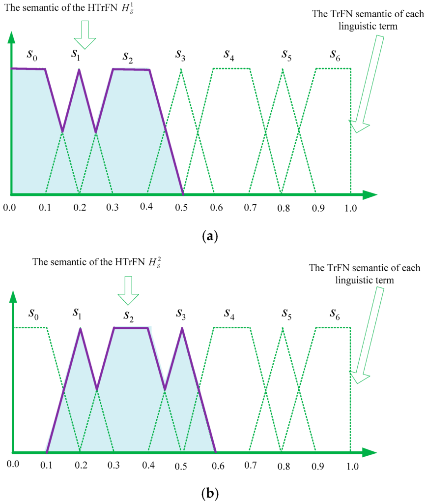
Let $S=\{s_0,s_1,s_2,s_3,s_4,s_5,s_6\}$ be a linguistic term set; the linguistic terms and the corresponding TrFNs are shown in Table 1. Given two HFLTSs $H_S^1=\{s_0,s_1,s_2\}$ and $H_S^2=\{s_1,s_2,s_3\}$, their semantics can be captured by the following two HTrFNs:

$${\tilde{h}}_1=\left\{\begin{array}{l}T(0,0,0.1,0.2),T(0.1,0.2,0.2,0.3),\\ T(0.2,0.3,0.4,0.5)\end{array}\right\}\iff H_S^1;$$

$${\tilde{h}}_2=\left\{\begin{array}{l}T(0.1,0.2,0.2,0.3),T(0.2,0.3,0.4,0.5),\\ T(0.4,0.5,0.5,0.6)\end{array}\right\}\iff H_S^2;$$

and the relations between the two HFLTSs and their corresponding HTrFNs are depicted in Figure 1.

Figure 1. The hesitant fuzzy linguistic term sets (HFLTSs) and the corresponding hesitant trapezoidal fuzzy numbers (HTrFNs): (a) under the case $H_S^1=\{s_0,s_1,s_2\}$; (b) under the case $H_S^2=\{s_1,s_2,s_3\}$ .

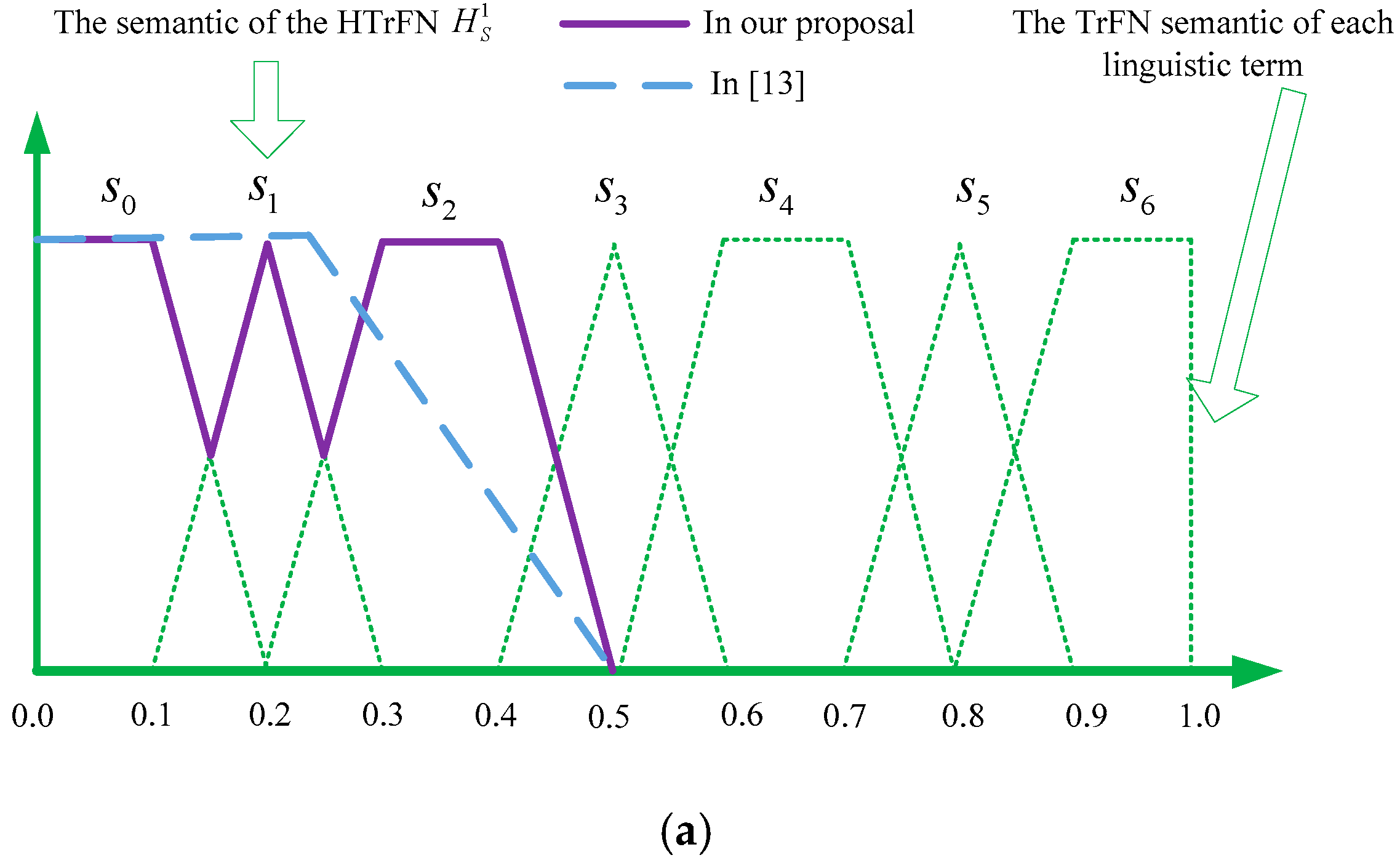
As far as we know, Liu and Rodríguez [13] suggested the use of TrFNs to capture the vagueness of HFLTSs, and the TrFNs envelopes of $H_S^1$ and $H_S^2$ are obtained as below:

$${env}_F(H_S^1)=T(0,0,0.239,0.5),{env}_F(H_S^2)=T(0.1,0.28,0.42,0.6).$$

We put the results obtained by the proposed method and Liu and Rodriguez’s [13] proposal in Figure 2 in order to provide a better view of the comparison results.

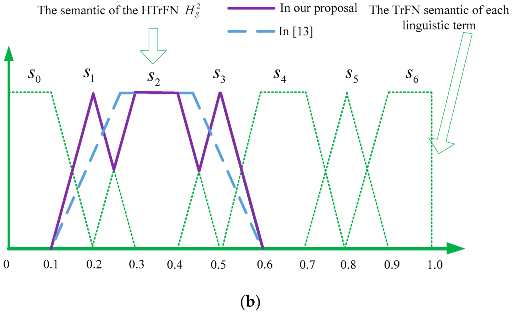
Figure 2. The results obtained by two different methods: (a) under the case $H_S^1=\{s_0,s_1,s_2\}$; (b) under the case $H_S^2=\{s_1,s_2,s_3\}$ .

It can be easily seen from Figure 2 that the HTrFNs take the semantics of each linguistic term of the HFLTSs into account; while Liu and Rodriguez’s [13] proposal uses the TrFNs to represent the semantics of HFLTS, which is relatively complex because the TrFNs are obtained by aggregating the fuzzy membership functions of the linguistic terms of the HFLTS using the OWA (ordered weighted averaging) aggregation operator.

Inspired by the operations on HFEs and TrFNs, we present the basic operations of HTrFNs.

Definition 5.

Let $\tilde{h}$, ${\tilde{h}}_1$ and ${\tilde{h}}_2$ be three HTrFNs; some operations of HTrFNs are defined as:

(1)

$\lambda \tilde{h}={\cup }_{\tilde{\alpha }\in \tilde{h}}\left\{T\left(1-{(1{-}_a\gamma )}^{\lambda },1-{(1{-}_b\gamma )}^{\lambda },1-{(1{-}_c\gamma )}^{\lambda },1-{(1{-}_d\gamma )}^{\lambda }\right)\right\}$ $(\lambda >0)$;

(2)

${\tilde{h}}^{\lambda }={\cup }_{\tilde{\alpha }\in \tilde{h}}\left\{T\left({{(}_a\gamma )}^{\lambda },{{(}_b\gamma )}^{\lambda },{{(}_c\gamma )}^{\lambda },{{(}_d\gamma )}^{\lambda }\right)\right\}$ $(\lambda >0)$;

(3)

${\tilde{h}}_1\oplus {\tilde{h}}_2={\cup }_{{\tilde{\alpha }}_1\in {\tilde{h}}_1,{\tilde{\alpha }}_2\in {\tilde{h}}_2}\left\{T\left(\begin{array}{l}{}_a{\gamma }_1{+}_a{\gamma }_2{-}_a{\gamma }_1{\times }_a{\gamma }_2,{\hspace{0.17em}}_b{\gamma }_1{+}_b{\gamma }_2{-}_b{\gamma }_1{\times }_b{\gamma }_2,\hspace{0.17em}\\ {}_c{\gamma }_1{+}_c{\gamma }_2{-}_c{\gamma }_1{\times }_c{\gamma }_2,{\hspace{0.17em}}_d{\gamma }_1{+}_d{\gamma }_2{-}_d{\gamma }_1{\times }_d{\gamma }_2\end{array}\right)\right\}$;

(4)

${\tilde{h}}_1\otimes {\tilde{h}}_2={\cup }_{{\tilde{\alpha }}_1\in {\tilde{h}}_1,{\tilde{\alpha }}_2\in {\tilde{h}}_2}\left\{T\left({}_a{\gamma }_1{\times }_a{\gamma }_2,{\hspace{0.17em}}_b{\gamma }_1{\times }_b{\gamma }_2,{\hspace{0.17em}}_c{\gamma }_1{\times }_c{\gamma }_2,{\hspace{0.17em}}_d{\gamma }_1{\times }_d{\gamma }_2\right)\right\}$.

Proposition 1.

Let $\tilde{h}$, ${\tilde{h}}_1$ and ${\tilde{h}}_2$ be three HTrFNs, then:

(1)

${\tilde{h}}_1\oplus {\tilde{h}}_2={\tilde{h}}_2\oplus {\tilde{h}}_1$;

(2)

${\tilde{h}}_1\otimes {\tilde{h}}_2={\tilde{h}}_2\otimes {\tilde{h}}_1$;

(3)

$\lambda ({\tilde{h}}_1\oplus {\tilde{h}}_2)=\lambda {\tilde{h}}_1\oplus \lambda {\tilde{h}}_2$ $(\lambda >0)$;

(4)

${({\tilde{h}}_1\otimes {\tilde{h}}_2)}^{\lambda }={\tilde{h}}_1^{\lambda }\otimes {\tilde{h}}_2^{\lambda }$ $(\lambda >0)$;

(5)

$({\lambda }_1+{\lambda }_2)\tilde{h}={\lambda }_1\tilde{h}\oplus {\lambda }_2\tilde{h}$ $({\lambda }_1,{\lambda }_2>0)$;

(6)

${\tilde{h}}^{({\lambda }_1+{\lambda }_2)}={\tilde{h}}^{{\lambda }_1}\otimes {\tilde{h}}^{{\lambda }_2}$ $({\lambda }_1,{\lambda }_2>0)$.

According to Definition 4, it is not hard to obtain the conclusions in Proposition 1 (the proof is omitted).

It is worthwhile to point out that the number of TrFNs in different HTrFNs may be different. In such cases, we should extend the shorter one until both of them have the same length when we compare them. To extend the shorter one, the best way is to add some TrFNs in it. Inspired by the similar techniques in [26,27,28], we extend the shorter one by adding the TrFN in it which mainly depends on the DMs’ risk preferences. The optimists anticipate the desirable outcomes and may add the maximum TrFN, while the pessimists expect the unfavorable outcomes and may add the minimum TrFN. Here, we employ the sign distance method [29] to compare the magnitude of TrFNs and further to identify the maximum TrFN or minimum TrFN.

Next, two distance measures for HTrFNs are proposed as follows:

Definition 6.

Given two HTrFNs ${\tilde{h}}_i=\left\{{\tilde{\alpha }}_i^f=T\left({}_a{\gamma }_i^f,{\hspace{0.17em}}_b{\gamma }_i^f,{\hspace{0.17em}}_c{\gamma }_i^f,{\hspace{0.17em}}_d{\gamma }_i^f\right)|f=1,2,\cdots ,\#{\tilde{h}}_i\right\}(i=1,2)$ with $\#\tilde{h}$ $=\#{\tilde{h}}_1=\#{\tilde{h}}_2$, the hesitant trapezoidal Hamming distance between them is defined as:

$$d_H\left({\tilde{h}}_1,{\tilde{h}}_2\right)=\frac{1}{6\#\tilde{h}}\left({\displaystyle \sum _{f=1}^{\#\tilde{h}}\left(\begin{array}{l}\left|{}_a{\gamma }_1^f{-}_a{\gamma }_2^f\right|+2\left|{}_b{\gamma }_1^f{-}_b{\gamma }_2^f\right|\\ +2\left|{}_c{\gamma }_1^f{-}_c{\gamma }_2^f\right|+\left|{}_d{\gamma }_1^f{-}_d{\gamma }_2^f\right|\end{array}\right)}\right)$$

(4)

and the hesitant trapezoidal Euclidean distance between them is defined as:

$$d_E\left({\tilde{h}}_1,{\tilde{h}}_2\right)=\sqrt{\frac{1}{6\#\tilde{h}}\left({\displaystyle \sum _{f=1}^{\#\tilde{h}}\left(\begin{array}{l}{\left({}_a{\gamma }_1^f{-}_a{\gamma }_2^f\right)}^2+2{\left({}_b{\gamma }_1^f{-}_b{\gamma }_2^f\right)}^2\\ +2{\left({}_c{\gamma }_1^f{-}_c{\gamma }_2^f\right)}^2+{\left({}_d{\gamma }_1^f{-}_d{\gamma }_2^f\right)}^2\end{array}\right)}\right)}$$

(5)

It is easy to prove that they are metric, and here, the processes of the proof are omitted.

Furthermore, we define the signed distance of HTrFNs and present a signed distance-based ranking approach to compare the magnitude of HTrFNs:

Definition 7.

Let $\tilde{h}=\left\{{\tilde{\alpha }}^f=T{(}_a{\gamma }^f,{\hspace{0.17em}}_b{\gamma }^f,{\hspace{0.17em}}_c{\gamma }^f,{\hspace{0.17em}}_d{\gamma }^f)|f=1,2,\cdots ,\#\tilde{h}\right\}$ be an HTrFN and $\tilde{\tilde{1}}$ be the ideal HTrFN, then the signed distance between $\tilde{h}$ and $\tilde{\tilde{1}}$ is defined as:

$$d_S(\tilde{h},\tilde{\tilde{1}})=\frac{1}{6\#\tilde{h}}{\displaystyle \sum _{f=1}^{\#\tilde{h}}\left(6{-}_a{\gamma }^f-2_b{\gamma }^f-2_c{\gamma }^f{-}_d{\gamma }^f\right)}$$

(6)

For two HTrFNs ${\tilde{h}}_1$ and ${\tilde{h}}_2$, it is easy to note that their signed distances $d_S({\tilde{h}}_1,\tilde{\tilde{1}})$ and $d_S({\tilde{h}}_2,\tilde{\tilde{1}})$ are real numbers, and they satisfy linear ordering, namely one of the following three conditions must hold: $d_S({\tilde{h}}_1,\tilde{\tilde{1}})>d_S({\tilde{h}}_2,\tilde{\tilde{1}})$, $d_S({\tilde{h}}_1,\tilde{\tilde{1}})=d_S({\tilde{h}}_2,\tilde{\tilde{1}})$, or $d_S({\tilde{h}}_1,\tilde{\tilde{1}})<d_S({\tilde{h}}_2,\tilde{\tilde{1}})$.

Thus, a signed distance-based ranking approach for HTrFNs is introduced as below:

(1)

if $d_S({\tilde{h}}_1,\tilde{\tilde{1}})>d_S({\tilde{h}}_2,\tilde{\tilde{1}})$, then ${\tilde{h}}_1\prec {\tilde{h}}_2$;

(2)

if $d_S({\tilde{h}}_1,\tilde{\tilde{1}})<d_S({\tilde{h}}_2,\tilde{\tilde{1}})$, then ${\tilde{h}}_1\succ {\tilde{h}}_2$;

(3)

if $d_S({\tilde{h}}_1,\tilde{\tilde{1}})=d_S({\tilde{h}}_2,\tilde{\tilde{1}})$, then ${\tilde{h}}_1\sim {\tilde{h}}_2$.

3. Hesitant Trapezoidal Fuzzy QUALIFLEX Analysis Method

This section establishes a decision-making environment based on HTrFNs for a hierarchical MCDM problem in which the criteria values take the form of CLEs and further presents a hesitant trapezoidal fuzzy QUALIFLEX method to solve such a hierarchical MCDM problem.

3.1. Description of the Hierarchical MCDM Problem with HTrFNs

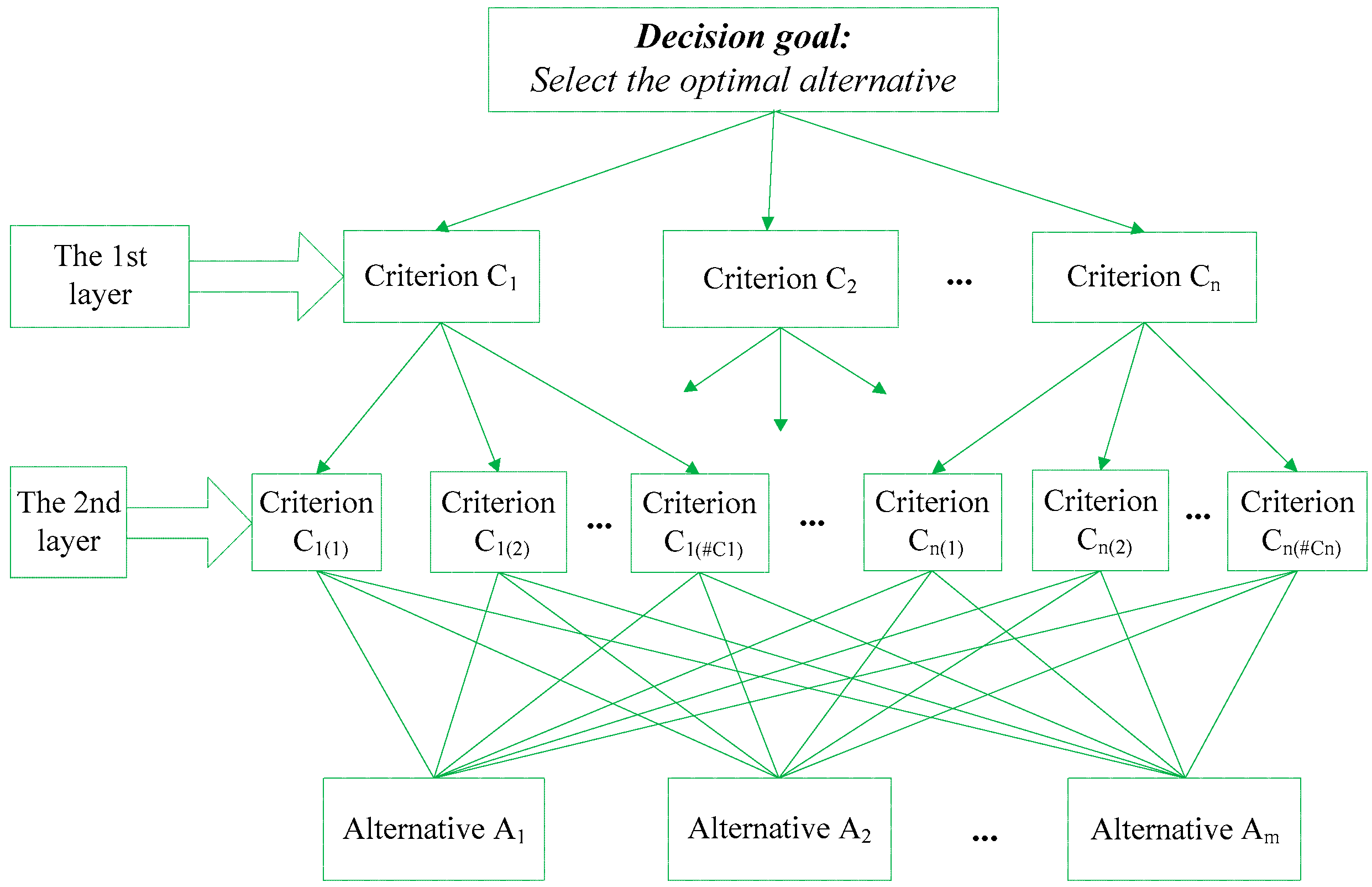
The MCDM is usual to find the best compromise solution from a set of feasible alternatives characterized with multiple competing criteria. This study focuses on a hierarchical MCDM problem with a two-layer structure, which usually involves a given set of main criteria and the corresponding sets of sub-criteria. The framework of the hierarchical MCDM problem is shown in Figure 3.

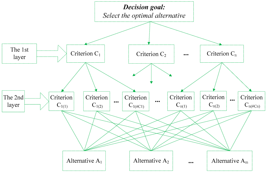
Figure 3. The framework of the hierarchical multiple criteria decision-making (MCDM) problem.

We assume that such a hierarchical MCDM problem includes $m$ alternatives $A_i$ $(i=1,2,\cdots ,m)$ and $n$ main criteria $C_j$$(j=1,2,\cdots ,n)$. Each main criterion $C_j$ has $\#C_j$ sub-criteria $C_{j(k)}(k=1,2,\cdots ,\#C_j)$, where $\#C_j$ denotes the number of sub-criteria in the main criterion $C_j$. The total number of sub-criteria is equal to ${\displaystyle {\sum }_{j=1}^n\#C_j}$. The DM evaluates the alternatives with respect to each sub-criterion of each main criterion using the CLEs, which can be captured by HTrFNs. From a computational point of view, the MCDM problem with CLEs is equivalent to the MCDM problem in the HTrFN context. Each criterion value takes the form of an HTrFN, and the alternative $A_i$ $(i=1,2,\cdots ,m)$ is evaluated with respect to the sub-criterion $C_{j(k)}(k=1,2,\cdots ,\#C_j)$ of the main criterion $C_j$ $(j=1,2,\cdots ,n)$. Let ${\tilde{h}}_{ij(k)}$ represent the criterion value of the $i\mathrm{th}$ alternative under the $k\mathrm{th}$ sub-criterion of the $j\mathrm{th}$ main criterion and be denoted by ${\tilde{h}}_{ij(k)}=\{T{(}_a{\gamma }_{ij(k)}^f,{\hspace{0.17em}}_b{\gamma }_{ij(k)}^f,{\hspace{0.17em}}_c{\gamma }_{ij(k)}^f,{\hspace{0.17em}}_d{\gamma }_{ij(k)}^f)$ $|f=1,2,\cdots ,\#{\tilde{h}}_{ij(k)}\}$. Let $w_j$ denote the weight of the main criterion $C_j$ and $w_{j(k)}$ represent the weight of the sub-criterion $C_{j(k)}$, and they satisfy the normalization conditions: $0\le w_j,w_{j(k)}\le 1$ $(j=1,2,\cdots ,n,k=1,2,\cdots ,\#C_j)$, ${\displaystyle {\sum }_{j=1}^n{w}_j}=1$ and ${\displaystyle {\sum }_{k=1}^{\#C_j}{w}_{j(k)}}=1$ $(j=1,2,\cdots ,n)$. Thus, the hierarchical MCDM problem with the two-layer structure in the HTrFN context can be concisely expressed in an HTrFN decision matrix as:

$$\mathit{H}={({\tilde{h}}_{ij(k)})}_{m\times n\times (\#c_n)}$$

(7)

3.2. The Proposed Method

In what follows, a hesitant trapezoidal fuzzy QUALIFLEX method is proposed to effectively solve the aforementioned hierarchical MCDM problem. This approach starts with the computation of the concordance/discordance index based on the successive permutations of all possible rankings of alternatives. Considering that the decision information takes the form of HTrFNs, this study utilizes a signed distance-based ranking approach introduced in Section 2 to compute the corresponding concordance/discordance index.

For the set of alternatives $\mathit{A}=$ $(A_1,$ $A_2,\cdots ,$ $A_m)$, there exist $m!$ permutations of the ranking of all alternatives. Let $P_{\rho }$ denote the $\rho \mathrm{th}$ permutation as:

$$P_{\rho }=(\dots ,A_{\xi },\dots ,A_{\zeta },\dots ), \rho =1,2,\cdots ,m!$$

(8)

where $A_{\xi },A_{\zeta }\in \mathit{A}$ and the alternative $A_{\xi }$ is ranked higher than or equal to $A_{\zeta }$.

Therefore, the concordance/discordance index ${\varphi }_{j(k)}^{\rho }(A_{\xi },A_{\zeta })$ for each pair of alternatives $(A_{\xi },A_{\zeta })$, at the level of preorder according to the $k\mathrm{th}$ sub-criterion within the $j\mathrm{th}$ main criterion and the ranking corresponding to the $\rho \mathrm{th}$ permutation, can be defined as:

$${\varphi }_{j(k)}^{\rho }(A_{\xi },A_{\zeta })=d_S({\tilde{h}}_{\zeta j(k)},\tilde{\tilde{1}})-d_S({\tilde{h}}_{\xi j(k)},\tilde{\tilde{1}})$$

(9)

where $d_S(•,\tilde{\tilde{1}})$ is the signed distance of HTrFNs defined in Equation (6).

From Equation (9), we can conclude that:

(1) If ${\varphi }_{j(k)}^{\rho }(A_{\xi },A_{\zeta })>0$, i.e., $d_S({\tilde{h}}_{\xi j(k)},\tilde{\tilde{1}})<d_S({\tilde{h}}_{\zeta j(k)},\tilde{\tilde{1}})$, then $A_{\xi }$ ranks over $A_{\zeta }$ under the $k\mathrm{th}$ sub-criterion within the $j\mathrm{th}$ main criterion; thus, there is concordance between the signed distance-based ranking orders and the preorders of $A_{\xi }$ and $A_{\zeta }$;

(2) If ${\varphi }_{j(k)}^{\rho }(A_{\xi },A_{\zeta })=0$, i.e., $d_S({\tilde{h}}_{\xi j(k)},\tilde{\tilde{1}})=d_S({\tilde{h}}_{\zeta j(k)},\tilde{\tilde{1}})$, then both $A_{\xi }$ and $A_{\zeta }$ have the same rank in the signed distance-based ranking;

(3) If ${\varphi }_{j(k)}^{\rho }(A_{\xi },A_{\zeta })<0$, i.e., $d_S({\tilde{h}}_{\xi j(k)},\tilde{\tilde{1}})>d_S({\tilde{h}}_{\zeta j(k)},\tilde{\tilde{1}})$, then $A_{\zeta }$ ranks over $A_{\xi }$; thus, there is discordance between the signed distance-based ranking orders and the preorders of $A_{\xi }$ and $A_{\zeta }$.

Thus, the three cases of the concordance/discordance index ${\varphi }_{j(k)}^{\rho }(A_{\xi },A_{\zeta })$ can be rewritten as:

$${\varphi }_{j(k)}^{\rho }(A_{\xi },A_{\zeta })=\{\begin{array}{l}{d}_S({\tilde{h}}_{\zeta j(k)},\tilde{\tilde{1}})-d_S({\tilde{h}}_{\xi j(k)},\tilde{\tilde{1}})>0\iff there is concordance\\ d_S({\tilde{h}}_{\zeta j(k)},\tilde{\tilde{1}})-d_S({\tilde{h}}_{\xi j(k)},\tilde{\tilde{1}})=0\iff there is ex aequo\\ d_S({\tilde{h}}_{\zeta j(k)},\tilde{\tilde{1}})-d_S({\tilde{h}}_{\xi j(k)},\tilde{\tilde{1}})<0\iff there is discordance\end{array}$$

(10)

Furthermore, considering that the aforementioned MCDM problem is of a two-layer structure, which usually can be reflected only when the aggregations of the weighted values within each main criterion and sub-criterion are conducted [1,30], therefore, taking into account the importance weight $w_{j(k)}$ of each sub-criterion $C_{j(k)}$ within the $j\mathrm{th}$ main criterion, the weighted concordance/discordance index ${\varphi }_j^{\rho }(A_{\xi },A_{\zeta })$ for each pair of alternatives $(A_{\xi },A_{\zeta })$, at the level of preorder according to the $j\mathrm{th}$ main criterion with $\#C_j$ sub-criteria and the ranking corresponding to the $\rho \mathrm{th}$ permutation, can be defined as:

$$\begin{array}{ll}{\varphi }_j^{\rho }(A_{\xi },A_{\zeta })& ={\displaystyle \sum _{k=1}^{\#C_j}{w}_{j(k)}{\varphi }_{j(k)}^{\rho }(A_{\xi },A_{\zeta })}\\ & ={\displaystyle \sum _{k=1}^{\#C_j}{w}_{j(k)}\left(d_S({\tilde{h}}_{\zeta j(k)},\tilde{\tilde{1}})-d_S({\tilde{h}}_{\xi j(k)},\tilde{\tilde{1}})\right)}\end{array}$$

(11)

Similarly, the weighted concordance/discordance index ${\varphi }^{\rho }(A_{\xi },A_{\zeta })$ for each pair of alternatives $(A_{\xi },A_{\zeta })$, at the level of preorder according to $n$ main criteria and the ranking corresponding to the $\rho \mathrm{th}$ permutation, can be defined as:

$$\begin{array}{ll}{\varphi }^{\rho }\left(A_{\xi },A_{\zeta }\right)& ={\displaystyle \sum _{j=1}^n\left(w_j{\varphi }_j^{\rho }\left(A_{\xi },A_{\zeta }\right)\right)}\\ & ={\displaystyle \sum _{j=1}^n\left(w_j{\displaystyle \sum _{k=1}^{\#C_j}\left(w_{j(k)}\left(d_S({\tilde{h}}_{\zeta j(k)},\tilde{\tilde{1}})-d_S({\tilde{h}}_{\xi j(k)},\tilde{\tilde{1}})\right)\right)}\right)}\end{array}$$

(12)

Correspondingly, the comprehensive concordance/discordance index ${\varphi }^{\rho }$ for the $\rho \mathrm{th}$ permutation can be defined as:

$$\begin{array}{ll}{\varphi }^{\rho }& ={\displaystyle \sum _{A_{\xi },A_{\zeta }\in A}{\varphi }^{\rho }(A_{\xi },A_{\zeta })}\\ & ={\displaystyle \sum _{A_{\xi },A_{\zeta }\in A}{\displaystyle \sum _{j=1}^n\left(w_j{\displaystyle \sum _{k=1}^{\#C_j}\left(w_{j(k)}\left(d_S({\tilde{h}}_{\zeta j(k)},\tilde{\tilde{1}})-d_S({\tilde{h}}_{\xi j(k)},\tilde{\tilde{1}})\right)\right)}\right)}}\end{array}$$

(13)

It is found that the bigger the comprehensive concordance/discordance index value is, the better the ranking order of alternatives is. Thus, the optimal ranking order of alternatives is determined by comparing the values ${\varphi }^{\rho }$ of each permutation $P_{\rho }$.

3.3. The Proposed Algorithm

Now, we present the algorithm of the proposed approach to solve the aforementioned MCDM problem, which can be summarized as follows:

Step 1. Identify the CLEs for the DM to express his/her assessments in the evaluation process of the hierarchical MCDM problems. Let $l{l}_{ij(k)}$ represent the linguistic assessments of the $i\mathrm{th}$ alternative under the $k\mathrm{th}$ sub-criterion of the $j\mathrm{th}$ main criterion. Therefore, a linguistic decision matrix can be constructed as: $\mathit{l}\mathit{l}={(l{l}_{ij(\#c_j)})}_{m\times n\times (\#c_n)}$.

Step 2. Transform the CLEs into HTrFNs based on HFLTSs and construct the hesitant trapezoidal fuzzy decision matrix $\mathit{H}$ as that in Equation (7).

Step 3. List all of the possible $m!$ permutations of the $m$ alternatives that should be tested in the next steps. Let $P_{\rho }$ denote the $\rho \mathrm{th}$ permutation as that in Equation (8).

Step 4. Calculate the concordance/discordance index ${\varphi }_{j(k)}^{\rho }(A_{\xi },A_{\zeta })$ by using Equation (9).

Step 5. Calculate the weighted concordance/discordance indices ${\varphi }_j^{\rho }(A_{\xi },A_{\zeta })$ and the ${\varphi }^{\rho }(A_{\xi },A_{\zeta })$ by using Equations (11) and (12), respectively.

Step 6. Calculate the comprehensive concordance/discordance index ${\varphi }^{\rho }$ for each permutation $P_{\rho }$ by using Equation (13).

Step 7. Determine the optimal ranking order of the alternatives. On the basis of the results in Step 6, the permutation with the maximal comprehensive concordance/discordance index ${\varphi }^{\rho }$ is the optimal ranking order of the alternatives, namely $P*={\max }_{\rho =1}^{m!}\{{\varphi }^{\rho }\}$.

4. A Case Study for the Evaluation of Green Supply Chain Initiatives

The evaluation problem of green supply chain initiatives adopted from [1] is used to demonstrate the implementation process of the proposed method. Additionally, the comparative analysis with other relevant methods is conducted.

4.1. Decision Context and the Analysis Process

In this paper, we consider an evaluation problem of green supply chain initiatives for which the manager of a fashion retail company makes a strategic decision to use new green materials in his products because he believes that such a move could improve sale ability and secure future growth in the wide market. An expert panel was formed to conduct an assessment that is concerned with three potential alternative implementation time windows in terms of the readiness to implement the green raw material. Through the panel discussion, the detailed sub-criteria under the four main criteria (manufacturing, purchasing, logistics and marketing) were identified in Table 2, and the weights of the main criteria and sub-criteria are given and listed in Table 2.

Table 2. A hierarchical structure for the decision-making problem.

Main Criteria	Weights of Main Criteria	Sub-Criteria	Weights of Sub-Criteria	Alternative Initiatives
C1 Manufacturing	0.285	C1(1) Processes	0.269	A1 Implement Now
		C1(2) Technical capability	0.121
		C1(3) Innovation capability	0.193
		C1(4) Production capacity	0.417
C2 Purchasing	0.163	C2(1) Raw material availability	0.423	A2 Implement in 6 months
		C2(2) Suppliers	0.227
		C2(3) Inventory level	0.123
		C2(4) Assurance of supply	0.227
C3 Logistics	0.184	C3(1) Inbound logistics	0.110	A3 Implement in 12 months
		C3(2) Outbound logistics	0.230
		C3(3) Packaging	0.302
		C3(4) Shipment accuracy	0.358
C4 Marketing	0.368	C4(1) Salability	0.372
		C4(2) Growth	0.237
		C4(3) Marketability	0.278
		C4(4) Customer service	0.113

Then, the three alternative implementation time windows were evaluated with respect to the detailed sub-criteria in terms of the readiness to implement green raw material. Because of the lack of information and knowledge in the evaluation processes, it is difficult for the manager of the company to provide all of the assessments by means of single linguistic terms, and thus, the manager might hesitate among several linguistic terms and prefer to use CLEs to express her/his assessments. The comparative linguistic evaluation results for this problem are presented by the manager in Table 3.

Table 3. The linguistic evaluation results of alternatives.

Sub-Criteria	Alternatives
	A1	A2	A3
C1(1)	MP	Between P and MP	At most MP
C1(2)	Between MG and G	MG	At least G
C1(3)	MP	Between MP and F	MP
C1(4)	At least MG	G	MG
C2(1)	Between P and MP	MG	P
C2(2)	G	Between MP and F	At least G
C2(3)	P	Between P and MP	Between MP and F
C2(4)	F	G	MG
C3(1)	MP	F	MP
C3(2)	P	MP	At most P
C3(3)	F	At least MG	F
C3(4)	At most MP	MP	Between P and MP
C4(1)	MG	MG	At least MG
C4(2)	MG	G	At least G
C4(3)	MP	F	F
C4(4)	Between F and G	At least MG	F

In the following, the hesitant trapezoidal fuzzy QUALIFLEX approach is employed to evaluate the company’s readiness to use green raw material and to choose a suitable time windows to implement the green raw material.

In Steps 1–2, based on the linguistic terms and their corresponding TrFNs given in Table 1, the decision matrix with CLEs is converted into the hesitant trapezoidal fuzzy decision matrix. Then, the normalized HTrFN evaluation results of alternatives with respect to each sub-criterion in each main criterion are obtained and listed in Table 4.

Table 4. The normalized HTrFN evaluation results of alternatives.

Sub-Criteria	Alternatives
	A1	A2	A3
C1(1)	{T (0.2, 0.3, 0.4, 0.5), T (0.2, 0.3, 0.4, 0.5), T (0.2, 0.3, 0.4, 0.5)}	{T (0.1, 0.2, 0.2, 0.3), T (0.1, 0.2, 0.2, 0.3), T (0.2, 0.3, 0.4, 0.5)}	{T (0.0, 0.0, 0.1, 0.2), T (0.1, 0.2, 0.2, 0.3), T (0.2, 0.3, 0.4, 0.5)}
C1(2)	{T (0.5, 0.6, 0.7, 0.8), T (0.5, 0.6, 0.7, 0.8), T (0.7, 0.8, 0.8, 0.9)}	{T (0.5, 0.6, 0.7, 0.8), T (0.5, 0.6, 0.7, 0.8), T (0.5, 0.6, 0.7, 0.8)}	{T (0.7, 0.8, 0.8, 0.9), T (0.7, 0.8, 0.8, 0.9), T (0.8, 0.9, 1.0, 1.0)}
C1(3)	{T (0.2, 0.3, 0.4, 0.5), T (0.2, 0.3, 0.4, 0.5), T (0.2, 0.3, 0.4, 0.5)}	{T (0.2, 0.3, 0.4, 0.5), T (0.2, 0.3, 0.4, 0.5), T (0.4, 0.5, 0.5, 0.6)}	{T (0.2, 0.3, 0.4, 0.5), T (0.2, 0.3, 0.4, 0.5), T (0.2, 0.3, 0.4, 0.5)}
C1(4)	{T (0.5, 0.6, 0.7, 0.8), T (0.7, 0.8, 0.8, 0.9), T (0.8, 0.9, 1.0, 1.0)}	{T (0.7, 0.8, 0.8, 0.9), T (0.7, 0.8, 0.8, 0.9), T (0.7, 0.8, 0.8, 0.9)}	{T (0.5, 0.6, 0.7, 0.8), T (0.5, 0.6, 0.7, 0.8), T (0.5, 0.6, 0.7, 0.8)}
C2(1)	{T (0.1, 0.2, 0.2, 0.3), T (0.1, 0.2, 0.2, 0.3), T (0.2, 0.3, 0.4, 0.5)}	{T (0.5, 0.6, 0.7, 0.8), T (0.5, 0.6, 0.7, 0.8), T (0.5, 0.6, 0.7, 0.8)}	{T (0.1, 0.2, 0.2, 0.3), T (0.1, 0.2, 0.2, 0.3), T (0.1, 0.2, 0.2, 0.3)}
C2(2)	{T (0.7, 0.8, 0.8, 0.9), T (0.7, 0.8, 0.8, 0.9), T (0.7, 0.8, 0.8, 0.9)}	{T (0.2, 0.3, 0.4, 0.5), T (0.2, 0.3, 0.4, 0.5), T (0.4, 0.5, 0.5, 0.6)}	{T (0.7, 0.8, 0.8, 0.9), T (0.7, 0.8, 0.8, 0.9), T (0.8, 0.9, 1.0, 1.0)}
C2(3)	{T (0.1, 0.2, 0.2, 0.3), T (0.1, 0.2, 0.2, 0.3), T (0.1, 0.2, 0.2, 0.3)}	{T (0.1, 0.2, 0.2, 0.3), T (0.1, 0.2, 0.2, 0.3), T (0.2, 0.3, 0.4, 0.5)}	{T (0.2, 0.3, 0.4, 0.5), T (0.2, 0.3, 0.4, 0.5), T (0.4, 0.5, 0.5, 0.6)}
C2(4)	{T (0.4, 0.5, 0.5, 0.6), T (0.4, 0.5, 0.5, 0.6), T (0.4, 0.5, 0.5, 0.6)}	{T (0.7, 0.8, 0.8, 0.9), T (0.7, 0.8, 0.8, 0.9), T (0.7, 0.8, 0.8, 0.9)}	{T (0.5, 0.6, 0.7, 0.8), T (0.5, 0.6, 0.7, 0.8), T (0.5, 0.6, 0.7, 0.8)}
C3(1)	{T (0.2, 0.3, 0.4, 0.5), T (0.2, 0.3, 0.4, 0.5), T (0.2, 0.3, 0.4, 0.5)}	{T (0.4, 0.5, 0.5, 0.6), T (0.4, 0.5, 0.5, 0.6), T (0.4, 0.5, 0.5, 0.6)}	{T (0.2, 0.3, 0.4, 0.5), T (0.2, 0.3, 0.4, 0.5), T (0.2, 0.3, 0.4, 0.5)}
C3(2)	{T (0.1, 0.2, 0.2, 0.3), T (0.1, 0.2, 0.2, 0.3), T (0.1, 0.2, 0.2, 0.3)}	{T (0.2, 0.3, 0.4, 0.5), T (0.2, 0.3, 0.4, 0.5), T (0.2, 0.3, 0.4, 0.5)}	{T (0.0, 0.0, 0.1, 0.2), T (0.0, 0.0, 0.1, 0.2), T (0.1, 0.2, 0.2, 0.3)}
C3(3)	{T (0.4, 0.5, 0.5, 0.6), T (0.4, 0.5, 0.5, 0.6), T (0.4, 0.5, 0.5, 0.6)}	{T (0.5, 0.6, 0.7, 0.8), T (0.7, 0.8, 0.8, 0.9), T (0.8, 0.9, 1.0, 1.0)}	{T (0.4, 0.5, 0.5, 0.6), T (0.4, 0.5, 0.5, 0.6), T (0.4, 0.5, 0.5, 0.6)}
C3(4)	{T (0.0, 0.0, 0.1, 0.2), T (0.1, 0.2, 0.2, 0.3), T (0.2, 0.3, 0.4, 0.5)}	{T (0.2, 0.3, 0.4, 0.5), T (0.2, 0.3, 0.4, 0.5), T (0.2, 0.3, 0.4, 0.5)}	{T (0.1, 0.2, 0.2, 0.3), T (0.1, 0.2, 0.2, 0.3), T (0.2, 0.3, 0.4, 0.5)}
C4(1)	{T (0.5, 0.6, 0.7, 0.8), T (0.5, 0.6, 0.7, 0.8), T (0.5, 0.6, 0.7, 0.8)}	{T (0.5, 0.6, 0.7, 0.8), T (0.5, 0.6, 0.7, 0.8), T (0.5, 0.6, 0.7, 0.8)}	{T (0.5, 0.6, 0.7, 0.8), T (0.7, 0.8, 0.8, 0.9), T (0.8, 0.9, 1.0, 1.0)}
C4(2)	{T (0.5, 0.6, 0.7, 0.8), T (0.5, 0.6, 0.7, 0.8), T (0.5, 0.6, 0.7, 0.8)}	{T (0.7, 0.8, 0.8, 0.9), T (0.7, 0.8, 0.8, 0.9), T (0.7, 0.8, 0.8, 0.9)}	{T (0.7, 0.8, 0.8, 0.9), T (0.7, 0.8, 0.8, 0.9), T (0.8, 0.9, 1.0, 1.0)}
C4(3)	{T (0.2, 0.3, 0.4, 0.5), T (0.2, 0.3, 0.4, 0.5), T (0.2, 0.3, 0.4, 0.5)}	{T (0.4, 0.5, 0.5, 0.6), T (0.4, 0.5, 0.5, 0.6), T (0.4, 0.5, 0.5, 0.6)}	{T (0.4, 0.5, 0.5, 0.6), T (0.4, 0.5, 0.5, 0.6), T (0.4, 0.5, 0.5, 0.6)}
C4(4)	{T (0.4, 0.5, 0.5, 0.6), T (0.5, 0.6, 0.7, 0.8), T (0.7, 0.8, 0.8, 0.9)}	{T (0.5, 0.6, 0.7, 0.8), T (0.7, 0.8, 0.8, 0.9), T (0.8, 0.9, 1.0, 1.0)}	{T (0.4, 0.5, 0.5, 0.6), T (0.4, 0.5, 0.5, 0.6), T (0.4, 0.5, 0.5, 0.6)}

In Step 3, there are $6(=3!)$ permutations of the rankings for all alternatives that must be tested:

$$P_1=(A_1,A_2,A_3),P_2=(A_1,A_3,A_2),P_3=(A_2,A_1,A_3),$$

$$P_4=(A_2,A_3,A_1),P_5=(A_3,A_1,A_2),P_6=(A_3,A_2,A_1).$$

In Step 4, for each pair of alternatives $(A_{\xi },A_{\zeta })$ in the permutation $P_{\rho }$ with respect to each sub-criterion $C_{j(k)}$ in each main criterion $C_j$, the concordance/discordance index ${\varphi }_{j(k)}^{\rho }(A_{\xi },A_{\zeta })$ can be calculated by employing Equation (9), and the results are presented in Table 5.

Table 5. The results of the concordance/discordance index.

${\mathit{P}}_{\mathbf{1}}$	${\mathit{\varphi }}_{\mathit{j}\mathbf{(}\mathit{k}\mathbf{)}}^{\mathbf{1}}\mathbf{(}{\mathit{A}}_{\mathbf{1}},{\mathit{A}}_{\mathbf{2}}\mathbf{)}$	${\mathit{\varphi }}_{\mathit{j}\mathbf{(}\mathit{k}\mathbf{)}}^{\mathbf{1}}\mathbf{(}{\mathit{A}}_{\mathbf{1}},{\mathit{A}}_{\mathbf{3}}\mathbf{)}$	${\mathit{\varphi }}_{\mathit{j}\mathbf{(}\mathit{k}\mathbf{)}}^{\mathbf{1}}\mathbf{(}{\mathit{A}}_{\mathbf{2}},{\mathit{A}}_{\mathbf{3}}\mathbf{)}$	${\mathit{P}}_{\mathbf{2}}$	${\mathit{\varphi }}_{\mathit{j}\mathbf{(}\mathit{k}\mathbf{)}}^{\mathbf{2}}\mathbf{(}{\mathit{A}}_{\mathbf{1}},{\mathit{A}}_{\mathbf{3}}\mathbf{)}$	${\mathit{\varphi }}_{\mathit{j}\mathbf{(}\mathit{k}\mathbf{)}}^{\mathbf{2}}\mathbf{(}{\mathit{A}}_{\mathbf{1}},{\mathit{A}}_{\mathbf{2}}\mathbf{)}$	${\mathit{\varphi }}_{\mathit{j}\mathbf{(}\mathit{k}\mathbf{)}}^{\mathbf{2}}\mathbf{(}{\mathit{A}}_{\mathbf{3}},{\mathit{A}}_{\mathbf{2}}\mathbf{)}$
C1(1)	0.05	0.1444	0.0694	C1(1)	0.1444	0.05	−0.0694
C1(2)	0.0833	−0.1333	−0.2167	C1(2)	−0.1333	0.0833	0.2167
C1(3)	−0.075	0	−0.075	C1(3)	0	−0.075	0.075
C1(4)	−0.0056	0.1445	0.15	C1(4)	0.1445	−0.0056	−0.15
C2(1)	−0.375	0.075	0.45	C2(1)	0.075	−0.375	−0.45
C2(2)	0.375	−0.0667	−0.4417	C2(2)	−0.0667	0.375	0.4417
C2(3)	−0.075	−0.225	−0.15	C2(3)	−0.225	−0.075	0.15
C2(4)	−0.3	−0.15	0.15	C2(4)	−0.15	−0.3	−0.15
C3(1)	−0.15	0	0.15	C3(1)	0	−0.15	−0.15
C3(2)	−0.15	0.067	0.2167	C3(2)	0.067	−0.15	−0.2167
C3(3)	−0.2945	0	0.2945	C3(3)	0	−0.2945	−0.2945
C3(4)	−0.14445	−0.06945	0.075	C3(4)	−0.06945	−0.14445	−0.075
C4(1)	0	−0.1444	−0.1444	C4(1)	−0.1444	0	0.1444
C4(2)	−0.15	−0.2167	−0.0667	C4(2)	−0.2167	−0.15	0.0667
C4(3)	−0.15	−0.15	0	C4(3)	−0.15	−0.15	0
C4(4)	−0.1444	0.15	0.2945	C4(4)	0.15	−0.1444	−0.2945
${\mathit{P}}_{\mathbf{3}}$	${\mathit{\varphi }}_{\mathit{j}\mathbf{(}\mathit{k}\mathbf{)}}^{\mathbf{3}}\mathbf{(}{\mathit{A}}_{\mathbf{2}},{\mathit{A}}_{\mathbf{1}}\mathbf{)}$	${\mathit{\varphi }}_{\mathit{j}\mathbf{(}\mathit{k}\mathbf{)}}^{\mathbf{3}}\mathbf{(}{\mathit{A}}_{\mathbf{2}},{\mathit{A}}_{\mathbf{3}}\mathbf{)}$	${\mathit{\varphi }}_{\mathit{j}\mathbf{(}\mathit{k}\mathbf{)}}^{\mathbf{3}}\mathbf{(}{\mathit{A}}_{\mathbf{1}},{\mathit{A}}_{\mathbf{3}}\mathbf{)}$	${\mathit{P}}_{\mathbf{4}}$	${\mathit{\varphi }}_{\mathit{j}\mathbf{(}\mathit{k}\mathbf{)}}^{\mathbf{4}}\mathbf{(}{\mathit{A}}_{\mathbf{2}},{\mathit{A}}_{\mathbf{3}}\mathbf{)}$	${\mathit{\varphi }}_{\mathit{j}\mathbf{(}\mathit{k}\mathbf{)}}^{\mathbf{4}}\mathbf{(}{\mathit{A}}_{\mathbf{2}},{\mathit{A}}_{\mathbf{1}}\mathbf{)}$	${\mathit{\varphi }}_{\mathit{j}\mathbf{(}\mathit{k}\mathbf{)}}^{\mathbf{4}}\mathbf{(}{\mathit{A}}_{\mathbf{3}},{\mathit{A}}_{\mathbf{1}}\mathbf{)}$
C1(1)	−0.05	0.0694	0.1444	C1(1)	0.0694	−0.05	−0.1444
C1(2)	−0.0833	−0.2167	−0.1333	C1(2)	−0.2167	−0.0833	0.1333
C1(3)	0.075	−0.075	0	C1(3)	−0.075	0.075	0
C1(4)	0.0056	0.15	0.1445	C1(4)	0.15	0.0056	−0.1445
C2(1)	0.375	0.45	0.075	C2(1)	0.45	0.375	−0.075
C2(2)	−0.375	−0.4417	−0.0667	C2(2)	−0.4417	−0.375	0.0667
C2(3)	0.075	−0.15	−0.225	C2(3)	−0.15	0.075	0.225
C2(4)	0.3	0.15	−0.15	C2(4)	0.15	0.3	0.15
C3(1)	0.15	0.15	0	C3(1)	0.15	0.15	0
C3(2)	0.15	0.2167	0.067	C3(2)	0.2167	0.15	−0.067
C3(3)	0.2945	0.2945	0	C3(3)	0.2945	0.2945	0
C3(4)	0.14445	0.075	−0.06945	C3(4)	0.075	0.14445	0.06945
C4(1)	0	−0.1444	−0.1444	C4(1)	−0.1444	0	0.1444
C4(2)	0.15	−0.0667	−0.2167	C4(2)	−0.0667	0.15	0.2167
C4(3)	0.15	0	−0.15	C4(3)	0	0.15	0.15
C4(4)	0.1444	0.2945	0.15	C4(4)	0.2945	0.1444	−0.15
${\mathit{P}}_{\mathbf{5}}$	${\mathit{\varphi }}_{\mathit{j}\mathbf{(}\mathit{k}\mathbf{)}}^{\mathbf{5}}\mathbf{(}{\mathit{A}}_{\mathbf{3}},{\mathit{A}}_{\mathbf{1}}\mathbf{)}$	${\mathit{\varphi }}_{\mathit{j}\mathbf{(}\mathit{k}\mathbf{)}}^{\mathbf{5}}\mathbf{(}{\mathit{A}}_{\mathbf{3}},{\mathit{A}}_{\mathbf{2}}\mathbf{)}$	${\mathit{\varphi }}_{\mathit{j}\mathbf{(}\mathit{k}\mathbf{)}}^{\mathbf{5}}\mathbf{(}{\mathit{A}}_{\mathbf{1}},{\mathit{A}}_{\mathbf{2}}\mathbf{)}$	${\mathit{P}}_{\mathbf{6}}$	${\mathit{\varphi }}_{\mathit{j}\mathbf{(}\mathit{k}\mathbf{)}}^{\mathbf{6}}\mathbf{(}{\mathit{A}}_{\mathbf{3}},{\mathit{A}}_{\mathbf{2}}\mathbf{)}$	${\mathit{\varphi }}_{\mathit{j}\mathbf{(}\mathit{k}\mathbf{)}}^{\mathbf{6}}\mathbf{(}{\mathit{A}}_{\mathbf{3}},{\mathit{A}}_{\mathbf{1}}\mathbf{)}$	${\mathit{\varphi }}_{\mathit{j}\mathbf{(}\mathit{k}\mathbf{)}}^{\mathbf{6}}\mathbf{(}{\mathit{A}}_{\mathbf{2}},{\mathit{A}}_{\mathbf{1}}\mathbf{)}$
C1(1)	−0.1444	−0.0694	0.05	C1(1)	−0.0694	−0.1444	−0.05
C1(2)	0.1333	0.2167	0.0833	C1(2)	0.2167	0.1333	−0.0833
C1(3)	0	0.075	−0.075	C1(3)	0.075	0	0.075
C1(4)	−0.1445	−0.15	−0.0056	C1(4)	−0.15	−0.1445	0.0056
C2(1)	−0.075	−0.45	−0.375	C2(1)	−0.45	−0.075	0.375
C2(2)	0.0667	0.4417	0.375	C2(2)	0.4417	0.0667	−0.375
C2(3)	0.225	0.15	−0.075	C2(3)	0.15	0.225	0.075
C2(4)	0.15	−0.15	−0.3	C2(4)	−0.15	0.15	0.3
C3(1)	0	−0.15	−0.15	C3(1)	−0.15	0	0.15
C3(2)	−0.067	−0.2167	−0.15	C3(2)	−0.2167	−0.067	0.15
C3(3)	0	−0.2945	−0.2945	C3(3)	−0.2945	0	0.2945
C3(4)	0.06945	−0.075	−0.14445	C3(4)	−0.075	0.06945	0.14445
C4(1)	0.1444	0.1444	0	C4(1)	0.1444	0.1444	0
C4(2)	0.2167	0.0667	−0.15	C4(2)	0.0667	0.2167	0.15
C4(3)	0.15	0	−0.15	C4(3)	0	0.15	0.15
C4(4)	−0.15	−0.2945	−0.1444	C4(4)	−0.2945	−0.15	0.1444

In Step 5, the weighted concordance/discordance index ${\varphi }_j^{\rho }(A_{\xi },A_{\zeta })$ and ${\varphi }^{\rho }(A_{\xi },A_{\zeta })$ can be obtained by using Equations (11) and (12), respectively. In Step 6, the comprehensive concordance/discordance index ${\varphi }^{\rho }$ can be obtained by using Equation (13) as below:

$${\varphi }^1=-0.0766,{\varphi }^2=-0.1745,{\varphi }^3=0.1081,{\varphi }^4=0.1745,{\varphi }^5=-0.1081,{\varphi }^6=0.0766.$$

In Step 7, according to the results obtained in Step 6, it is easy to see that $P*={\max }_{\rho =1}^6\{{\varphi }^{\rho }\}=P_4$, namely $A_2\succ A_3\succ A_1$. Therefore, implementing green raw material in six months ($A_2$) should be recommended among the three possible time windows.

4.2. Comparative Analysis

To demonstrate the superiority of the hesitant trapezoidal fuzzy QUALIFLEX approach, we make a comparative analysis with the TOPSIS method and the ELECTRE method.

4.2.1. Comparative Analysis with the TOPSIS

Here, we first modify the TOPSIS approach to tackle the CLEs based on HTrFNs appropriately in order to conduct a comparison analysis. The modified hierarchical fuzzy TOPSIS method starts with the determination of the hesitant trapezoidal fuzzy positive-ideal solution (HTrF-PIS) and the negative-ideal solution (HTrF-NIS). We denote the HTrF-PIS by ${\tilde{A}}^{+}=\left\{{\tilde{h}}_{j(k)}^{+}|j,k=1,2,3,4\right\}$ and the HTrF- NIS by ${\tilde{A}}^{-}=\left\{{\tilde{h}}_{j(k)}^{-}|j,k=1,2,3,4\right\}$, where ${\tilde{h}}_{j(k)}^{+}=T(1,1,1,1)$ and ${\tilde{h}}_{j(k)}^{-}=T(0,0,0,0)$, respectively. Then, we calculate the final weight $W_{j(k)}$ for each sub-criterion by using the following formula:

$$W_{j(k)}=w_j\times w_{j(k)}(j=1,2,\cdots ,n,k=1,2,\cdots ,\#C_j)$$

(14)

Thus, the final weight vector $\mathit{W}={(W_{j(k)})}_{4\times 4}$ in the green initiatives evaluation problem is obtained by using Equation (14) as:

$$\mathit{W}={\left(\begin{array}{l}0.0767, 0.0345, 0.055, 0.1188, 0.0689, 0.037, 0.02, 0.037, 0.0202,\\ 0.0423, 0.0556, 0.0659, 0.1369, 0.0872, 0.1023, 0.0416\end{array}\right)}^T.$$

Using the hesitant trapezoidal Euclidean distance defined in Equation (5), we can calculate the distances ${\tilde{D}}_i^{+}$ and ${\tilde{D}}_i^{-}$ of the alternative $A_i$ from the HTrF-PIS ${\tilde{A}}^{+}$ and the HTrF-NIS ${\tilde{A}}^{-}$, respectively. At length, the relative closeness index of each alternative $A_i$ is obtained by the following formula:

$$\tilde{C}{I}_i=\frac{{\tilde{D}}_i^{-}}{{\tilde{D}}_i^{+}+{\tilde{D}}_i^{-}}=\frac{{\displaystyle \sum _{j=1}^n{\displaystyle \sum _{k=1}^{\#C_j}{d}_E\left({\tilde{h}}_{ij(k)},{\tilde{h}}_{j(k)}^{-}\right)W_{j(k)}}}}{{\displaystyle \sum _{j=1}^n{\displaystyle \sum _{k=1}^{\#C_j}{d}_E\left({\tilde{h}}_{ij(k)},{\tilde{h}}_{j(k)}^{+}\right)W_{j(k)}}}+{\displaystyle \sum _{j=1}^n{\displaystyle \sum _{k=1}^{\#C_j}{d}_E\left({\tilde{h}}_{ij(k)},{\tilde{h}}_{j(k)}^{-}\right)W_{j(k)}}}}$$

(15)

For the green initiatives evaluation problem, the corresponding ${\tilde{D}}_i^{+}$, ${\tilde{D}}_i^{-}$ and $\tilde{C}{I}_i$ are obtained by using Equations (5) and (15), respectively. The results are presented in Table 6, together with the corresponding rankings on the basis of $\tilde{C}{I}_i$.

Table 6. The results obtained by the modified TOPSIS method.

	${\tilde{\mathit{D}}}_{\mathit{i}}^{\mathbf{+}}$	${\tilde{\mathit{D}}}_{\mathit{i}}^{\mathbf{-}}$	$\tilde{\mathit{C}}{\mathit{I}}_{\mathit{i}}$	Ranking
A1	0.5222	0.5324	0.5048	3
A2	0.4794	0.5709	0.5436	1
A3	0.4902	0.5655	0.5357	2

It is easy to see that the optimal order for these three possible time windows is $A_2\succ A_3\succ A_1$, which is the same order obtained by using our proposed method. This is due to the fact that the concordance/discordance indices in the proposed approach are analogous to the hesitant trapezoidal fuzzy distances of each alternative to the HTrF-PIS and the HTrF-NIS in the modified TOPSIS approach. Therefore, the preferred alternatives obtained by our proposed method and the modified TOPSIS method are normally in agreement on the above green initiative evaluation problem. Obviously, the same optimal order results further validate the effectiveness of the proposed approach.

4.2.2. Comparative Analysis with the ELECTRE

By expanding the ELECTRE method, we propose a hierarchical fuzzy ELECTRE method to tackle the HTrFNs appropriately and apply it to solve the above problem. The signed distance-based ranking method of HTrFNs proposed in Section 2.2 is used to identify the concordance set and the discordance set. For each pair of alternatives $A_{\xi }$ and $A_{\zeta }$ $(\xi ,\zeta =1,2,\cdots ,m\hspace{0.17em}\mathrm{and} \xi \ne \zeta )$, the concordance set $C_{\xi \zeta }$ is formulated as $C_{\xi \zeta }=\{j(k)|d_S({\tilde{h}}_{\xi j(k)},\tilde{\tilde{1}})\le d_S({\tilde{h}}_{\zeta j(k)},\tilde{\tilde{1}})\}$, and the discordance set $N_{\xi \zeta }$ is formulated as $N_{\xi \zeta }=\{j(k)|d_S({\tilde{h}}_{\xi j(k)},\tilde{\tilde{1}})>d_S({\tilde{h}}_{\zeta j(k)},\tilde{\tilde{1}})\}$.

Then, the concordance index $e_{\xi \zeta }$ of the pair of $(A_{\xi },A_{\zeta })$ is defined as $e_{\xi \zeta }={\displaystyle \sum _{j(k)\in {ℂ}_{\xi \zeta }}{W}_{j(k)}}$, and the concordance threshold value is defined as $\overline{e}={\displaystyle \sum _{\xi =1,\xi \ne \zeta ,}^m{\displaystyle \sum _{\zeta =1,\zeta \ne \xi }^m\frac{e_{\xi \zeta }}{m(m-1)}}}$.

Based on the concordance threshold value $\overline{e}$, the concordance dominance matrix is obtained as $\mathcal{Q}={(q_{ij})}_{m\times m}$, where $q_{\xi \zeta }=1$, if $e_{\xi \zeta }\ge \overline{e}$, and $q_{\xi \zeta }=0$, if $e_{\xi \zeta }<\overline{e}$.

In the above evaluation problem, the following results are obtained:

$$e_{12}=0.2851,e_{13}=0.4791,e_{21}=0.8518,e_{23}=0.6294,e_{31}=0.6516,$$

$$e_{32}=0.4729,\overline{e}=0.5617,\mathcal{Q}=\left[\begin{array}{ccc}-& 0& 0\\ 1& -& 1\\ 1& 0& -\end{array}\right].$$

Correspondingly, the discordance index is defined as:

$${\tau }_{\xi \zeta }=\frac{\underset{j(k)\in {\mathbb{N}}_{\xi \zeta }}{\max }{d}_E(W_{j(k)}{\tilde{h}}_{\xi j(k)},W_{j(k)}{\tilde{h}}_{\zeta j(k)})}{{\max }_{j=1}^n{\hspace{0.17em}}_{k=1}^{\#C_j}\hspace{0.17em}{d}_E(W_{j(k)}{\tilde{h}}_{\xi j(k)},W_{j(k)}{\tilde{h}}_{\zeta j(k)})},$$

and the discordance threshold value $\overline{\tau }$ is defined as:

$$\overline{\tau }={\displaystyle \sum _{\xi =1,\xi \ne \zeta ,}^m{\displaystyle \sum _{\zeta =1,\zeta \ne \xi }^m\frac{{\tau }_{\xi \zeta }}{m(m-1)}}}.$$

Based on the discordance threshold value $\overline{\tau }$, the discordance dominance matrix $\mathcal{R}$ can be constructed as $\mathcal{R}={(t_{ij})}_{m\times m}$, where $t_{\xi \zeta }=1$, if ${\tau }_{\xi \zeta }\le \overline{\tau }$, and $t_{\xi \zeta }=0$, if ${\tau }_{\xi \zeta }>\overline{\tau }$.

Therefore, in the above evaluation problem, the following results are obtained:

$${\tau }_{12}=1.0,{\tau }_{13}=1.0,{\tau }_{21}=0.6422,{\tau }_{23}=1.0,{\tau }_{31}=0.9246,$$

$${\tau }_{32}=0.4264,\overline{\tau }=0.8322,\mathcal{R}=\left[\begin{array}{ccc}-& 0& 0\\ 1& -& 0\\ 0& 1& -\end{array}\right].$$

Finally, the aggregation dominance matrix $\mathcal{Z}$ is constructed by $\mathcal{Z}=\mathcal{Q}\otimes \mathcal{R}$, where each element $z_{\xi \zeta }$ of $\mathcal{Z}$ is obtained by $z_{\xi \zeta }=q_{\xi \zeta }\times t_{\xi \zeta }$. Thus, the aggregation dominance matrix $\mathcal{Z}$ in the above evaluation problem is obtained as:

$$\mathcal{Z}=\left[\begin{array}{ccc}-& 0& 0\\ 1& -& 0\\ 0& 0& -\end{array}\right]$$

It is easy to find from the dominance matrix $\mathcal{Z}$ that $A_2\succ A_1$. However, we cannot discern the preference relations between $A_2$ and $A_3$, as well as between $A_1$ and $A_3$. In other words, the ranking orders of three possible timescale windows obtained by the hierarchical fuzzy ELECTRE approach are valueless. This is due to the fact that the hierarchical fuzzy ELECTRE approach is the preferred method for the MCDM problems with a large set of alternatives and a few criteria [31]. For the green initiative evaluation problem with a few alternatives and a large number of criteria described in Section 4.1, if we employ the hierarchical fuzzy ELECTRE method to deal with it, we fail to obtain the distinct ranking results of the alternatives; while our proposed approach can yield the distinct ranking results of the alternatives $(A_2\succ A_3\succ A_1)$. Apparently, compared with the hierarchical fuzzy ELECTRE approach, for the MCDM problem with few alternatives and a large number of criteria, our proposed approach is more effective and reasonable. In addition, we also notice from their calculation processes mentioned above that under the HTrFN environment, the computation process of the hierarchical fuzzy ELECTRE method is more complex and cumbersome than our proposed approach. Thus, we can conclude that compared with the hierarchical fuzzy ELECTRE approach, our proposed method in terms of the MCDM problem with few alternatives and a large number of criteria cannot only get a reasonable decision solution, but also requires a relatively simple calculation process.

5. Conclusions

This study has presented a new concept of HTrFN to capture the semantic of CLEs. The HTrFNs with some possible membership degrees denoted by different TrFNs are appropriate to tackle the imprecise and ambiguous information in complex decision-making. The basic operational laws and distance measures of HTrFNs have also been developed. To solve the hierarchical MCDM problems with CLEs based on HTrFNs, we have proposed a hesitant trapezoidal fuzzy QUALIFLEX method. Based on the new signed distance-based ranking method of HTrFNs, this proposed method has developed a new measurement of concordance/discordance indices, which avoids the complicated calculations under the HTrFNs’ environment. We have explored the green supply chain initiatives selection problem and applied our proposed method to assist the company to choose a suitable time windows to implement the green raw material. Compared with the aforementioned QUALIFLEX methods [17,18,19,20,21,22], our proposed method cannot only manage HTrFN decision data, but also deal effectively with the hierarchal structure of criteria. In addition, we have modified the ELECTRE method to adapt the HTrFN data and conducted a comparison analysis with our proposed method. Compared with the modified ELECTRE method, our proposed method can not only get a reasonable decision solution, but also requires a relatively simple calculation process.

In the future, we will develop a decision support system based on the proposed method to assist practitioners to deal with the evaluation of green supply chain initiatives. On the other hand, we will combine the granular computing techniques [32,33,34,35,36] with our developed method to solve real-life MCDM problems, such as the evaluation of green supply chain initiatives.

References

- Wang, X.J.; Chan, H.K. A hierarchical fuzzy TOPSIS approach to assess improvement areas when implementing green supply chain initiatives. Int. J. Prod. Res. 2013, 51, 3117–3130. [Google Scholar] [CrossRef]
- Zadeh, L.A. The concept of a linguistic variable and its application to approximate reasoning-I. Inf. Sci. 1975, 8, 199–249. [Google Scholar] [CrossRef]
- Herrera, F.; Martínez, L. A 2-tuple fuzzy linguistic representation model for computing with words. IEEE Trans. Fuzzy Syst. 2000, 8, 746–752. [Google Scholar]
- Martínez, L.; Herrera, F. An overview on the 2-tuple linguistic model for computing with words in decision making: Extensions, applications and challenges. Inf. Sci. 2012, 207, 1–18. [Google Scholar] [CrossRef]
- Rodríguez, R.M.; Martínez, L. An analysis of symbolic linguistic computing models in decision making. Int. J. Gen. Syst. 2013, 42, 121–136. [Google Scholar] [CrossRef]
- Xu, Z.S. Uncertain Multiple Attribute Decision Making: Methods and Applications; Tsinghua University Press: Beijing, China, 2004. [Google Scholar]
- Yager, R.R. An approach to ordinal decision making. Int. J. Approx. Reason. 1995, 12, 237–261. [Google Scholar] [CrossRef]
- Türkşen, I.B. Type 2 representation and reasoning for CWW. Fuzzy Set. Syst. 2002, 127, 17–36. [Google Scholar] [CrossRef]
- Wang, J.-H.; Hao, J.J. A new version of 2-tuple fuzzy linguistic representation model for computing with words. IEEE Trans. Fuzzy Syst. 2006, 14, 435–445. [Google Scholar] [CrossRef]
- Rodríguez, R.M.; Martínez, L.; Herrera, F. Hesitant fuzzy linguistic term sets for decision making. IEEE Trans. Fuzzy Syst. 2012, 20, 109–119. [Google Scholar] [CrossRef]
- Rodríguez, R.M.; Martínez, L.; Herrera, F. A group decision making model dealing with comparative linguistic expressions based on hesitant fuzzy linguistic term sets. Inf. Sci. 2013, 241, 28–42. [Google Scholar] [CrossRef]
- Beg, I.; Rashid, T. TOPSIS for hesitant fuzzy linguistic term sets. Int. J. Intell. Syst. 2013, 28, 1162–1171. [Google Scholar] [CrossRef]
- Liu, H.B.; Rodríguez, R.M. A fuzzy envelope for hesitant fuzzy linguistic term set and its application to multicriteria decision making. Inf. Sci. 2014, 258, 220–238. [Google Scholar] [CrossRef]
- Herrera, F.; Alonso, S.; Chiclana, F.; Herrera-Viedma, E. Computing with words in decision making: Foundations, trends and prospects. Fuzzy Opt. Decis. Mak. 2009, 8, 337–364. [Google Scholar] [CrossRef]
- Pedrycz, W. Granular Computing: Analysis and Design of Intelligent Systems; CRC Press, Francis Taylor: Boca Raton, FL, USA, 2013. [Google Scholar]
- Paelinck, J.H.P. Qualiflex: A flexible multiple-criteria method. Econ. Lett. 1978, 1, 193–197. [Google Scholar] [CrossRef]
- Chen, T.-Y.; Chang, C.-H.; Lu, J.-F.R. The extended QUALIFLEX method for multiple criteria decision analysis based on interval type-2 fuzzy sets and applications to medical decision making. Eur. J. Oper. Res. 2013, 226, 615–625. [Google Scholar] [CrossRef]
- Wang, J.-C.; Tsao, C.-Y.; Chen, T.-Y. A likelihood-based QUALIFLEX method with interval type-2 fuzzy sets for multiple criteria decision analysis. Soft Comput. 2015, 19, 2225–2243. [Google Scholar] [CrossRef]
- Zhang, X.L.; Xu, Z.S. Hesitant fuzzy QUALIFLEX approach with a signed distance-based comparison method for multiple criteria decision analysis. Expert Syst. Appl. 2015, 42, 873–884. [Google Scholar] [CrossRef]
- Chen, T.-Y.; Tsui, C.-W. Intuitionistic fuzzy QUALIFLEX method for optimistic and pessimistic decision making. Adv. Inf. Sci. Serv. Sci. 2012, 4, 219–226. [Google Scholar]
- Chen, T.-Y. Data construction process and qualiflex-based method for multiple-criteria group decision making with interval-valued intuitionistic fuzzy sets. Int. J. Inf. Technol. Decis. Mak. 2013, 12, 425–467. [Google Scholar] [CrossRef]
- Chen, T.-Y. Interval-valued intuitionistic fuzzy QUALIFLEX method with a likelihood-based comparison approach for multiple criteria decision analysis. Inform. Sci. 2014, 261, 149–169. [Google Scholar] [CrossRef]
- Torra, V. Hesitant fuzzy sets. Int. J. Intell. Syst. 2010, 25, 529–539. [Google Scholar] [CrossRef]
- Xia, M.M.; Xu, Z.S. Hesitant fuzzy information aggregation in decision making. Int. J. Approx. Reason. 2011, 52, 395–407. [Google Scholar] [CrossRef]
- Zhao, X.F.; Lin, R.; Wei, G.W. Hesitant triangular fuzzy information aggregation based on Einstein operations and their application to multiple attribute decision making. Expert Syst. Appl. 2014, 41, 1086–1094. [Google Scholar] [CrossRef]
- Liu, H.-W.; Wang, G.-J. Multi-criteria decision-making methods based on intuitionistic fuzzy sets. Eur. J. Oper. Res. 2007, 179, 220–233. [Google Scholar] [CrossRef]
- Xu, Z.S.; Xia, M.M. Distance and similarity measures for hesitant fuzzy sets. Inf. Sci. 2011, 181, 2128–2138. [Google Scholar] [CrossRef]
- Xu, Z.S.; Zhang, X.L. Hesitant fuzzy multi-attribute decision making based on TOPSIS with incomplete weight information. Knowl. Based Syst. 2013, 52, 53–64. [Google Scholar] [CrossRef]
- Abbasbandy, S.; Asady, B. Ranking of fuzzy numbers by sign distance. Inf. Sci. 2006, 176, 2405–2416. [Google Scholar] [CrossRef]
- Bao, Q.; Ruan, D.; Shen, Y.J.; Hermans, E.; Janssens, D. Improved hierarchical fuzzy TOPSIS for road safety performance evaluation. Knowl. Based Syst. 2012, 32, 84–90. [Google Scholar] [CrossRef]
- Hatami-Marbini, A.; Tavana, M. An extension of the Electre I method for group decision-making under a fuzzy environment. Omega 2011, 39, 373–386. [Google Scholar] [CrossRef]
- Pedrycz, W.; Chen, S.M. Granular Computing and Decision-Making; Springer: Heidelberg, Germany, 2015. [Google Scholar]
- Peters, G.; Weber, R. DCC: A framework for dynamic granular clustering. Granul. Comput. 2016, 1, 1–11. [Google Scholar] [CrossRef]
- Dubois, D.; Prade, H. Bridging gaps between several forms of granular computing. Granul. Comput. 2016, 1, 115–126. [Google Scholar] [CrossRef]
- Ahmad, S.S.S.; Pedrycz, W. The development of granular rule-based systems: A study in structural model compression. Granul. Comput. 2017. [Google Scholar] [CrossRef]
- Wilke, G.; Portmann, E. Granular computing as a basis of human–data interaction: A cognitive cities use case. Granul. Comput. 2016, 1, 181–197. [Google Scholar] [CrossRef]
© 2016 by the authors; licensee MDPI, Basel, Switzerland. This article is an open access article distributed under the terms and conditions of the Creative Commons Attribution (CC-BY) license (http://creativecommons.org/licenses/by/4.0/).