Article

How Does the Environmental Load of Household Consumption Depend on Residential Location?

Institute of Ecology and Earth Sciences, University of Tartu, Vanemuise 46, Tartu 51014, Estonia
*
Author to whom correspondence should be addressed.
Sustainability 2016, 8(9), 799; https://doi.org/10.3390/su8090799
Submission received: 14 June 2016 / Revised: 21 July 2016 / Accepted: 9 August 2016 / Published: 26 August 2016

Abstract

:
Spatial planning aims to improve the socioeconomic and environmental sustainability of a region, yet, in the spatial planning framework, it is difficult to capture the environmental impacts of the lifestyle of residents as a whole. We use carbon load as an indicator for environmental pressure and explore the spatial variations in carbon load from transport, domestic energy use, and the consumption of goods based on data obtained from the Household Budget Survey in Estonia, in an attempt to understand how residential location is related to the environmental load of household consumption. We use environmentally extended input-output computing for carbon accounting, multiple regression models for statistical analysis, and settlement hierarchy as an analytic tool for characterizing residential location. The results show that the capital region and other higher-level settlements provide favorable conditions for the consumption of leisure-related goods and services even when other socioeconomic variables are taken into account. Industrial cities dominated by apartment block housing are characterized by conservative consumption patterns of residents. For rural residents, a lower carbon load imposed from other consumption categories compensates for their higher dependency on cars. We conclude that there is a need for an integrated and balanced spatial planning policy that considers the entire consumption pattern of populations in different settlement types.

1. Introduction

The discourse on spatial planning has acknowledged that improvements to quality of life and establishing and maintaining sustainability are two of its main goals [1]. However, it is difficult to foresee the environmental effects of consumer behavior as a whole, and how these are interwoven with the spatial configuration of residential settlements; a proper understanding of the relation between settlement structure and the sustainability of the consumption patterns of the population has remained elusive (see e.g., [2]). Household consumption accounts for 72% of global greenhouse gas emissions [3] and unsustainable consumption has been cited as the main driver of carbon emissions [4]. Therefore, there is a need for a higher-order and more integrated and evidence-based spatial planning policy, alongside existing transport, energy, or sustainable production and consumption policies, to guide sustainable settlement structures on a regional basis.
Consumption, as one of the integral parts of everyday life, is both materially and socially situated in space. Consumption spaces and places affect the consumption practices of people, either enabling, predisposing, or hindering certain forms of consumption ([5] (p. 7); [6] (p. 13)). The material, social and cultural settings of consumer spaces work hand-in-hand to shape consumer choices and allow the formation of consumer identity [7,8]. Urban spaces have been the nodes of trade and consumption throughout history [9]. Larger and higher-level urban areas with more developed markets provide their residents with better access to a broader range of consumer commodities [10,11,12], at the same time providing certain functions for the rest of the region [13]. This better access, together with higher levels of general affluence [14], stimulates additional consumption among residents of these urban areas [15,16]. Urban consumerism has developed, alongside substantive improvements in the material life of the middle classes in postindustrial societies [17], ‘where retailing, leisure and tourism are widely identified as major engines of growth’ [18] (p. 18). Off-center retailing has in turn supported the rise of suburban consumerism and consumer mobility, and the readiness of consumers to travel farther to reach a wider range of goods and services has been increasing [19].
Exploring the environmental externalities of consumer behavior has been one of the main research topics in household-related environmental studies, particularly in the research field known as household metabolism [20,21,22]. This field considers the direct and indirect flows of resources either through households or by other means to accomplish household activities and consumption [23]. In household metabolism studies, the monetary purchasing information of various consumption categories is transferred into environmental cost, typically expressed either in embodied energy or emitted greenhouse gas, with the help of national statistical datasets or life-cycle analysis [20]. As different commodities embody varying degrees of energy and carbon emissions, the analysis of household expenditure enables an evaluation of the sustainability of consumption [11,24].
Since the early research on household energy consumption [25,26], researchers have suggested that urban living is less energy intensive than suburban or rural living due to the smaller average size of living spaces, the presence of district heating, shorter commuting distances, and better access to public transport [11,16,23,27,28,29,30,31,32]. Compact urban areas in particular support the provision of sustainable transport solutions and reduce the vehicle miles traveled of their residents due to diversity in land-use and good accessibility to destinations [30,33,34,35,36,37]. Higher-level and centralized settlement areas may in turn increase travel distances in the whole metropolitan area as distances between activity destinations increase [36,38], or transport infrastructure improves [39]. The polycentricity of urban regions has an ambiguous effect on travel patterns as each additional center on the one hand increases proximity to facilities within the nearby district, but on the other hand generates diffuse journeys throughout the built-up area [34]. In addition to land-use characteristics, socioeconomic, psychological, and institutional factors also significantly shape the travel patterns and transport energy uses of populations [40,41].
The effects of spatial structure indicators on residential energy use and emissions are ambiguous [13,42,43], and the causal mechanisms remain unclear [44]. An understanding of these links could help relate land-use characteristics to residential greenhouse gas emissions and support the involvement of planners in energy policy [45]. The positive association of residential floor area with heating energy use on both a per household and a per capita level is intuitive and well documented, and favors multi-unit housing [44,46], which is particularly concentrated in compact urban areas [30,31]. Multi-unit dwellings also have better thermal conditions and are more energy efficient than detached houses [30,32,42,47]. On the other hand, new residential houses that are commonly concentrated in suburban areas have better energy efficiency, which may offset the higher greenhouse gas emissions from their increased floor area compared with older inner-city houses [48,49]. Energy-efficient infill housing can thus be beneficial to the creation of a sustainable compact city [48,50]. However, some authors have shown that high-rise buildings in inner urban areas may increase per capita carbon emissions due to the need they impose for shared and supporting technical spaces such as elevators or underground parking [51,52].
Agglomeration and proximity produce ‘economies of scale’ that also pertain to environmental infrastructure such as district heating, waste, or waste water management [4,53,54,55]. District heating is an efficient energy supply system in densely populated areas [30] and helps to achieve primary energy and carbon emission reductions at the EU level with minimal associated costs [56]. Albeit on a single housing unit basis, new technologies and local renewable energy systems are able to provide more sustainable heating solutions [57].
Direct energy use satisfies first and foremost the basic necessities of households where less well-off residents have almost no options to cut their consumption [58,59,60]. With rising income the consumption of direct and in particular indirect energy is increasingly related to pleasure [3,59,60]. Wealthier households are more prone to adopt carbon-intensive lifestyles [15,61]. Income differences are one of the main drivers of residential segregation [62] that also affects the spatial variation of carbon load from final consumption.
The consumption of non-energy products often constitutes the majority of the total energy-related impact of households [3,16,23,63,64,65]. Food, transport-related services, and recreation are the top single contributors to indirect energy use and carbon emissions in various countries [23,64,66]. Several studies have shown that despite the benefits of urban density, metropolitan and inner-city living is linked to intensive consumption patterns in relation to non-energy products, which increase the indirect carbon emissions of households, thus diminishing the resource-use ‘win’ from lower levels of driving [15,16,67,68,69,70]. Other studies have shown either opposite results due to the different distribution of affluence [71,72] or marginal impact of urbanity [66]. There is little information available about the spatial variations in household consumption concerning non-energy commodities, taking into account socio-economic differences between households. Some authors have claimed that the effect of location could be either missing [61], minor [51], or partly favoring urban living [63].
In the current study, we aim to understand how residential location is related to the environmental load of household consumption, when differences in income level and household characteristics are kept equal. We explore the spatial variation in CO2 emissions of different consumption clusters in Estonia, such as goods and services, transport, or energy, using the Household Budget Survey. We use the concept of settlement hierarchy to represent the spatial differences in consumer markets and residential areas. Contribution of this paper is important as there is a lack of spatially inclined household consumption studies that combine diverse spatial subunits, the exploration of non-energy commodities next to direct energy use, and regression models to better understand the effect of location on the choices of households and the consequent environmental pressure they impose within the local context. We see that especially the use of indirect energy is strongly connected to the consumeristic lifestyle and we aim to understand the impact of residential location on the environmental load of consumption even when differences in affluence level are taken into account. The research area is Estonia, a Baltic country, where no environmentally extended household consumption surveys have been previously published and the knowledge of the possible regional variations and their social relevance is missing. The motivation of our study is to stress the need for a wider spatial planning policy that would consider optimal and sustainable spatial development issues on a higher scale.

2. Materials and Methods

2.1. Research Area

We tested the effect of residential location on the carbon load of households at different levels of settlement hierarchy in Estonia, a member state of the European Union located in Northeastern Europe, with 1.3 million inhabitants and one of the lowest population densities in Europe (30.3 in/km2).
The allocation of levels of settlement hierarchy to settlement units was made on the basis of information contained in the research of the Department of Geography, Tartu University [73,74,75,76] taking into account settlement type and size, the provision of functions, and the relations between municipalities. The settlements are divided into four hierarchical levels of urban cores (the capital, regional centers, county centers, and small towns) with their respective functional hinterland or peripheral rural municipalities (Table 1). Regional centers are divided into polyfunctional and industrial cities. The latter form a cluster in Eastern Estonia, a region that was heavily modified by Soviet industrial, particularly oil-shale-related, activities and migrant labor. The hinterland of an urban center is defined as a municipality where at least 30% of the working-age population commute to the central city. Municipalities that show lower commuting scores to central cities are defined either as small towns or rural peripheral municipalities. Commuting statistics were gained from the Estonian Population and Housing Census of 2011.
The capital region functions as the main economic and residential center of Estonia. A general increase in levels of affluence, along with liberal spatial planning policies, have supported suburbanization around the main centers and an accompanied boom in retail spaces and increase in demand for transport energy. The provision of public transport in suburban or rural areas has gradually diminished and the number of cars has reached 500 per 1000 inhabitants [77]. The Estonian transportation roadmap for 2020 [78] sets out a modal shift towards light traffic and public transportation by various measures; nevertheless no radical change is foreseen.
Settlements outside the main urban regions are facing aging and shrinking populations [79]. Out-migration from rural areas is related to employment and financial subsistence, self-realization, and the avoidance of marginalization [80]. During the past decades, agricultural and industrial activities have gradually been replaced by a service economy [77].
The Estonian economy is energy- and carbon-intensive due to the climate, the low adoption of eco-innovation and energy efficiencies in oil-shale-based electricity production [81], energy supply systems and housing stock [82,83]. The high levels of energy intensity have decreased somewhat over the last decade [84,85]. The national energy roadmap ENMAK 2030+ [82] aims to reduce radically both demand for heating energy and greenhouse gas emissions by 2050 by increasing the energy efficiency of housing stock and inducing a shift in energy generation towards renewables.

2.2. Dataset

The current research is based on the 2012 dataset of the Estonian Household Budget Survey conducted by Statistics Estonia. It includes data on expenditure based on the COICOP (classification of individual consumption by purpose) division [86], which is accompanied by rich sociodemographic information about all households.
The dataset consists of 3587 households with 9080 household members in total. The response rate in 2012 was roughly 50%. The sampling used in the survey followed a stratified unproportional systematic procedure in order to obtain a reliable overview of each spatial subgroup of Estonia [87]. The quality of the dataset was assured using weighting and calibrating procedures created by Statistics Estonia. We corrected the dataset further in order to exclude extreme cases of carbon emission log-values for performing multiple regression analysis and to obtain missing heating data, as a lack of heating system is unlikely in the climatic conditions of Estonia. Households whose total, direct, or indirect carbon emission log-values differed more than three standard deviations from mean log-values of total, direct, or indirect carbon emissions were omitted. The final dataset consisted of 3537 households and is described in Table 2 according to the spatial groups studied.

2.3. Carbon Emission Allocation to Final Consumption

The current research applies input-output analysis, a well-known economic tool originally developed by Wassily Leontief, to study the relations among various economic sectors [88,89,90]. In addition to monetary relations, an input-output framework allows the exploration of the physical by-products of production processes such as pollution, which in turn can be linked to final demand [88]. Environmentally extended input-output methodology has been widely used in household consumption research [11,24,63,91,92].
The limitations of an input-output framework are the assumptions of the homogeneity it involves regarding domestic and international economies, energy portfolios, processes within economic sectors or price formation, and the exclusion of post-purchase emissions [24,88,93,94,95]. The aggregation errors have been partly overcome either by applying an internationally extended input-output framework [3,92,96,97], or through a hybrid approach integrating input-output analysis with life-cycle datasets [51,95,98]. Until recently, multi-regional input-output tables have been available only on a highly aggregated level due to their complexity [91,99]. However, as world input-output tables are now more easily accessible [100,101], these can be incorporated into further research about the spatial variations in household consumption. The use of a hybrid approach helps to overcome the truncation error from system boundary settings [51] while excluding post-purchasing emissions. However, the aggregation error cannot be completely overcome because the extension of life-cycle analysis from single products to the whole economy is unfeasible due to the heavy data- and time-demands it imposes [94].
In the current research, we used energy input data by fuel type for 39 economic activities, collected by Statistics Estonia [84]. Carbon conversion factors were obtained from the greenhouse gas emissions national inventory report [102] (pp. 81–82). We used domestic input-output tables with 62 economic sectors based on the most recent available year, which was 2010. The CPA (classification of products by activity in the European Economic Community, a derivate of NACE) [103] division of input-output tables was matched [104] with the COICOP classifications used in the Household Budget Survey resulting in 28 combinations of commodity groups. These groups were ascribed embedded carbon emission coefficients per spent euro, and these coefficients were obtained via input-output matrix computing [88,93]. We used inflation rates between 2010 and 2012 in different commodity groups [84] in order to update embedded carbon coefficients for the analysis of household expenditures in 2012. In order to overcome the exclusion of post-purchase emissions in the input-output framework [95], we used a tiered hybrid approach similar to Ottelin et al. [51], which involved adding the direct end-of-life stage carbon emissions of particular energy carriers for COICOP commodity level to the sectorial input-output coefficients of embedded emissions. The final carbon emission coefficients of 35 commodity groups are presented in Table S1 in the Supplementary Materials. The relatively low number of economic sectors with differentiated carbon emission coefficients incorporates the limits of the homogeneity assumption of input-output computing. We assume the possible aggregation error to be the highest within the energy sector, especially in the commodity group ‘electricity, gas, district heating, and hot water’. As almost 90% of electricity produced in Estonia originates from the pollutive oil-shale industry and the mix of energy carriers varies between electricity and district heating production [77], we assume that the carbon emissions from gas, district heating, and hot water may be overestimated and the emissions from electricity use underestimated. Lower emission coefficients and a more homogeneous mix of energy carriers in the case of economic sectors other than the energy sector implies also lower aggregation errors. There are some underestimates in the Household Budget Survey in the COICOP commodity groups related to healthcare and education because these costs are partly covered by public institutions [64]. There may be also underestimates in food expenses and consequent emissions due to traditional non-commercial food supply and private gardening. Hence, these costs are covered by other household expenditures.
We used only domestic input-output tables, and therefore the high energy- and carbon-intensity of the Estonian economy [81] as described above may overestimate the carbon load associated with the consumption of imported products. The proportion of imports in the per capita greenhouse gas emissions in Estonia was 22% in 2001 [3]. Roughly half these imports are intermediate goods for industry related to the upper tiers of production processes, and the remainder are divided mainly between consumers and capital goods [77]. Therefore, we find that the aggregation error from the assumption of homogeneity between domestic production and imports has limited power in our results. The assumption of the homogeneity of price formation may lead to some overestimation of the emissions of wealthier households in our results because such households might spend more money on the same amount of physical resources than poorer households [88].

2.4. Consumption Clusters and Statistical Analysis

We distinguish carbon emissions from direct (electricity, heating, and private car fuel) and indirect (embedded energy in all other goods and services) energy use. To explore further the spatial variation of consumption, we cluster the carbon emissions from the COICOP commodity groups into six major consumption clusters emanating from the intended purpose of each particular consumption type. These studied clusters are as follows:
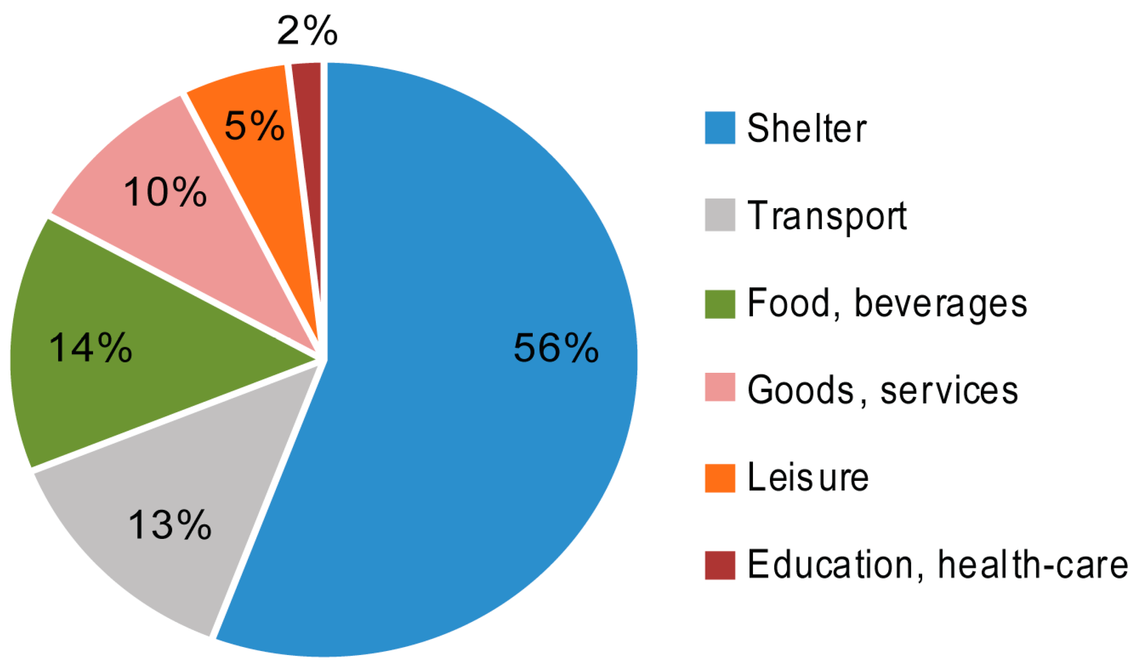
  • Shelter (electricity, heating, water, waste management, maintenance, rent, etc.);
  • Transport (car fuel, purchase and maintenance of vehicles, public transport, flights, etc.);
  • Food and non-alcoholic beverages;
  • Consumer goods and services (clothing, footwear, household equipment, alcohol, tobacco, communication, miscellaneous goods and services);
  • Leisure (recreation, culture, accommodation, restaurants);
  • Education and healthcare.
In the statistical analysis we use analysis of variance (ANOVA) and multiple linear regression modeling. ANOVA in Section 3.2 is undertaken on a per capita basis in order to account for the effect of household size. Multiple regression models in Section 3.3 use per household carbon emissions as the dependent variable and we apply household type as one of the explanatory variables. These models involve only those sociodemographic household characteristics that turned out to be statistically significant (p < 0.05) in the preparatory analysis. Households with zero costs in a particular consumption cluster are omitted from the respective regression model due to the need to transform dependent values logarithmically in order to obtain a normal distribution of the model residuals. As a result, the models of the transport and healthcare and education clusters involve a restricted set of the households, 55% and 51% respectively, while the rest of the consumption clusters represent 90%–100% of the households from the sample.

3. Results

3.1. Carbon Load of Household Consumption in Estonia

The carbon load of final consumption in Estonia in the year 2012 was on average 8.6 t CO2 per household and 3.9 t CO2 per capita, with a 95% confidence interval between 8.5–8.8 t CO2 and 3.8–4.0 t CO2 respectively. The dominant share of per capita emissions was held by shelter (56%, Figure 1) in which domestic energy accounted for the majority of the emissions (52% of total per capita emissions). Among other consumption clusters, the largest share was the consumption of food and non-alcoholic beverages (14%), followed by transport (13%), and the consumption of various consumer goods and services (10%), while other consumption categories constituted lower shares. Direct energy use, i.e., domestic energy and car fuel, accounted for 60% of the emissions.

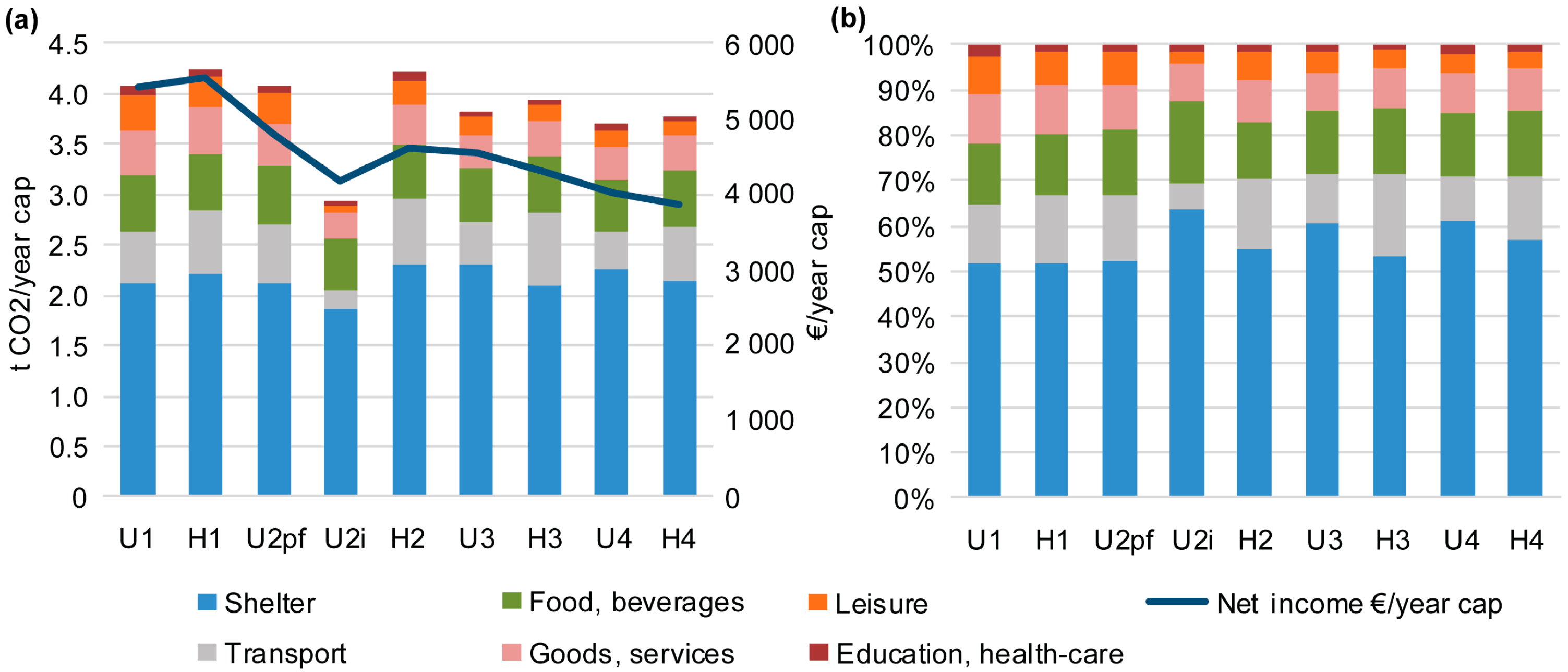
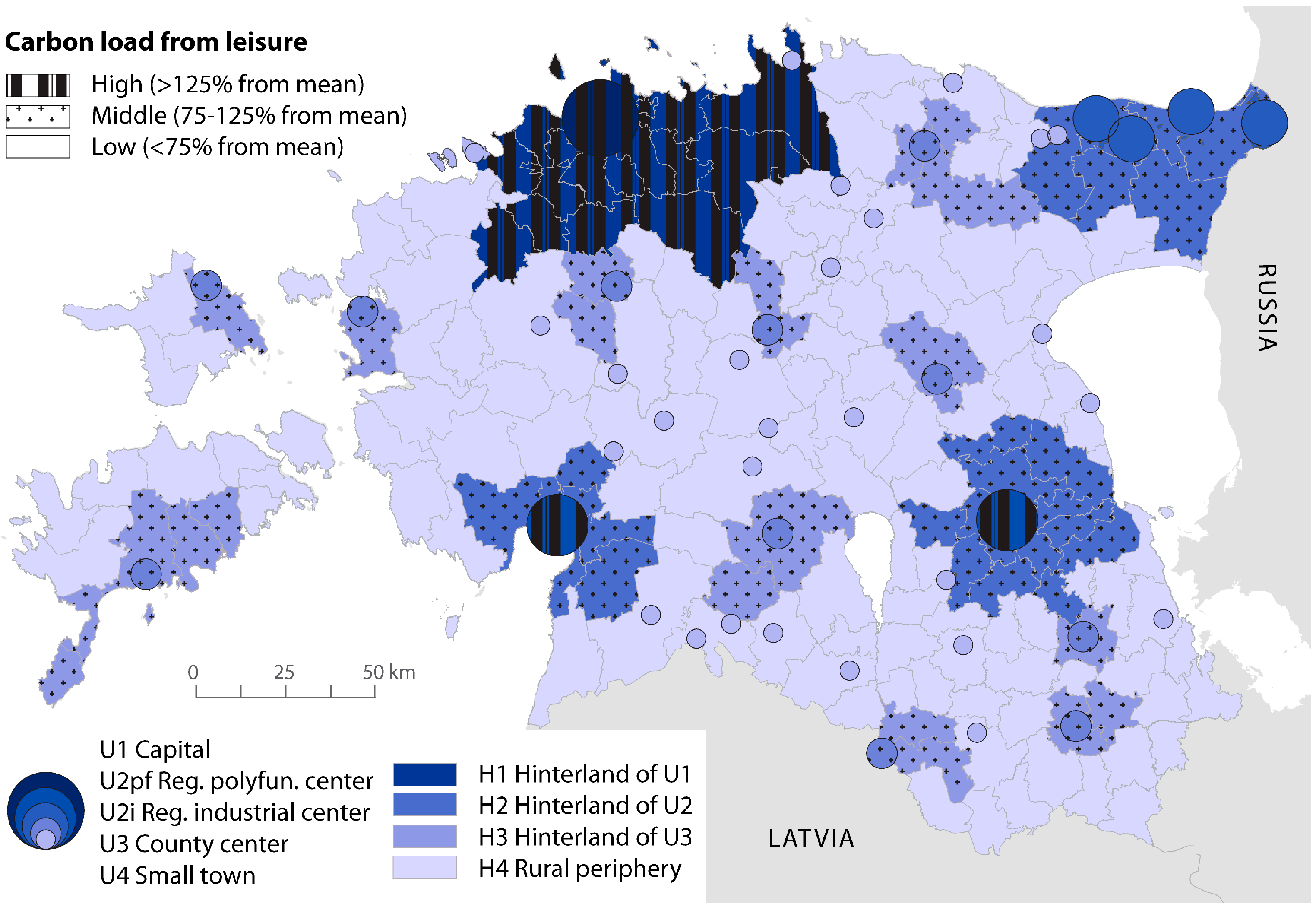
3.2. Differences in per Capita Carbon Load Across Settlement Hierarchy Levels

Per capita carbon emissions of Estonian households tend to be higher among the residents of higher hierarchy levels, i.e., the capital region and regional polyfunctional centers and their hinterlands, than among the residents of lower-level settlement hierarchy levels, i.e., county centers and their hinterlands, small towns, and rural peripheral municipalities (Figure 2a). However, overwhelmingly, the lowest load is shown by the residents of regional industrial centers. On per household level, the carbon emissions are significantly higher (p < 0.001… p < 0.05) among the households of the hinterlands of the capital and regional centers than among households residing in any other settlement hierarchy level, and significantly lower (p < 0.001) among the households residing in regional industrial centers than those residing elsewhere.
There are significant (p < 0.01) differences between the residents of different settlement hierarchy levels in the per capita carbon load of all of the studied consumption clusters, with the exception of the food and beverage cluster and domestic energy use, which accounts for the majority of the emissions within the shelter cluster. As a result, the food and beverage and shelter clusters hold higher shares in the total carbon emissions of the residents of regional industrial centers (Figure 2b). Within the shelter consumption cluster, per capita emissions other than domestic energy decrease steadily from the capital towards lower-level urban cores, and the emissions among the residents from the hinterland are always lower than among those residing in the respective level of the urban core, with the exception of the regional industrial centers.
Per capita transport-related emissions show ambiguous regional disparities. Higher per capita emissions from all transport-related costs are related to residents from the hinterlands of urban centers (Figure S1). Emissions from car fuel are roughly equal across all levels of urban cores (with the exception of regional industrial centers, which contain the lowest values) and significantly (p < 0.05) higher in the hinterland of county centers and rural peripheral municipalities. The average emissions from public transport are in turn higher among the residents of the capital region and regional polyfunctional centers than in lower-level settlement units. Statistically significant difference does not, however, occur between every possible combination of these hierarchy levels. Apart from everyday travel, there are other transport-related costs such as the purchase and maintenance of vehicles and traveling by air or sea. The carbon emissions from these expenditures show a decreasing trend across settlement hierarchy, resulting in statistically significant (p < 0.01) differences between residents of the capital and residents from small towns and rural peripheral municipalities. The dominant part of these emissions stems from vehicle-related costs.
Our results show the largest regional disparities in the case of leisure-related carbon emissions, which follow a significant declining trend from higher towards lower settlement levels, with the exception of the residents of regional industrial centers whose carbon load in this consumption category is significantly (p < 0.01) lower than all other respondents (Figure 3). Diminishing emissions across settlement hierarchy are also reflected in Figure 2a,b. A similar pattern, but with a milder decline across settlement hierarchy, is also present in the carbon emissions of various consumer goods and services (Figure S2).
Carbon emissions from education and healthcare show statistically significant (p < 0.01) differences between residents of the capital on one hand and residents of regional industrial centers, county centers and their hinterland, and rural peripheral municipalities on the other.

3.3. The Carbon Load of Household Consumption and the Impact of Sociodemographic Factors

The spatial variability in the absolute values of carbon emissions of household consumption explored above is a result of a combination of various sociodemographic, economic, and geographic factors as well as individual preferences and social settings. We now examine the impact of these foregoing factors in order to understand the effect of residential location within the settlement hierarchy on the carbon load of households.
The differences in total carbon load of household consumption between settlement hierarchy levels presented in Section 3.2 are primarily explained by socioeconomic factors other than the level of settlement hierarchy as seen from model M1 in Table 3 (adjusted R2 = 0.42). Only households from rural peripheral municipalities show minor statistically significant (p < 0.05) lower emissions than households from the capital. Higher carbon load is related mainly to households with children, higher income, larger living spaces, and the ownership of a private car. In addition, smaller differences occur due to education level, ethnicity, and heating options.
Direct carbon emissions, i.e., emissions from domestic heating and car fuel, do not vary across settlement hierarchy according to our results, and the model (M2 in Table 3) describes only 23% of the variability. However, there are indirect effects related to residential location and land-use characteristics that explain the variance in direct energy emissions. Specifically, higher direct carbon emissions are connected to non-single households who own bigger homes without district heating, who have higher incomes and own a car. Higher carbon emissions from domestic energy use have a weak negative correlation (r = −0.21, p < 0.001) with the presence of district heating.
Significant regional disparities are visible within the consumption categories that cause indirect carbon emissions, where the model (M3 in Table 3) also has the highest ability to describe the variability of the respective emission rates, namely 45%. The highest carbon rates are shown by households living in the hinterland of the capital, differing significantly (p < 0.001) even from households in the capital. At the other end of the scale, households from county centers have the lowest emissions, followed by small towns, peripheral rural municipalities, and regional industrial centers. Income has the overwhelmingly strongest effect on indirect emissions, followed by household type, Estonian as a first language, higher education, larger living space, apartment living, and ownership of a dwelling and a private car.
The exploration of the spatial variability of carbon emissions within single consumption clusters reveals significant differences in every cluster apart from food and non-alcoholic beverages, where the differences in carbon load are explained by households with children, higher per capita income, higher education level, larger living space, dwelling ownership, and living in detached houses (M4 in Table 3, adjusted R2 = 0.29). We do not consider further the emissions of education and healthcare as the model describes only 6% of the variability and covers only 51% of the respondents who declared respective costs.
Considering shelter-related carbon emissions, there are significant (p < 0.01) differences between residents of the capital and residents of lower-level rural municipalities (M5 in Table 3, adjusted R2 = 0.14). Larger living spaces, not having district heating, children in the household, and higher income explain the majority of the variability.
Within transport-related carbon emissions, significant differences (p < 0.01) occur between households of the capital and household of the hinterland of regional centers (M6 in Table 3, adjusted R2 = 0.18). Households who own a car, have a higher income, speak Estonian as a first language, and live in large apartment buildings tend to have higher transport emissions.
The carbon load from the consumption of consumer goods and services is the lowest among households residing in regional industrial centers or in county centers, showing significant (p < 0.001 and 0.05, respectively) differences from the households in the capital (M7 in Table 3, adjusted R2 = 0.36). In addition, households with children, higher per capita income, private cars, higher education, and Estonian as a first language have significantly (p < 0.001) higher carbon load within this consumption cluster. Larger living spaces and living in apartment buildings also favor higher consumption of consumer goods and services.
Among all analyzed consumption clusters, the carbon load from leisure-related goods and services varies the most according to settlement hierarchy (M8 in Table 3, adjusted R2 = 0.31). Households from the hinterland of the capital have the highest carbon load for leisure-related goods and services, showing significant (p < 0.01) differences from households in the capital. The latter, in turn, tend to emit more carbon than households in regional industrial centers and county centers (p < 0.01) or small towns and rural peripheral municipalities (p < 0.001). In addition, higher income, children in the household, Estonian as first language, car ownership, and larger living spaces are all associated with a higher carbon load from leisure-related goods and services.

4. Discussion

We studied the associations between residential location within settlement hierarchies and the carbon load of household consumption. We found that significant spatial variations in carbon load derive from consumption clusters related to welfare and lifestyle, because households from higher hierarchy levels tend to spend more on these goods and services than residents from lower hierarchy levels, even when sociodemographic and economic background is taken into account. Our results are in line with the notion that the presence or absence of consumption spaces and places in the everyday environment affects consumption practices by enabling, predisposing or hindering related forms of consumption ([5] (p. 7); [6] (p. 13)). Consumer and leisure-related resources are more available in higher-level cities and indeed the presence of a multitude of functions is one of the basic characteristics that distinguishes higher hierarchy level settlements from lower ones [12]. Residents are able to engage in a wider set of activities in these higher-level settlements, and their options include spending on hobbies, attending various cultural events, dining out, buying a takeaway coffee, or spending in retail spaces. They are therefore able to express freedom of choice in the context of an abundance of goods [8]. The spatial availability of consumer spaces, together with their visual-cultural environment aiming to persuade people to spend more [7] (p. 151), influence expenditure choices and consequently increase the environmental load imposed by residents from higher hierarchy levels. Significant increases in the purchase of services, but not necessarily tangible goods, along with urbanization featuring equalized income levels have been illustrated in earlier research [52,63].
Our results are the first to uncover the environmental load of household consumption in a Central and Eastern European country. The total annual per capita carbon emission found in the current study was 3.9 t CO2 in 2012, which is 1.2–2.7 times lower than previously found in several other European countries with higher affluence level (see, e.g., [51,59,67,72,105]). The carbon load depends on the total consumption volume of Estonian households and the energy mix used in the country, including the dominant position of oil-shale electricity production. In 2010, mean consumption expenditure by household in Estonia formed about one-third of the average figure of the present 28 countries of the European Union [106], explaining the lower level of our results.
The current study has shown that domestic energy use is the single most important source of carbon emission in Estonian households. This indicates not only the need to look over the general policy of energy sources or to improve the current state of energy efficiency in the housing stock in Estonia as a country with a Nordic climate (as is also stipulated by the national energy roadmap) [82], but also the need to better integrate climate change mitigation issues within spatial planning practices [50]. Although our results reveal no significant spatial differences in domestic energy use between settlement hierarchy levels, geographic distinctions emerge due to the presence of district heating that tends to lower the carbon emissions of domestic energy use. This is in line with the common understanding of the favorable role that district heating can play in achieving energy-efficiency goals [30,56]. Dwelling-related emissions other than domestic energy differ across settlement hierarchy because urban housing estates more commonly involve commercial maintenance and water treatment services while households in traditional rural environments rely more on owner-related maintenance and local non-commercial water supplies and treatments.
Our results affirm the car-dependency of people residing outside urban cores, which is a result of suburbanization processes together with the decline in public transport provision outside cities [77]. Nevertheless, total transport carbon load in absolute terms is still higher in the capital region and regional polyfunctional centers. This is probably a result of longer inner-city distances [10,36] in combination with higher affluence levels and greater proximity to commercial welfare- and leisure-related activities that may induce further travel. Our results show that life in regional industrial centers, county centers, and small towns is the most resource-saving because these residents need less motorized transport to reach their everyday destinations. Therefore, there is a need to improve the usability of light transport modes in urban centers and apply more rigorous principles regarding the importance of public transport connectivity in the development of new suburban areas. Spatial planning policy is the means by which this can be achieved and this therefore plays key role in the transition of urban transport energy use, alongside sociodemographic, psychological, and institutional factors [41].
The low carbon load of households residing in regional industrial centers is only partly explained by economic or demographic characteristics. The industrial and ethnic background of those settlements, in housing dominated by Soviet-era apartment blocks, below-national-average income level, and Soviet-era legacies in consumption culture and mentality have probably hindered these centers from developing into postmodern hubs of consumption and leisure, even though their size and regional importance could enable more economic activities and opportunities for consumer culture. Research from the capital region has shown that non-Estonians have a smaller non-employment-related out-of-capital activity space than Estonians, referring to some spatial segregation of leisure activities along ethnic lines [107]. Other authors have shown that market-based consumer culture ‘is the most neutral, non-discriminating and accessible area where Estonian Russians’ feeling of exclusion is alleviated’ [108] (p. 68). The young Russian-speaking minorities seem to be especially affected by transnational media and consumer culture because they have a stronger consumerist orientation, including in the form of window-shopping, than their Estonian peers [108]. Among elderly groups, who also form the majority of Russian speakers in Estonia, this orientation is absent [108], and elderly groups are more prone to continue the practices of the conservative consumer culture of the Soviet era, characterized by shortages and homogeneity [109].
We are aware that residential and lifestyle preferences are interconnected and may explain some of the spatial differences in consumption patterns and consequent carbon emissions. Research on residential selection has acknowledged that people, from within their life-course- and employment-related constraints, choose a living environment that suits their preferences regarding neighborhood characteristics [110], travel attitudes [111,112], household energy consumption [113], or recreational and cultural amenities [114,115]. For example, it has been shown that the metropolitan core with its rich opportunities for culture, entertainment, and sport activities attracts knowledge-workers with culture-oriented lifestyles, while home-oriented people tend to choose suburban living environments [116]. In Estonia, out-migration from rural areas is related to employment, self-realization, and the avoidance of marginalization [80]. We may assume that the capital region attracts people with an active lifestyle. Our data do not allow us to test the hypothesis of residential self-selection, hence this requires further scholarly attention.

5. Conclusions

Residential location in settlement hierarchy frames the environmental load of consumption and mobility. In equal conditions of affluence and other socio-demographic variables of households, the location of home in settlement hierarchy significantly influences the carbon load of consumption clusters that are especially related to welfare and lifestyle. The current study has several limitations regarding the methodology of input-output computing related to the aggregation errors [88,94] and the limited choice of indicators when describing the environmental load of household consumption as described in Section 2.3. At the same time, it is the first to cover the spatial dimension in the environmental load of household expenditure among the entire Estonian population, revealing significant spatial differences especially in the field of indirect consumption, which have not previously attracted sufficient scholarly attention. There is a need to combine quantitative results from expenditure surveys with social network and activity studies of the populations of different settlement types in order to capture the interrelated character of choices in the material, social, and cultural settings of the everyday environment. Integrated spatial planning policy that takes into account transport, energy use, production, and consumption practices is needed on local, regional, national, and international levels in order to support and achieve socially, economically, and environmentally balanced ways of living.

Supplementary Materials

The following are available online at www.mdpi.com/2071-1050/8/9/799/s1, Figure S1: The spatial patterns of relative per capita carbon load from transport in comparison to mean carbon load across settlement hierarchy levels, Figure S2: The spatial patterns of relative per capita carbon load from consumer goods and services in comparison to mean carbon load across settlement hierarchy levels, Table S1: Emission intensities of various consumption categories used in the analysis.

Acknowledgments

This research has been supported by the Institutional Research Grant No. IUT2-17 of Estonian Research Agency, co-funded by European Union Horizon 2020 action Smart Cities and Communities (SCC-2015) project SmartEnCity (Gran Agreement 691883), and the national scholarship program Kristjan Jaak, which is funded and managed by the Archimedes Foundation in collaboration with the Ministry of Education and Research.

Author Contributions

Age Poom was the primary author of the manuscript, conceived and designed the research, analyzed the data, prepared the maps, and wrote the paper. Rein Ahas contributed with the general organization and coordination of the work process and the paper, the interpretation of the results and the elaboration of the discussion, in addition to final review of the manuscript.

Conflicts of Interest

The authors declare no conflict of interest.

References

  1. United Nations. Spatial Planning: Key Instruments for Development and Effective Governance with Special Reference to Countries in Transition; United Nations Economic Commission for Europe: Geneva, Switzerland, 2008; p. 46. [Google Scholar]
  2. European Commission. ESDP: European Spatial Development Perspective towards Balanced and Sustainable Development of the Territory; European Commission—Committee on Spatial Development: Luxembourg, Luxembourg, 1999; p. 87. [Google Scholar]
  3. Hertwich, E.G.; Peters, G.P. Carbon footprint of nations: A global, trade-linked analysis. Environ. Sci. Technol. 2009, 43, 6414–6420. [Google Scholar] [CrossRef] [PubMed]
  4. Dodman, D. Blaming cities for climate change? An analysis of urban greenhouse gas emissions inventories. Environ. Urban 2009, 21, 185–201. [Google Scholar] [CrossRef]
  5. Smas, L. Konsumtion, det Urbana Livet och Stadens Morfologi [Consumption, Urban Life, and the Morphology of Cities]. In Transaktioner ur ett Tidrumsligt Perspektiv [Transactions from a Space-Time Perspective]. Kulturgeografiskt Seminarium 1. Rapporter/Meddelanden/Uppsatter Fran Kulturgeografiska Institutionen; University of Stockholm: Stockholm, Sweden, 2005. [Google Scholar]
  6. Goodman, M.K.; Goodman, D.; Redclift, M. Introduction: Situating Consumption, Space and Place. In Consuming Space: Placing Consumption in Perspective; Goodman, M.K., Goodman, D., Redclift, M., Eds.; Ashgate: Farnham, UK, 2010; pp. 3–40. [Google Scholar]
  7. Hudson, R. Economic Geographies: Circuits, Flows and Spaces; SAGE Publications: London, UK; Thousand Oaks, CA, USA; New Delhi, India, 2005; p. 248. [Google Scholar]
  8. Keller, M. Representations of Consumer Culture in Post-Soviet Estonia: Transformations and Tensions. Ph.D. Thesis, University of Tartu, Tartu, Estonia, 2004. [Google Scholar]
  9. Christaller, W. Die Zentralen Orte in Süddeutschland; Gustav Fischer: Jena, Germany, 1933. [Google Scholar]
  10. Poom, A.; Ahas, R.; Orru, K. The impact of residential location and settlement hierarchy on ecological footprint. Environ. Plan. A 2014, 46, 2369–2384. [Google Scholar] [CrossRef]
  11. Lenzen, M.; Wier, M.; Cohen, C.; Hayami, H.; Pachauri, S.; Schaeffer, R. A comparative multivariate analysis of household energy requirements in Australia, Brazil, Denmark, India and Japan. Energy 2006, 31, 181–207. [Google Scholar] [CrossRef]
  12. Berry, B.J.L. Shopping Centers and the Geography of Urban Areas. A Theoretical and Empirical Study of the Spatial Structure of Intraurban Retail and Service Business. Ph.D. Thesis, University of Washington, Seattle, DC, USA, 1958. [Google Scholar]
  13. Burgalassi, D.; Luzzati, T. Urban spatial structure and environmental emissions: A survey of the literature and some empirical evidence for Italian NUTS 3 regions. Cities 2015, 49, 134–148. [Google Scholar] [CrossRef]
  14. Jorgenson, A.K.; Burns, T.J. The political-economic causes of change in the ecological footprints of nations, 1991–2001: A quantitative investigation. Soc. Sci. Res. 2007, 36, 834–853. [Google Scholar] [CrossRef]
  15. Heinonen, J.; Kyrö, R.; Junnila, S. Dense downtown living more carbon intense due to higher consumption: A case study of Helsinki. Environ. Res. Lett. 2011. [Google Scholar] [CrossRef]
  16. Wiedenhofer, D.; Lenzen, M.; Steinberger, J.K. Energy requirements of consumption: Urban form, climatic and socio-economic factors, rebounds and their policy implications. Energy Policy 2013, 63, 696–707. [Google Scholar] [CrossRef]
  17. Chua, B.-H. World cities, globalisation and the spread of consumerism: A view from Singapore. Urban Stud. 1998, 35, 981–1000. [Google Scholar] [CrossRef]
  18. Gregory, D.; Johnston, R.; Pratt, G.; Watts, M.; Whatmore, S. The Dictionary of Human Geography, 5th ed; Wiley-Blackwell: Chichester, UK, 2009. [Google Scholar]
  19. Guy, C.M. Controlling new retail spaces: The impress of planning policies in Western Europe. Urban Stud. 1998, 35, 953–979. [Google Scholar] [CrossRef]
  20. Di Donato, M.; Lomas, P.L.; Carpintero, Ó. Metabolism and environmental impacts of household consumption: A review on the assessment, methodology, and drivers. J. Ind. Ecol. 2015, 19, 904–916. [Google Scholar] [CrossRef]
  21. Noorman, K.J.; Biesiot, W.; Schoot Uiterkamp, A.J.M. Household Metabolism in the Context of Sustainability and Environmental Quality. In Green Households? Domestic Consumers, Environment, and Sustainability; Noorman, K.J., Schoot Uiterkamp, A.J.M., Eds.; Earthscan: London, UK, 1998; pp. 7–34. [Google Scholar]
  22. Druckman, A.; Sinclair, P.; Jackson, T. A geographically and socio-economically disaggregated local household consumption model for the UK. J. Clean. Prod. 2008, 16, 870–880. [Google Scholar] [CrossRef] [Green Version]
  23. Moll, H.C.; Noorman, K.J.; Kok, R.; Engström, R.; Throne-Holst, H.; Clark, C. Pursuing more sustainable consumption by analyzing household metabolism in European countries and cities. J. Ind. Ecol. 2005, 9, 259–275. [Google Scholar] [CrossRef] [Green Version]
  24. Kerkhof, A.C.; Nonhebel, S.; Moll, H.C. Relating the environmental impact of consumption to household expenditures: An input-output analysis. Ecol. Econ. 2009, 68, 1160–1170. [Google Scholar] [CrossRef]
  25. Herendeen, R.A. Total energy cost of household consumption in Norway, 1973. Energy 1978, 3, 615–630. [Google Scholar] [CrossRef]
  26. Herendeen, R.A.; Ford, C.; Hannon, B. Energy cost of living, 1972–1973. Energy 1981, 6, 1433–1450. [Google Scholar] [CrossRef]
  27. Muñiz, I.; Galindo, A. Urban form and the ecological footprint of commuting. The case of Barcelona. Ecol. Econ. 2005, 55, 499–514. [Google Scholar]
  28. Newman, P.W.G.; Kenworthy, J.R. Gasoline consumption and cities. A comparison of U.S. cities with a global survey. J. Am. Plan. Assoc. 1989, 55, 24–37. [Google Scholar] [CrossRef]
  29. Larson, W.; Liu, F.; Yezer, A. Energy footprint of the city: Effects of urban land use and transportation policies. J. Urban Econ. 2012, 72, 147–159. [Google Scholar] [CrossRef]
  30. Holden, E.; Norland, I.T. Three challenges for the compact city as a sustainable urban form: Household consumption of energy and transport in eight residential areas in the Greater Oslo Region. Urban Stud. 2005, 42, 2145–2166. [Google Scholar] [CrossRef]
  31. Ewing, R.; Rong, F. The impact of urban form on U.S. residential energy use. Hous. Policy Debate 2008, 19, 1–30. [Google Scholar] [CrossRef]
  32. Brown, M.A.; Southworth, F.; Sarzynski, A. The geography of metropolitan carbon footprints. Policy Soc. 2009, 27, 285–304. [Google Scholar] [CrossRef]
  33. Næss, P.; Vogel, N. Sustainable urban development and the multi-level transition perspective. Environ. Innov. Soc. Trans. 2012, 4, 36–50. [Google Scholar] [CrossRef]
  34. Lefèvre, B. Urban transport energy consumption: Determinants and strategies for its reduction. An analysis of the literature. Sapiens 2009, 2, 1–17. [Google Scholar]
  35. Ewing, R.; Cervero, R. Travel and the built environment. J. Am. Plan. Assoc. 2010, 76, 265–294. [Google Scholar] [CrossRef]
  36. Stead, D.; Marshall, S. The relationships between urban form and travel patterns. An international review and evaluation. Eur. J. Transp. Infrastruct. Res. 2001, 1, 113–141. [Google Scholar]
  37. Cao, X.; Mokhtarian, P.L.; Handy, S.L. The relationship between the built environment and nonwork travel: A case study of Northern California. Transp. Res. A Pol. 2009, 43, 548–559. [Google Scholar] [CrossRef]
  38. Jones, C.; Kammen, D.M. Spatial distribution of U.S. household carbon footprints reveals suburbanization undermines greenhouse gas benefits of urban population density. Environ. Sci. Technol. 2013, 48, 895–902. [Google Scholar] [CrossRef] [PubMed]
  39. Rodriguez, D.A.; Targa, F.; Aytur, S.A. Transport Implications of urban containment policies: A study of the largest twenty-five US metropolitan areas. Urban Stud. 2006, 43, 1879–1897. [Google Scholar] [CrossRef]
  40. Stead, D. Relationships between land use, socioeconomic factors, and travel patterns in Britain. Environ. Plan. B 2001, 28, 499–528. [Google Scholar] [CrossRef]
  41. Zhao, P.; Pendlebury, J. Spatial planning and transport energy transition towards a low carbon system. disP Plan. Rev. 2014, 50, 20–30. [Google Scholar] [CrossRef]
  42. Rickwood, P.; Glazebrook, G.; Searle, G. Urban structure and energy—A review. Urban Policy Res. 2008, 26, 57–81. [Google Scholar] [CrossRef]
  43. Heinonen, J.; Junnila, S. Residential energy consumption patterns and the overall housing energy requirements of urban and rural households in Finland. Energy Build. 2014, 76, 295–303. [Google Scholar] [CrossRef]
  44. Kaza, N. Understanding the spectrum of residential energy consumption: A quantile regression approach. Energy Policy 2010, 38, 6574–6585. [Google Scholar] [CrossRef]
  45. Estiri, H. Household energy consumption and housing choice in the U.S. residential sector. Hous. Policy Debate 2016, 26, 231–250. [Google Scholar] [CrossRef]
  46. Estiri, H. The indirect role of households in shaping US residential energy demand patterns. Energy Policy 2015, 86, 585–594. [Google Scholar] [CrossRef]
  47. Guerra Santin, O.; Itard, L.; Visscher, H. The effect of occupancy and building characteristics on energy use for space and water heating in Dutch residential stock. Energy Build. 2009, 41, 1223–1232. [Google Scholar] [CrossRef]
  48. Kuzyk, L.W. The ecological footprint housing component: A geographic information system analysis. Ecol. Indic. 2012, 16, 31–39. [Google Scholar] [CrossRef]
  49. Glaeser, E.L.; Kahn, M.E. The greenness of cities: Carbon dioxide emissions and urban development. J. Urban Econ. 2010, 67, 404–418. [Google Scholar] [CrossRef]
  50. Wende, W.; Huelsmann, W.; Marty, M.; Penn-Bressel, G.; Bobylev, N. Climate protection and compact urban structures in spatial planning and local construction plans in Germany. Land Use Policy 2010, 27, 864–868. [Google Scholar] [CrossRef]
  51. Ottelin, J.; Heinonen, J.; Junnila, S. New energy efficient housing has reduced carbon footprints in outer but not in inner urban areas. Environ. Sci. Technol. 2015, 49, 9574–9583. [Google Scholar] [CrossRef] [PubMed]
  52. Heinonen, J.; Jalas, M.; Juntunen, J.K.; Ala-Mantila, S.; Junnila, S. Situated lifestyles: II. The impacts of urban density, housing type and motorization on the greenhouse gas emissions of the middle-income consumers in Finland. Environ. Res. Lett. 2013. [Google Scholar] [CrossRef]
  53. O’Regan, B.; Morrissey, J.; Foley, W.; Moles, R. The relationship between settlement population size and sustainable development measured by two sustainability metrics. Environ. Impact Assess. 2009, 29, 169–178. [Google Scholar] [CrossRef]
  54. Slagstad, H.; Brattebo, H. LCA for household waste management when planning a new urban settlement. Waste Manag. 2012, 32, 1482–1490. [Google Scholar] [CrossRef] [PubMed]
  55. Põldnurk, J. Optimisation of the economic, environmental and administrative efficiency of the municipal waste management model in rural areas. Resour. Conserv. Recycl. 2015, 97, 55–65. [Google Scholar] [CrossRef]
  56. Connolly, D.; Lund, H.; Mathiesen, B.V.; Werner, S.; Möller, B.; Persson, U.; Boermans, T.; Trier, D.; Østergaard, P.A.; Nielsen, S. Heat roadmap Europe: Combining district heating with heat savings to decarbonise the EU energy system. Energy Policy 2014, 65, 475–489. [Google Scholar] [CrossRef]
  57. Ristimäki, M.; Säynäjoki, A.; Heinonen, J.; Junnila, S. Combining life cycle costing and life cycle assessment for an analysis of a new residential district energy system design. Energy 2013, 63, 168–179. [Google Scholar] [CrossRef]
  58. Anker-Nilssen, P. Household energy use and the environment—A conflicting issue. Appl. Energy 2003, 76, 189–196. [Google Scholar] [CrossRef]
  59. Kerkhof, A.C.; Benders, R.M.J.; Moll, H.C. Determinants of variation in household CO2 emissions between and within countries. Energy Policy 2009, 37, 1509–1517. [Google Scholar] [CrossRef]
  60. Weber, C.L.; Matthews, H.S. Quantifying the global and distributional aspects of American household carbon footprint. Ecol. Econ. 2008, 66, 379–391. [Google Scholar] [CrossRef]
  61. Baiocchi, G.; Minx, J.; Hubacek, K. The impact of social factors and consumer behavior on carbon dioxide emissions in the United Kingdom. J. Ind. Ecol. 2010, 14, 50–72. [Google Scholar] [CrossRef]
  62. Tammaru, T.; Musterd, S.; van Ham, M.; Marcinczak, S. A Multi-Factor Approach to Understanding Socio-Economic Segregation in European Capital Cities. In Socio-Economic Segregation in European Capital Cities. East Meast West; Tammaru, T., Marcinczak, S., van Ham, M., Musterd, S., Eds.; Routledge: London, UK; New York, NY, USA, 2016; pp. 1–29. [Google Scholar]
  63. Ala-Mantila, S.; Heinonen, J.; Junnila, S. Relationship between urbanization, direct and indirect greenhouse gas emissions, and expenditures: A multivariate analysis. Ecol. Econ. 2014, 104, 129–139. [Google Scholar] [CrossRef]
  64. Tukker, A.; Jansen, B. Environmental impacts of products: A detailed review of studies. J. Ind. Ecol. 2006, 10, 159–182. [Google Scholar] [CrossRef]
  65. Sánchez-Chóliz, J.; Duarte, R.; Mainar, A. Environmental impact of household activity in Spain. Ecol. Econ. 2007, 62, 308–318. [Google Scholar] [CrossRef]
  66. Wier, M.; Lenzen, M.; Munksgaard, J.; Smed, S. Effects of household consumption patterns on CO2 requirements. Econ. Syst. Res. 2001, 13, 259–274. [Google Scholar] [CrossRef]
  67. Heinonen, J.; Junnila, S. A carbon consumption comparison of rural and urban lifestyles. Sustainability 2011, 3, 1234–1249. [Google Scholar] [CrossRef]
  68. Heinonen, J.; Junnila, S. Implications of urban structure on carbon consumption in metropolitan areas. Environ. Res. Lett. 2011. [Google Scholar] [CrossRef]
  69. Heinonen, J.; Jalas, M.; Juntunen, J.K.; Ala-Mantila, S.; Junnila, S. Situated lifestyles: I. How lifestyles change along with the level of urbanization and what the greenhouse gas implications are—A study of Finland. Environ. Res. Lett. 2013. [Google Scholar] [CrossRef]
  70. Shammin, M.R.; Herendeen, R.A.; Hanson, M.J.; Wilson, E.J.H. A multivariate analysis of the energy intensity of sprawl versus compact living in the U.S. for 2003. Ecol. Econ. 2010, 69, 2363–2373. [Google Scholar] [CrossRef]
  71. Druckman, A.; Jackson, T. The carbon footprint of UK households 1990–2004: A socio-economically disaggregated, quasi-multi-regional input–output model. Ecol. Econ. 2009, 68, 2066–2077. [Google Scholar] [CrossRef] [Green Version]
  72. Büchs, M.; Schnepf, S.V. Who emits most? Associations between socio-economic factors and UK households’ home energy, transport, indirect and total CO2 emissions. Ecol. Econ. 2013, 90, 114–123. [Google Scholar]
  73. Marksoo, A. Tallinn Eesti rahvarände süsteemis [Tallinn in the Estonian migration system]. In Eesti Geograafia Seltsi Aastaraamat [Yearbook of Estonian Geographic Society]; Raukas, A., Jõgi, J., Marksoo, A., Punning, M., Tarand, A., Eds.; Valgus: Tallinn, Estonia, 1990; Volume 25, pp. 53–66. [Google Scholar]
  74. Tammaru, T.; Kulu, H.; Kask, I. Siserände üldsuunad [Trends in internal migration]. In Ränne üleminekuaja Eestis [Migration in transitional Estonia]; Tammaru, T., Kulu, H., Eds.; Statistics Estonia: Tallinn, Estonia, 2003; pp. 5–27. [Google Scholar]
  75. Marksoo, A. On the development concept of small towns in the Estonian SSR. In Estonia: Geographical Researches; Punning, J.-M., Ed.; Academy of Sciences of the Estonian SSR, Estonian Geographical Society: Tallinn, Estonia, 1980; pp. 110–126. [Google Scholar]
  76. Marksoo, A. Regularities of Urbanization and Demographical Processes in the Estonian SSR. In Problems of Territorial Organization of Geographical Systems; Mardiste, H., Marksoo, A., Eds.; Tartu State University: Tartu, Estonia, 1984; pp. 32–56. [Google Scholar]
  77. Statistics Estonia. Statistical Databases: Economy and Social Life. Available online: http://pub.stat.ee/px-web.2001/dialog/statfile1.asp (accessed on 22 Feberary 2016).
  78. Ministry of Economic Affairs and Communications. Transpordi Arengukava 2014–2020 [Estonian Transportation Roadmap 2014–2020]; Ministry of Economic Affairs and Communications: Tallinn, Estonia, 2013; p. 70.
  79. Tiit, E.-M.; Servinski, M. Eesti Maakondade Rahvastik: Hinnatud ja Loendatud [Population of Estonian Counties: Estimated and Counted]; Statistikaamet: Tallinn, Estonia, 2015; p. 420. [Google Scholar]
  80. Nugin, R. I think that they should go. Let them see something. The context of rural youth’s out-migration in post-socialist Estonia. J. Rural Stud. 2014, 34, 51–64. [Google Scholar] [CrossRef]
  81. EEA. Resource-Efficient Green Economy and EU Policies; European Environmental Agency, Publications Office of the European Union: Luxembourg City, Luxembourg, 2014; p. 107. [Google Scholar]
  82. Ministry of Economic Affairs and Communications. ENMAK 2030+ Eesti Energiamajanduse Arengukava Aastani 2030 [Estonian Energy Roadmap 2030+]; Ministry of Economic Affairs and Communications: Tallinn, Estonia, 2015.
  83. Kurnitski, J.; Kuusk, K.; Tark, T.; Uutar, A.; Kalamees, T.; Pikas, E. Energy and investment intensity of integrated renovation and 2030 cost optimal savings. Energy Build. 2014, 75, 51–59. [Google Scholar] [CrossRef]
  84. Statistics Estonia. Statistical Databases: Economy. Available online: http://pub.stat.ee/px-web.2001/dialog/statfile1.asp (accessed on 5 January 2015).
  85. Ministry of Economic Affairs and Communications. ENMAK 2020 Energiamajanduse Riiklik Arengukava Aastani 2020. (Energy Roadmap 2020); Ministry of Economic Affairs and Communications: Tallinn, Estonia, 2009.
  86. United Nations. COICOP: Classification of Individual Consumption According to Purpose. Available online: http://unstats.un.org/unsd/cr/registry/regcst.asp?Cl=5 (accessed on 5 January 2015).
  87. Statistics Estonia. Leibkonna Eelarve Uuring 2010. Metoodika. Household Budget Survey 2010. Methodology; Statistics Estonia: Tallinn, Estonia, 2012; p. 76.
  88. Bicknell, K.B.; Ball, R.J.; Cullen, R.; Bigsby, H.R. New methodology for the ecological footprint with an application to the New Zealand economy. Ecol. Econ. 1998, 27, 149–160. [Google Scholar] [CrossRef]
  89. Leontief, W. Input-Output Economics; Oxford University Press: Oxford, UK, 1986. [Google Scholar]
  90. Leontief, W. The Structure of American Economy, 1919–1929: An Empirical Application of Equilibrium Analysis; Harvard University Press: Cambridge, UK, 1941. [Google Scholar]
  91. Hertwich, E.G. The life cycle environmental impacts of consumption. Econ. Syst. Res. 2011, 23, 27–47. [Google Scholar] [CrossRef]
  92. Minx, J.C.; Wiedmann, T.; Wood, R.; Peters, G.P.; Lenzen, M.; Owen, A.; Scott, K.; Barrett, J.; Hubacek, K.; Baiocchi, G.; et al. Input–output analysis and carbon footprinting: An overview of applications. Econ. Syst. Res. 2009, 21, 187–216. [Google Scholar] [CrossRef]
  93. Ferng, J.-J. Using composition of land multiplier to estimate ecological footprints associated with production activity. Ecol. Econ. 2001, 37, 159–172. [Google Scholar] [CrossRef]
  94. Cellura, M.; Longo, S.; Mistretta, M. The energy and environmental impacts of Italian households consumptions: An input-output approach. Renew. Sustain. Energy Rev. 2011, 15, 3897–3908. [Google Scholar] [CrossRef]
  95. Suh, S.; Lenzen, M.; Treloar, G.J.; Hondo, H.; Horvath, A.; Huppes, G.; Jolliet, O.; Klann, U.; Krewitt, W.; Moriguchi, Y.; et al. System boundary selection in life-cycle inventories using hybrid approaches. Environ. Sci. Technol. 2004, 38, 657–664. [Google Scholar] [CrossRef] [PubMed]
  96. Weinzettel, J.; Steen-Olsen, K.; Hertwich, E.G.; Borucke, M.; Galli, A. Ecological footprint of nations: Comparison of process analysis, and standard and hybrid multiregional input-output analysis. Ecol. Econ. 2014, 101, 115–126. [Google Scholar] [CrossRef]
  97. Nijdam, D.S.; Wilting, H.C.; Goedkoop, M.J.; Madsen, J. Environmental load from Dutch private consumption: How much damage takes place abroad? J. Ind. Ecol. 2005, 9, 147–168. [Google Scholar] [CrossRef]
  98. Kok, R.; Benders, R.M.J.; Moll, H.C. Measuring the environmental load of household consumption using some methods based on input-output energy analysis: A comparison of methods and a discussion of results. Energy Policy 2006, 34, 2744–2761. [Google Scholar] [CrossRef]
  99. Tukker, A.; Poliakov, E.; Heijungs, R.; Hawkins, T.; Neuwahl, F.; Rueda-Cantuche, J.M.; Giljum, S.; Moll, S.; Oosterhaven, J.; Bouwmeester, M. Towards a global multi-regional environmentally extended input-output database. Ecol. Econ. 2009, 68, 1928–1937. [Google Scholar] [CrossRef]
  100. Xu, Y.; Dietzenbacher, E. A structural decomposition analysis of the emissions embodied in trade. Ecol. Econ. 2014, 101, 10–20. [Google Scholar] [CrossRef]
  101. Timmer, M.P.; Dietzenbacher, E.; Los, B.; Stehrer, R.; de Vries, G.J. An illustrated user guide to the world input-output database: The case of global automotive production. Rev. Int. Econ. 2015, 23, 575–605. [Google Scholar] [CrossRef]
  102. Ministry of the Environment. Greenhouse Gas Emissions in Estonia 1990–2012: National Inventory Report under the UNFCCC and the Kyoto Protocol; Ministry of the Environment: Tallinn, Estonia, 2014; p. 335.
  103. Eurostat. Metadata. Statistical Classification of Products by Activity in the European Economic Community, 2008 Version. Available online: http://ec.europa.eu/eurostat/ramon/nomenclatures/index.cfm?TargetUrl=LST_NOM_DTL&StrNom=CPA_2008&StrLanguageCode=EN&IntPcKey=&StrLayoutCode=HIERARCHIC (accessed on 5 January 2015).
  104. Eurostat. Correspondence Table COICOP 1999—CPA 2008; Eurostat: Luxembourg, Luxembourg, 2012; p. 134. [Google Scholar]
  105. Girod, B.; De Haan, P. More or Better? A Model for Changes in Household Greenhouse Gas Emissions due to Higher Income. J. Ind. Ecol. 2010, 14, 31–49. [Google Scholar] [CrossRef]
  106. Eurostat. The Database of Household Budget Surveys. Available online: http://ec.europa.eu/eurostat/web/household-budget-surveys/database (accessed on 18 July 2016).
  107. Silm, S.; Ahas, R. Ethnic differences in activity spaces: A study of out-of-home nonemployment activities with mobile phone data. Ann. Assoc. Am. Geogr. 2014, 104, 542–559. [Google Scholar] [CrossRef]
  108. Kalmus, V.; Keller, M.; Kiisel, M. Emerging consumer types in a transition culture: Consumption patterns of generational and ethnic groups in Estonia. J. Balt Stud. 2009, 40, 53–74. [Google Scholar] [CrossRef]
  109. Keller, M.; Vihalemm, T. Coping with consumer culture: Elderly urban consumers in post-Soviet Estonia. Trames 2005, 9, 69–91. [Google Scholar]
  110. Kährik, A.; Leetmaa, K.; Tammaru, T. Residential decision-making and satisfaction among new suburbanites in the Tallinn urban region, Estonia. Cities 2012, 29, 49–58. [Google Scholar] [CrossRef]
  111. Mokhtarian, P.L.; Cao, X. Examining the impacts of residential self-selection on travel behavior: A focus on methodologies. Transp. Res. B Meth. 2008, 42, 204–228. [Google Scholar] [CrossRef]
  112. De Vos, J.; Witlox, F. Do people live in urban neighbourhoods because they do not like to travel? Analysing an alternative residential self-selection hypothesis. Travel Behav. Soc. 2016, 4, 29–39. [Google Scholar] [CrossRef]
  113. Biying, Y.; Zhang, J.; Fujiwara, A. Analysis of the residential location choice and household energy consumption behavior by incorporating multiple self-selection effects. Energy Policy 2012, 46, 319–334. [Google Scholar] [CrossRef]
  114. Pavelka, J.; Draper, D. Leisure negotiation within amenity migration. Ann. Tour. Res. 2015, 50, 128–142. [Google Scholar] [CrossRef]
  115. Tu, G.; Abildtrup, J.; Garcia, S. Preferences for urban green spaces and peri-urban forests: An analysis of stated residential choices. Landsc. Urban Plan. 2016, 148, 120–131. [Google Scholar] [CrossRef]
  116. Frenkel, A.; Bendit, E.; Kaplan, S. Residential location choice of knowledge-workers: The role of amenities, workplace and lifestyle. Cities 2013, 35, 33–41. [Google Scholar] [CrossRef]
Figure 1. The division of per capita carbon load of Estonian households across consumption clusters.
Sustainability 08 00799 g001
Figure 2. Annual per capita carbon load of household consumption across settlement hierarchy divided into consumption categories: (a) in absolute values with average per capita net income; (b) shares. Hierarchy levels: U1—capital; H1—hinterland of capital; U2pf—regional polyfunctional centers; U2i—regional industrial centers; H2—hinterland of all regional centers; U3—county centers; H3—hinterland of county centers; U4—small towns; H4—rural peripheral municipalities.
Sustainability 08 00799 g002
Figure 3. The spatial patterns of relative per capita carbon load from leisure-related goods and services.
Sustainability 08 00799 g003
Table 1. The description of settlement hierarchy structure.
Hierarchy LevelDescriptionPopulation 1Share of PopulationShare in the Sample
U1The capital: Tallinn393,22230%20%
H1Hinterland municipalities of the capital154,34112%8%
U2pfRegional polyfunctional centers: Pärnu, Tartu137,32811%7%
U2iRegional industrial centers: Jõhvi, Kohtla-Järve, Narva, Sillamäe120,8919%8%
H2Hinterland municipalities of regional centers71,3576%5%
U3County centers: Haapsalu, Jõgeva, Kuressaare, Kärdla, Paide, Põlva, Rakvere, Rapla, Valga, Viljandi, Võru105,7808%13%
H3Hinterland municipalities of county centers57,0424%7%
U4Small towns (26 towns): e.g., Antsla, Elva, Kiviõli, Kärdla, Kunda, Mustvee, Otepää, Paldiski, Põltsamaa, Tõrva, Võhma67,0715%8%
H4Rural peripheral municipalities181,56614%24% 1
1 According to the Population and Housing Census of 2011 [77].
Table 2. Descriptive data of the sample across settlement hierarchy levels 1.
VariableU1H1U2pfU2iH2U3H3U4H4
N707292243276179457241280862
Single25%14%27%27%18%26%25%29%24%
Couple26%25%26%26%23%27%24%25%27%
Household with children27%40%31%27%39%29%31%27%31%
Other household22%21%16%20%20%19%20%20%19%
Higher education45%34%41%23%30%28%22%26%18%
Basic education10%16%13%19%17%17%24%18%26%
Estonian as first language50%81%85%8%85%89%99%89%97%
Lowest income decile7%6%10%12%14%10%13%15%14%
Highest income decile13%12%9%4%8%6%5%5%3%
Detached or semidetached house13%55%28%4%62%31%64%50%68%
Large apartment building83%37%54%92%27%57%26%40%20%
Owner of housing77%90%75%89%91%85%86%84%84%
District heating75%31%51%90%21%55%16%36%10%
Stove heating15%54%38%4%60%39%73%58%77%
Car owner55%77%60%42%70%62%70%59%65%
1 The proportions of households of the respective variable are given across particular settlement hierarchy levels.
Table 3. Results from multiple regression models of the carbon load of households, exploring the effect of residential location within settlement hierarchy.
Dependent Variable: Log(kg CO2/Year) of the Respective Consumption ClusterM1 TotalM2 DirectM3 IndirectM4 Food and BeveragesM5 ShelterM6 TransportM7 Consumer Goods and ServicesM8 Leisure
Explanatory Variable: ReferenceParameterBetaBetaBetaBetaBetaBetaBetaBeta
Household type: With childrenSingle−0.222 ***−0.131 ***−0.285 ***–0.345 ***–0.157 ***n.i.–0.294 ***–0.132 ***
Couple−0.072 ***−0.031−0.111 ***–0.068 ***–0.042 * –0.173 ***–0.113 ***
Other without children−0.036 *0.000−0.065 ***–0.048 **0.008 –0.103 ***–0.099 ***
Education: HigherBasic−0.073 ***−0.007−0.136 ***–0.050 **n.i.n.i.–0.106 ***–0.140 ***
Secondary−0.071 ***−0.043 *−0.080 ***–0.042 * –0.021–0.104 ***
First language: EstonianOther−0.079 *** −0.122 ***n.i.n.i.–0.102 ***–0.093 ***–0.177 ***
Income (continuous) 0.256 ***0.119 ***0.316 ***0.181 ***0.096 ***0.176 ***0.258 ***0.268 ***
Settlement hierarchy: U1 CapitalH1 Hinterland of capital0.032n.i.0.073 ***n.i.0.0090.0080.0200.068 **
U2pf Regional polyfunctional centers0.003 0.018 0.0000.014–0.0050.014
U2i Regional industrial centers−0.018 −0.038 * –0.004–0.046–0.067 ***–0.071 **
H2 Hinterland of regional centers0.005 0.000 –0.0130.053 *–0.0130.014
U3 County centers−0.021 −0.068 *** 0.032–0.018–0.050 *–0.061 **
H3 Hinterland of county centers−0.027 −0.016 –0.059 **0.011–0.021–0.033
U4 Small towns−0.017 −0.041 * 0.016–0.011–0.017–0.068 ***
H4 Rural peripheral municipalities−0.051 * −0.044 * –0.072 **0.054–0.016–0.101 ***
Living space, m2 (continuous) 0.156 ***0.167 ***0.074 ***0.054 **0.232 ***n.i.0.047 **0.035 *
Dwelling type: Semi-detached, detachedRow house, small apartment buildingn.i.n.i.0.034 *–0.0080.038 *0.0170.033 *n.i.
Large apartment building 0.075 ***–0.059 **0.0490.087 *0.045 *
Dwelling owner: From householdOthern.i.−0.044 **0.034 **–0.045 **n.i.n.i.n.i.n.i.
Heating option: OtherDistrict−0.088 ***−0.128 *** n.i.–0.098 ***–0.101 **n.i.n.i.
Private car: YesNo−0.173 ***−0.155 ***−0.148 ***–0.098 ***n.i.–0.276 ***–0.152 ***–0.116 ***
Constant 3.841 ***3.556 ***3.412 ***3.048 ***3.432 ***2.952 ***2.782 ***2.450 ***
Adj R2 0.420.230.450.290.140.180.360.31
N 35373537353735303537194635193168
Note: *—significant at 5% level, **—significant at 1% level, ***—significant at 0.1% level; n.i.—not included.

