Article

Forested Land Use Efficiency in China: Spatiotemporal Patterns and Influencing Factors from 1999 to 2010

1
Co-Innovation Center of Institutional Construction of Jiangxi Eco-Civilization, Jiangxi University of Finance and Economics, Nanchang 330032, China
2
Land Development and Consolisation Center of Jiangxi Province, Nanchang 330025, China
*
Author to whom correspondence should be addressed.
Sustainability 2016, 8(8), 772; https://doi.org/10.3390/su8080772
Submission received: 13 May 2016 / Revised: 28 July 2016 / Accepted: 28 July 2016 / Published: 9 August 2016

Abstract

:
More attention needs to be paid to efficiency in the use of forested land. This article is devoted to the study of forested land use efficiency (FLUE) and its spatiotemporal differences in China during the period from 1999 to 2010. The global generalized directional distance function (GGDDF) and global Malmquist–Luenberger (GML) index models are used to measure and analyze forested land use efficiency. The empirical results showed that forested land use efficiency continued to increase during the study period. The FLUE of Shanghai was always highest, whereas Tibet, Inner Mongolia, and Qinghai suffered the most inefficiency in forested land use. There were obvious spatial differences in forested land use efficiency among the 31 provinces. Urbanization, economic development context, and population density were the main factors influencing spatial differences in forested land use efficiency. The growth in the non-radial Malmquist forested land performance index (NMPFI) in the east was driven mainly by technological change, whereas the growth in the central region was mostly derived from progress in efficiency change. For the western region, the change in the productivity of forested land was the result of the interactive effect between technological change and effect change, and only in the western region did an absolute β-convergence exist.

Graphical Abstract

1. Introduction

As one of the dominant land resources in China, forested land covers approximately 305.90 million hectares, accounting for 31.75% of the land area in China according to the Seventh National Forest Resource Inventory [1]. In addition to economic output, forested land delivers a diversity of ecological services ranging from climate regulation, soil erosion control, and biodiversity maintenance to water quality amelioration and recreational opportunity supply [2,3] that are related to the ecological security of the state. In the early 1980s, the opening of commercial timber markets brought an increased annual rate of commercial harvesting; this growth rate was often greater than the speed of natural forest regrowth by the mid-1980s [4]. In recent decades, urbanization—the most powerful driver of world development—has aggravated the forestland conversion and increased the demand for forestry [2,5], which is attributed to forest fragmentation and loss. A series of floods occurred in the 1990s, which spurred the implementation of the Natural Forest Protection Program (NEPP, in 1998) and the Sloping Land Conversion Program (SLCP, in 1999) to protect natural forests and the fragile ecological zone [4]. Even so, forest fragmentation and loss due to historical reasons are still the current context for forested land [6]. However, forest fragmentation and loss not only destroy ecological functions but also threaten forestry development. On the one hand, forest loss directly reduces the quantity and quality of forest resources and forestry products, whereas on the other hand, forest landscape pattern changes (e.g., fragmentation, isolation) increase the difficulty and cost of forestry management; that is to say, these changes will influence forested land use efficiency. Simply, forested land use efficiency can be defined as follows: under the premise of rational use of forested land resources, the quantity and quality of forested outputs can be maximized. Hence, it is necessary to understand the current situation and impact mechanism of forested land use efficiency in China.

2. Literature Review

Forestry efficiency research has been conducted by a large number of scholars. LeBel and Stuart [7] used the data envelopment analysis (DEA) model to measure and analyze the input–output efficiency of 23 woodcutters from 1988 to 1994, marking the earliest research in forestry efficiency. Differing from the research objective of LeBel and Stuart, Viitala and Hänninen [8] used the same model to analyze the efficiencies of 19 public forestry organizations in Finland and concluded that the efficiency of the 19 public forestry organizations showed obvious discrepancies and that investment could save at least 20% through more efficient management. Since then, due to the popularity of the DEA model, many studies of forestry efficiency have been conducted. For example, Lee [9] measured the relative efficiency of global forest and paper companies, and Salehirad and Sowlati [10] analyzed the efficiency of the wood industry in Canada. In China, research in forestry efficiency started relatively late. In the beginning, most researchers used qualitative research methods to express their points of view. Recently, with the development of computer technology, many scholars have used empirical analysis methods to study the input–output efficiency of forestry. For instance, Lai and Zhang [11] used the DEA model to measure, sort, and discuss the input–output efficiency of forestry for 21 cities in Guangdong, China. They used the super-efficiency DEA model to evaluate multiple decision-making units at the same time [12]. Shi and Zhang [13] used the DEA model to analyze collective forestland management efficiency from the perspective of farmers, which is different than the management efficiency of state-owned forestland. Li et al. [14] and Tian and Xu [15] used the same model to analyze the forestry efficiency of China; the former measured efficiency in the year 2006, whereas the latter measured efficiency for the period from 1993 to 2010 and analyzed the changing trends.
Although studies in the area of forestry efficiency are plentiful, there is little research that considers an input factor as a research object to analyze its efficiency. Measuring the efficiency of a certain input factor can help us further deepen our understanding of comprehensive utilization efficiency. Research into forested land use efficiency seems more meaningful than research on capital use efficiency and labor use efficiency in forestry. In 1993, the International Geosphere-Biosphere Programme (IGBP) and the International Human Dimensions Programme on Global Environmental Change (IHDP) developed a scientific research plan for Land Use/Land Cover Changes (LUCC) and established this plan as the core content of global change research [16,17,18]. On this basis, the Global Land Project (GLP) was started in 2005, with the measurement, simulation, and understanding of land use and change from the perspective of the human social–ecological coupling system as its core objectives [19,20]. What is more, the challenges of forested land use in China need to be visualized and attempts should be made to solve them. Hence, the study of forested land use efficiency has special significance to regions and even to the whole world, which not only helps to determine the status quo of the input and output of forested land, but also provides a basis for decisions regarding more effective use of forested land.
By examining the literature, we concluded that the reasons few people study the utilization efficiency of forested land are twofold: (1) forested land use efficiency has not attracted much attention and (2) the commonly used method in the study of forestry efficiency is the DEA model or the super-efficiency DEA model. This type of model cannot provide an effective way to measure the utilization efficiency of a certain input factor; it measures only comprehensive utilization efficiency. However, it is still necessary to introduce the DEA model, as it is the basis for follow-up efficiency models. The data envelopment analysis (DEA) model is an effective evaluation method for the same type of unit because it uses the observed values of multiple inputs and multiple outputs. A meaningful conclusion of the DEA model is that there will always be a certain gap between actual resource allocation and optimal resource allocation, and this gap can be called the slack variable, expressed as an input excess or output shortage of the observation [21]. One problem of the traditional DEA model is that the slack variables are not considered in the objective function, which can lead to inaccurate results in efficiency evaluations [22]. Tone [23] has proposed a non-radial and nonparametric slacks-based measure (SBM) model to solve this defect. The SBM model can comprehensively consider inputs and outputs for each decision-making unit, and slack variables can be placed directly into the objective function. The SBM model has been widely adopted. For example, Yang et al. [24], Pan and Ying [25], Yang et al. [26], and Xie and Wang [21] introduced the SBM-undesirable model to analyze and evaluate highway transportation efficiency, agricultural eco-efficiency, urban land use efficiency, and urban industrial land use efficiency, respectively. Recently, the efficiency measurement model has evolved into a sequential generalized directional distance function (SGDDF) for the purpose of analyzing dynamic changes in the performance of different resources [27]. The global generalized directional distance function (GGDDF) model—an improvement to the SGDDF model—performs efficiency evaluation under the global benchmark technology. Xie et al. [28] used the model to analyze the dynamic changes of industrial land green use efficiency in China. In addition, the Malmquist–Luenberger (ML) index is used to measure total factor productivity (TFP) for some resources or industries pertaining to the dynamic analysis [22,29,30,31]. Wang et al. [32] have extended the model with the global ML (GML) index, which analyzes the productivity of China from the point of view of energy, the environment, and economics.
This paper aims to apply GGDDF and GML models to analyze the dynamic changes in forested land use efficiency (FLUE) in China. The total factor index can be referred to as the non-radial Malmquist forested land performance index (NMFLPI). We then explore the main contributors to the growth in the NMFLPI by decomposing the FLUE into two indices, i.e., efficiency change (EC) and technological change (TC). Lastly, the factors influencing spatiotemporal differences in forested land use efficiency and convergence patterns among regions are explored to further deepen our understanding of forested land use efficiency in China.
Therefore, this paper makes two main contributions to the relevant studies. First, we computed the FLUE for each province in China under a global environmental technology framework and analyzed their spatiotemporal differences. Then, we determined the main factors that influence the spatiotemporal differences in forested land use efficiency. Second, we computed the NMFLPI to measure the dynamic changes in the FLUE and determine which NMFLPI decomposition index, i.e., EC or TC, is the main contributor to the growth of the NMFLPI.
The remainder of this paper is organized as follows: Section 3 introduces the methods and data; Section 4 shows the results of the empirical analysis, and Section 5 concludes the paper and presents the discussion.

3. Methods and Data

3.1. Non-Radial Directional Distance Function (NDDF)

We assume that there are N provinces in our study and that each city has M inputs (x) to produce J desirable outputs (y) and K undesirable outputs (b), with the matrices of inputs, desirable outputs, and undesirable outputs in city n as follows [22,33,34,35]:
X = [ x 11 , , x M n ]     R M × n ,
Y = [ y 11 , , y M n ]     R J × n ,
B = [ b 11 , , b M n ]     R K × n
where X > 0, Y > 0 and B > 0. The production possibility set T(x) can be expressed as follows:
T ( x ) = { ( x , y , b ) |   x  can produce  ( y , b ) ,   x X λ ,   y Y λ ,   b = B λ ,   λ 0 }
where the production possibility set T(x) is assumed to satisfy the production function theory [23], and a benchmark for global technology can be expressed as the accumulation of each period: that is, T G = T 1 T 2 T N . In addition, the traditional radial DDF approach always assumes that the linear programming solution allows both inputs and outputs to expand or contract, proportional to the original inputs and outputs, which is almost impossible in real production. To overcome this shortcoming, a non-radial DDF approach was developed and has become widely used in studies of resource efficiency evaluation. Moreover, w T = ( x , y , b ) T in Equation (3) is the standard weight matrix of inputs and outputs, and g = ( g x , g y g b ) are the direction vectors. Φ = ( x , y , b ) represents the adjustment ratios of all the inputs and outputs that are nonnegative numbers. The parameter d i a g is the diagonal matrix. Thus, the adjustment ratios of all the inputs and outputs can be different, which is more likely to reflect the actual production reality. Equation (4) represents the efficiency evaluation model under the contemporaneous benchmark technology set, and Equation (5) is under the global benchmark technology set.
D ( x , y , b ; g ) = s u p { φ : ( ( x , y , b ) + g × φ ) T }
D ( x , y , b ; g ) = s u p { w T φ : ( ( x , y , b ) + g × diag ( φ ) ) T }
D = max ( α 1 + + α i + β 1 + + β j + γ 1 + + γ k )
s . t . { n = 1 N λ n x m n ( 1 α m g m ) X m 0 n = 1 N λ n y j n ( 1 + β j g j ) Y J 0 n = 1 N λ n b k n = ( 1 γ k g k ) B K 0
and λ 0 , α m 0 ,   β j 0 ,   γ k 0 ,   m = 1 , 2 , , M ; j = 1 , 2 , , J ; k = 1 , 2 , , K , where the superscripts m, j, and k, respectively, represent the mth input, the jth desirable output, and the kth undesirable output of the province under evaluation. The parameters   α i , ,   γ k , and β j are the adjustment ratios of the inputs, desirable outputs, and undesirable outputs, respectively, and λ is a nonnegative vector. The superscripts t and n refer to the year t in the study period and the number of provinces in the sample. The province is located on the frontier of production if α i , ,   γ k , and β j have zero values. In addition, we can use the global generalized directional distance function (GGDDF) model to perform the study under the global benchmark technology set, which is expressed in Equation (5), and the solutions of different years can be compared with each other.
D = m a x ( α 1 + + α i + β 1 + + β j + γ 1 + + γ k )
s . t . { t = 1 T n = 1 N λ n t x m n t ( 1 α m g i ) X m 0 t t = 1 T n = 1 N λ n t y j n t ( 1 β j g j ) Y j 0 t t = 1 T n = 1 N λ n t b k n t = ( 1 γ k g k ) B k 0 t
and λ t 0 ,   α m 0 ,   β j 0 ,   γ k 0 ,   m = 1 , 2 , , M ;   j = 1 , 2 , , J ;   k = 1 , 2 , , K , where the meanings of the superscripts are the same as in Equation (4).
In this paper, we assume that the inputs are forested land, labor, and fixed asset investments in forested land. In forestry, there is no undesirable output, so the output is forestry GDP, which is a desirable output. According to previous studies [22,33,34], we set the weight vectors of inputs and output as (1/6, 1/6, 1/6, 1/2), and the direction vector as (1, 1). Thus, forested land use efficiency (FLUE) can be expressed as follows:
F L U E = ( 1 α l a n d ) ( 1 + β g d p )
where α l a n d and β g d p are the adjustment ratios of the corresponding indicators. The FLUE is obviously between 0 and 1, where forested land is efficiently used when FLUE is equal to 1 and is inefficiently used when FLUE is less than 1.

3.2. Global Malmquist Index for Measuring Forested Land Productivity Growth

The traditional Malmquist–Luenberger (ML) index faces potential limitations of linear programming that cannot provide effective solutions when dealing with extreme data, and it does not have cyclicity or transitivity [22]. In response, Oh [35] combined the concept of productivity and the directional distance function, constructing a global Malmquist–Luenberger (GML) index to replace the traditional ML index. Here, we adopted this approach to measuring the dynamic changes of FLUE by using the GML index, which can be called the non-radial Malmquist forested land performance index (NMFLPI), as follows:
NMFPI = ( L D t , t + 1 , L B t , t + 1 , K t , t + 1 , G D P t , t + 1 )   =     F L U E ( L D t + 1 , L B t + 1 , K t + 1 , G D P t + 1 ) F L U E ( L D t , L B t , K t , G D P t )
where the F L U E G ( . t ) is given by solving the model in Equation (6), and if the NMFLPI index is greater than, equal to, or less than 1, these situations represent the FLUE of the province under estimation enjoying positive progress, not changing, or suffering a deterioration, respectively, during the time t and t + 1. The NMFLPI index can be decomposed as follows:
NMFPI = ( L D t , t + 1 , L B t , t + 1 , K t , t + 1 , G D P t , t + 1 ) = F L U E G ( . t + 1 ) F L U E G ( . t ) =   F L U E G ( . t + 1 ) / CRS   F L U E G ( . t ) / CRS         = F L U E G ( . t + 1 ) / CRS F L U E D ( . t + 1 ) / CRS F L U E G ( . t ) / CRS F L U E D ( . t ) / CRS × F L U E D ( . t + 1 ) / CRS F L U E D ( . t ) / CRS = T C t , t + 1 × E C t , t + 1
where CRS implies constant returns to scale and variable returns to scale. It is CRS when the constraint of i = 1 N λ t = 1 is imposed in Equations (7) and (8). The superscripts G and D relate to the solutions under the global benchmark technology set T G and the contemporaneous benchmark technology set T D , respectively. Additionally, technological change (TC) refers to the shift of the production frontier, and a value of TC greater than, equal to, or less than 1 indicates that production technology is enjoying progress, is not changing, or is suffering deterioration, respectively. The efficiency change (EC), which occurs on the same production frontier, has values greater than, equal to, or less than 1, indicating that the technical efficiency has gained, has not changed, or has been lost, respectively.

3.3. Data

We constructed an indicator system for the evaluation of FLUE, as has been performed in many previous studies [29,33,34], using the following input and output indicators. (1) Input indicators: The factors include mainly land, capital, and labor in accordance with production function theory, and they refer to the area of forested land and annual fixed asset investments in forestry and forestry workers, respectively; (2) Output: The forestry GDP was selected as the output in the process of forestry production according previous literature [29,33,34]. The forestry GDP and fixed asset investments in forestry have, respectively, conversed by the GDP minus index and price index of fixed assets, taking the year of 1999 as the base. The above data come from the China Statistical Yearbook and the China Forestry Statistical Yearbook from 2000 to 2011 [36].

4. Empirical Results

4.1. FLUE

In this section, we used Equation (5) to compute FLUEs for China and the 31 provinces during the study period. Figure 1 shows the changing trend of FLUE for China from 1999 to 2010. During the period from 1999 to 2008, FLUE in China experienced slow fluctuating growth. The lowest efficiency appeared in 2000 with a value of 0.09, and the highest efficiency appeared in 2007 with a value of 0.19. The average annual growth rate was 0.138. While the FLUE in China rose in a straight line during the period after 2008, the highest FLUE appeared in 2010 with a value of 0.40. The annual growth rate was 0.325 during the period from 2008 to 2010. The main reason for this changing trend in FLUE may be that forestry in the state maintained economic growth mainly through increases in fixed asset investment before 2008 [37], which is shown in Figure 2. However, in 2008, the Central Committee of the Communist Party of China (CPC) and the State Council promulgated the “opinions on comprehensively promoting the reform of collective forest right system” [38], which has allowed the contractual management rights of collective forest land and forest ownership to actually reach the farmers, established the independent position of peasant management, and achieved a great liberation of the rural productive forces. This policy greatly improved farmers’ enthusiasm for afforestation, forest protection, and silviculture. Obvious evidence can be found in Figure 2, which illustrates a case in which forestry practitioners and the area of forested land have not changed very much, and the investment of fixed assets in forested land has declined. Although the growth trend of FLUE in China is obvious during the 1999–2010 period, the efficiency values were all less than 1; that is to say, forested land use in China was lacking in efficiency during the time of the study.
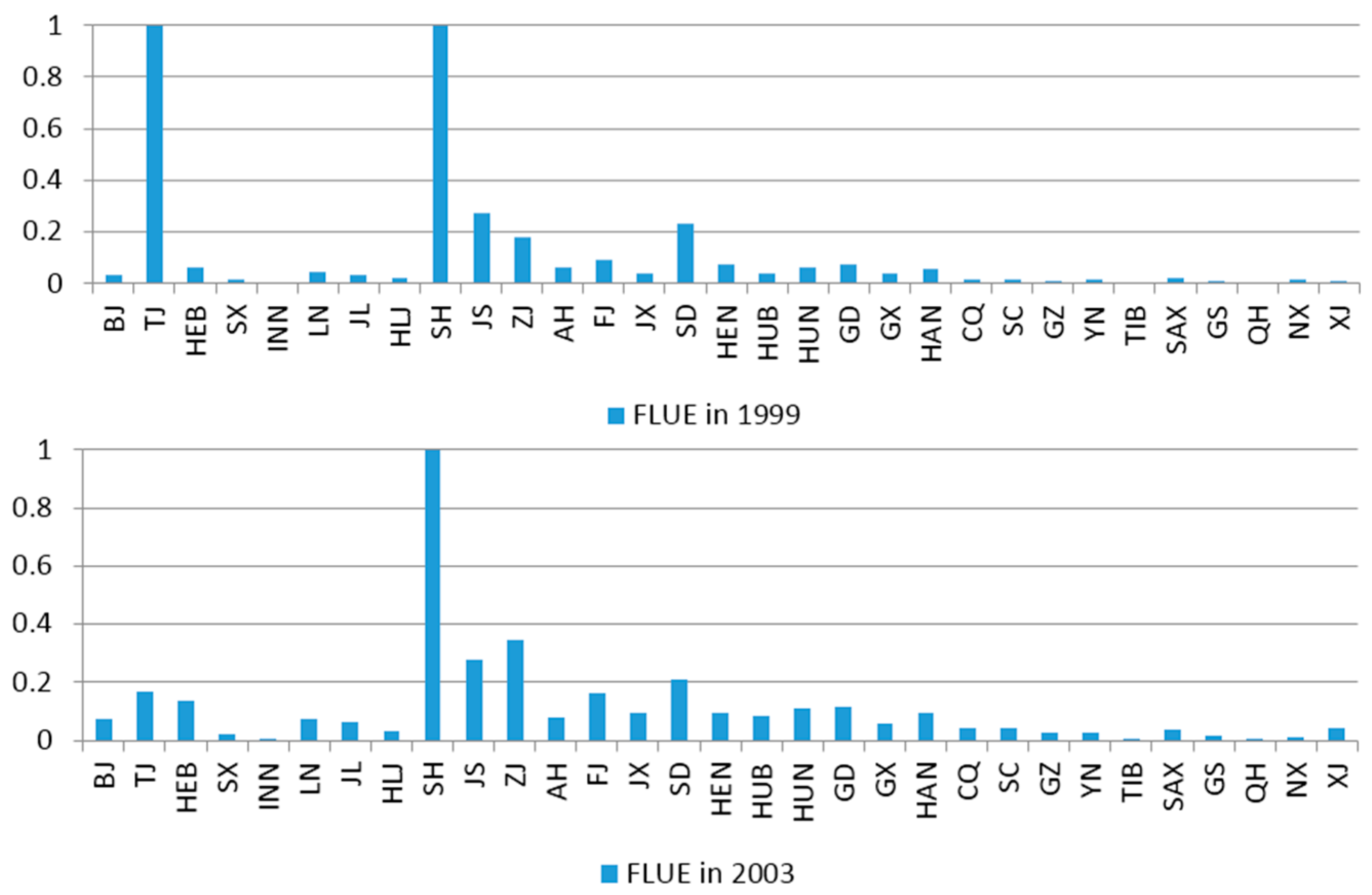
Figure 3 shows the FLUEs of the 31 provinces in representative years during the study period. In 1999, the FLUE values for Shanghai and Tianjin reached 1, which indicates that their forested land use was at the forefront of production technology. The remaining provinces were in an inefficient state, especially Tibet, Inner Mongolia and Qinghai, which had FLUE values near zero. In 2003, the overall efficiency in China improved slightly. Shanghai was still at the forefront of production technology, whereas the FLUEs of Tibet, Inner Mongolia, and Qinghai remained in an inefficient state. In 2007, the growth trend of FLUE in China continued, especially in Liaoning, Jilin, Heilongjiang, Jiangsu, Zhejiang, Anhui, Fujian, Jiangxi, Shandong, Henan, Hubei, Hunan, Guangdong, Guangxi, and Hainan. Shanghai still had the highest efficiency in forested land use, whereas the FLUEs of Tibet, Inner Mongolia, and Qinghai were still in an inefficient state. In 2010, there were obvious improvements in FLUE: the number of provinces with FLUE values equal to 1 increased to 6; the remaining provinces continued to increase their values, with the exception of Tibet, Inner Mongolia, and Qinghai. In summary, the FLUE of Shanghai was always highest, whereas Tibet, Inner Mongolia, and Qinghai suffered the most inefficiency in forested land use with efficiency values near zero, indicating that forested land use cannot produce enough economic output.
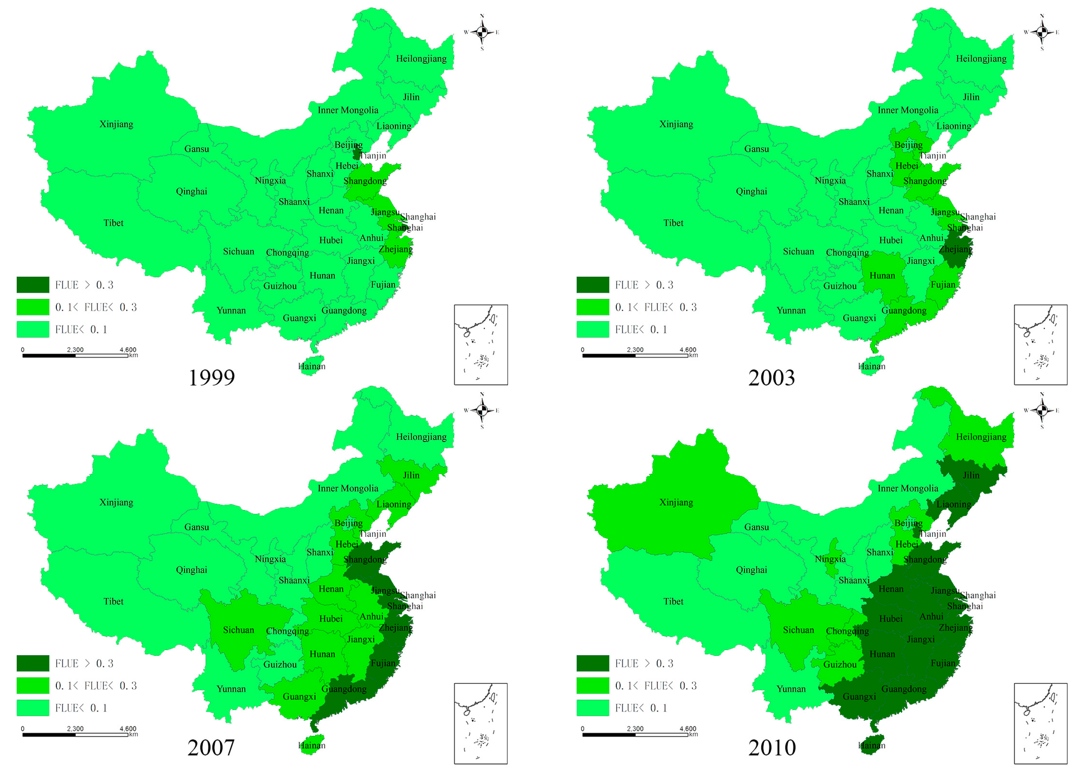
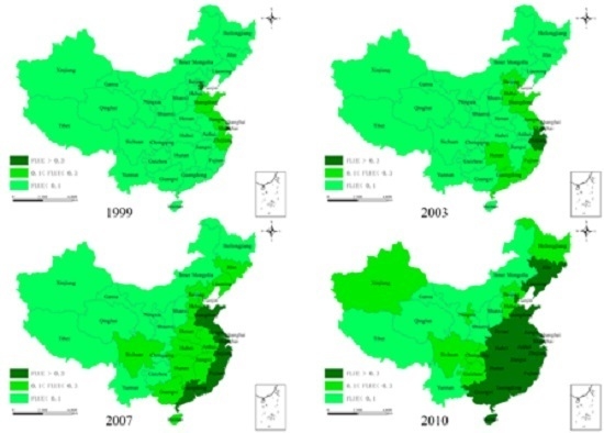
To discover the spatiotemporal difference in the FLUEs of the 31 provinces, we used the Natural Breaks tool in Arcgis10.2 software (ESRI, Redlands, CA, USA) to classify their FLUEs. The results are shown in Figure 4.
The spatiotemporal pattern change of forested land use efficiency (FLUE) in China is displayed in Figure 4. In 1999, there were two eastern coastal municipalities (Tianjin and Shanghai) with FLUE values greater than 0.3, three eastern coastal provinces (Shandong, Zhejiang, and Jiangsu) with FLUE value between 0.1 and 0.3 and the remaining provinces had FLUE values of less than 0.1. In 2003, the spatiotemporal pattern changed slightly, the FLUEs of Shanghai and Jiangsu were the highest and the number of provinces with FLUE values between 0.1 and 0.3 increased to 6. In 2007, the number of provinces with FLUE value greater than 0.1 increased to 18, the provinces with FLUE values greater than 0.3 were mainly distributed in southeastern coast China, the provinces with FLUE values between 0.1 and 0.3 contained the 6 provinces of Mid-China, two northeastern provinces, a province on the North China Plain, and a province in southwestern China. In 2010, the trend of growth in FLUE continued to extend to the west, which is highlighted by the expanded number of provinces with FLUE values greater than 0.3. On the whole, forested land use efficiency in China shows obvious regional differences, presenting a declining trend from east to west with the exception of several provinces.

4.2. Influential Factors in Regional FLUE Differences

It is easy to associate regional socioeconomic differentiation and regional climate differences with the obvious regional differences of FLUE. Hence, we selected potential explanatory variables based on a literature review of each category (demography, economy, societies and arctic climate) [39,40,41]. Three variables were selected to indicate demography: total population, population density, and nonagricultural population proportion. Gross domestic product, total forestry output, the proportion of secondary industry, the proportion of tertiary industry, and tourism revenue in forestry were selected for economy. Four variables were selected to indicate social activities: foreign investment in forestry, road mileage, railway mileage, and number of employees in forestry [41]. Two variables were selected to indicate arctic climate. A correlation analysis and principal component analysis were also applied to select the most important indicator. The final set included nine indicators: population density (PD), proportion of nonagricultural population (PNAP), gross domestic product per capita (PGDP), total forestry output (TFO), investment in fixed assets (IFA), road mileage (RM), land urbanization rate (LUR), annual rainfall (AR), and annual average temperature (AAT). Moreover, the Moran’s I index [42] was calculated to examine the autocorrelation of the variables. The results showed that the global Moran’s I values were not statistically significant, indicating that no spatial autocorrelation exists. There will be a very natural difference among different cross-sectional data and different individual values, so we built a fixed effects regression model based on panel data. The model is as follows:
l n   y i t = α i t + β 1 l n   I F A i t + β 2 l n   T F O i t + β 3 P G D P i t + β 4 l n   P D i t + β 5 A R i t + β 6 A A T I T                             + β 7 R M i t + β 8 P N A P + β 9 L U R i t + μ i t
where i and t (t = 1999, …, 2010) represent province i and year t, respectively. The term α i t is a constant, and μ i t is the random error term. The term y i t is the FLUE value for province i. The regression result is shown in Table 1.
The adjusted R-squared is 0.6768, which indicates that the results explain the model reasonably well. From the results of the p value, we know that the coefficients of the land urbanization rate (LUR) and the proportion of nonagricultural population (PNAP) are statistically significant. The positive coefficients imply that the land urbanization rate and proportion of nonagricultural population had a significant positive impact on FLUE in China. The land urbanization rate and the proportion of nonagricultural population measure urbanization from two different perspectives; the common results of the improvement of the two indicators are increasing demand in all types of products, and forestry products are no exception. Population density (PD) was also an important factor influencing forested land use efficiency; similar to LUR and PNAP, population density had an impact on the demand for forestry products. The coefficient of gross domestic product per capita (PGDP) is statistically significant at the 10% level, the positive coefficient indicates that economic development will promote the efficiency. We did not find specific evidence that climate factors have a significant impact on the spatial differentiation of forested land use efficiency in China from the results of this regression.

4.3. NMPFI and Its Decompositions

We know that there was an obvious spatial differentiation of forested land use efficiency in China. According to geographical closeness and forestry development, we divided the 31 provinces across China into three regions: eastern (E), central (C) and western (W). The eastern region includes three municipalities (Beijing, Tianjing, and Shanghai) and eight coastal provinces (Hebei, Liaoning, Jiangsu, Zhejiang, Fujian, Shandong, Guangdong, and Hainan). This region enjoys advanced production technology and well-developed transportation. The central region consists of eight inland provinces (Shanxi, Jilin, Heilongjiang, Anhui, Jiangxi, Henan, and Hunan); this region is famous for its high resource consumption. The western region consists of one municipality (Chongqing) and eleven inland provinces and autonomous regions (Inner Mongolia, Xinjiang, Gansu, Qinghai, Shaanxi, Ningxia, Sichuan, Yunnan, Guizhou, Guangxi, and Tibet). This region has poor economic development.
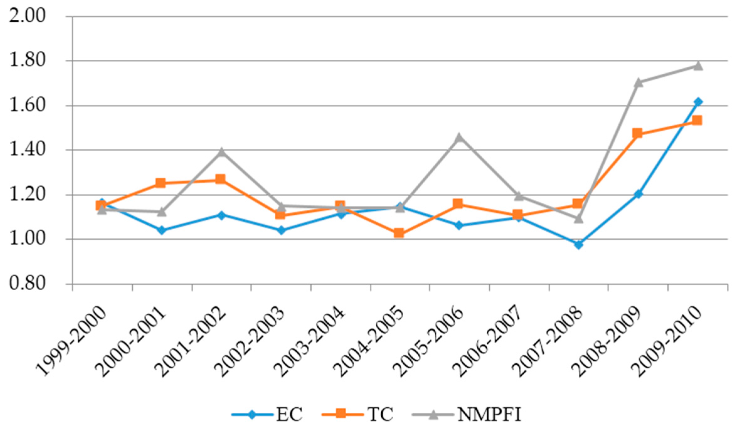
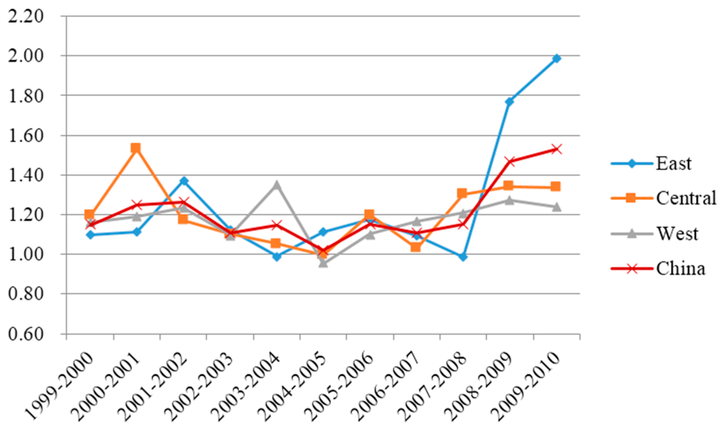
According to Equations (7) and (8), we computed the NMPFI and its decompositions of forested land productivity. Figure 5 shows the trends of the NMPFI and its decompositions in China during the study period. We find that the NMPFIs in China were always above 1, indicating that the productivity of forested land in China was always increasing. There were three peak values, corresponding to the period from 2001 to 2002, the period from 2005 to 2006, and the period from 2009 to 2010, and a valley value corresponding to the period from 2007 to 2008. The NMPFI grew rapidly after the year 2008, which was consistent with the time of introduction the policy of “opinions on comprehensively promoting the reform of collective forest right system” [38]. During the period of 1999–2007, the trend for EC was relatively stable, and the values were always above 1, indicating that the efficiency change was progressing. During the 2007–2008 period, the EC was less than 1, indicating that the efficiency change suffered deterioration. After 2008, the EC rocketed, and the value of EC reached 1.60 during the period from 2009 to 2010. The trend for TC was always above 1, indicating that technological change was progressing during the study period. We find that the change in forested land productivity in the whole country was the interactive effect of these two decompositions.
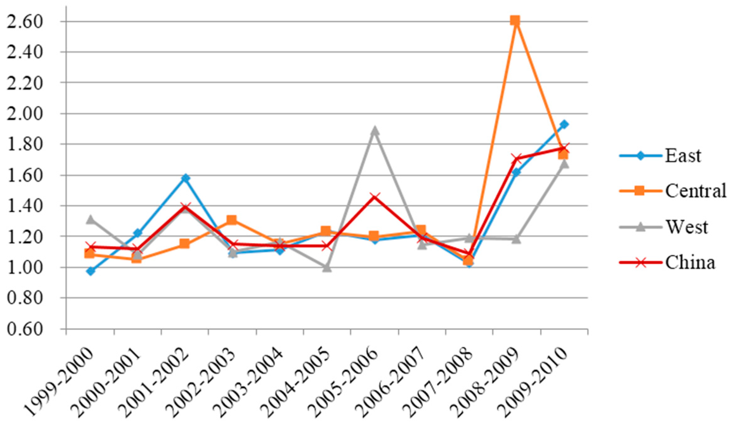
With regard to the NMPFI and its decompositions in the three regions, Figure 6, Figure 7 and Figure 8 show the changing trends of the NMPFI, EC, and TC, respectively.
From Figure 6, we know that the trend in the NMPFI in the eastern region was similar to the trend in China, except for the period from 1999 to 2000. During the 1999–2000 period, the NMPFI of the eastern region was less than 1, indicating that its forested land productivity had suffered deterioration. Combining the results of Figure 7 and Figure 8 indicates that the changes in the productivity of the forested land in the eastern region derived mostly from the progress of technology change. The NMPFIs in the central region were always above 1. During the period from 2008 to 2009, the NMPFI reached 2.6, and the progress of forested land productivity in the central region derived mostly from the progress of the efficiency change shown in Figure 7 and Figure 8, which was different from the eastern region. The trend of the NMPFI in the western region shows larger fluctuations. Its valley value appeared in the period from 2004 to 2005, and the NMPFI was less than 1, indicating that the forested land productivity suffered deterioration. The peak value appeared in the 2005–2006 period. Combining the results of Figure 6 and Figure 7 indicates that the change in the productivity of the forested land in the western region was the interactive effect of these two decompositions.

4.4. Convergences

From the previous analysis, we know that there were large differences in the evolving trends among the three regions. Will the difference between the regions be reduced over time? Do the regions show the same convergence pattern? The concept of convergence originates from neoclassical economics, which applies this tool to analyze differences in per capita income among regions [43]. Here, we used the method to analyze the disparity of the NMPFIs among the three regions. The convergence usually contains σ-convergence and β-convergence, and β-convergence also includes two types of convergence called absolute convergence and conditional convergence. The σ-convergence exists if there is a clear decline in the standard deviation over time, which indicates that the NMPFI gap among regions has gradually been narrowing. Absolute β-convergence exists if the coefficient of β is significantly negative, which implies that the efficiencies for all provinces in a certain region converge to the same steady state. In addition, conditional β-convergence exists if the coefficient of β is significantly negative, which implies that the efficiencies of provinces in different regions converge to their own steady state [44]. Their formulas are as follows:
  • σ-convergence:
    σ t = [ i = 1 n ( ln Y i , t 1 n i = 1 n ln Y i , t ) 2 ] n
  • absolute β-convergence:
    1 T ln ( Y i , t + T Y i , t ) = α 0 + β 0 ln Y i , t + ε i , t
  • conditional β-convergence:
    1 T ln ( Y i , t + 1 Y i , t ) = α 1 + β 1 ln Y i , t + j = 1 J γ j x i , t j + ε i , t
where α 0 and α 1 are constants and i = 1, …, n represents the provinces. Y represents the NMPFI, and x i , t j is the jth influencing factors of the ith province in period t. T is the study period, and ε i , t is the stochastic error.

4.4.1. σ-Convergence

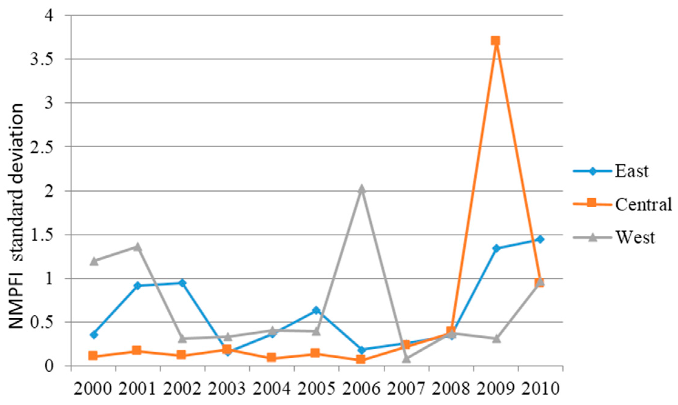
The result of σ-convergence is shown in Figure 9. We find that σ-convergence did not exist in the three regions because the NMPFI gaps in all the regions have fluctuated continuously in the figure, indicating that the gaps did not narrow in the study period. The standard deviation of the NMPFI in the western region ranked first with 0.70, and the central region ranked last with 0.55. These results indicate that the NMPFI gap among provinces in the western region was greater than the gap in other regions.

4.4.2. Absolute β-Convergence

According to Equation (11), we obtained the result of absolute β-convergence as shown in Table 2. The β-convergence model fits well in the western region, where its coefficient β is significantly negative, indicating that absolute β-convergence existed in the western region: the NMPFI values of all the provinces in the western region converged to the same steady state. The coefficient β of the eastern region is also significantly negative, but the adjusted R-squared is not high, therefore, the model cannot fit well. Because the coefficient β of the central region is not statistically significant and the adjusted R-squared is very low, absolute β-convergence did not exist in the region; that is to say, the NMPFI of all of the provinces in the central region did not converge to the same steady state.

4.4.3. Conditional β-Convergence

According to Equation (12), we obtained the result of conditional β-convergence, shown in Table 3. We find that the values of coefficient β in the three regions are all significantly negative, whereas the adjusted R-squared values are not high; thus so that they cannot explain the actual situation well.

5. Discussion and Conclusions

5.1. Conclusions

This paper used the GGDDF model to measure the forested land use efficiency in China and 31 provinces during the period from 1999 to 2010. In this country, forested land use efficiency continued to increase during the study period. The FLUE of Shanghai was always highest, whereas Tibet, Inner Mongolia, and Qinghai suffered the most inefficiency in forested land use. From the spatial perspective, a declining trend was observed from east to west, with the exception of several provinces. There were obvious spatial differences in forested land use efficiency among the 31 provinces. According to the fixed effects regression model based on panel data—which considers population density (PD), proportion of non-agricultural population (PNAP), gross domestic product per capita (PGDP), total forestry output (TFO), investment in fixed assets (IFA), road mileage (RM), land urbanization rate (LUR), annual rainfall (AR), and annual average temperature (AAT) as independent variables—urbanization, the economic development situation, and population density were the main influencing factors in spatial differences in forested land use efficiency.
Because of the obvious spatial differences in the forested land use efficiency among the provinces, we divided them into three regions (eastern region, central region, and western region). Then, by using the GML model, we analyzed forested land performance and its decompositions for China and the three regions. For the eastern region, the NMPFIs were always above 1 after 2000, indicating that the productivity of forested land was always increasing, and the change in the productivity of forested land in the eastern region derived mostly from the progress of technological change. For the central region, the NMPFIs were always above 1, and the progress in forested land productivity derived mostly from the progress of efficiency change. For the western region, the trend in the NMPFI had larger fluctuations, and the change in the productivity of forested land in the western region was the interactive effect of these two decompositions. Finally, the results of convergence tell us that only in the western region did an absolute β-convergence exist; that is to say, the NMPFI of all the provinces in the western region converged to the same steady state.

5.2. Discussion

In this study, we attempted to calculate the efficiency of a specific input (forested land) and to explore the mechanisms that influence spatiotemporal changes to this input. However, there are still some limitations. First, we adopted only an 11-year sample period because of the unavailability of data. We will try to obtain more data to extend the study period to produce more convincing and meaningful results. Second, some factors that play important roles in determining the forested land use efficiency were not considered in this paper for the same reason. Third, economic externalities are not considered in the econometric model, although forested land not only provides economic outputs but also ecosystem services. However, economic efficiency was the main research object in this paper; therefore, we ignored the ecological efficiency. Last, although this paper attempted to explore forested land use efficiency and its spatiotemporal patterns, uncertainty may still exist; thus, methods for verifying our evaluation will be considered in future work. We will make improvements to these limitations in future studies.

Acknowledgments

This study was supported by the National Natural Science Foundation of China, No. 41561040; the Key projects of the National Social Science Fund of China, No. 15AZD075; the Key projects of the social science fund of Jiangxi Province in China, No. 15ZQZD10; the Natural Science Foundation of Jiangxi Province No. 20143ACB21023; the Technology Foundation of Jiangxi Education Department of China, No. KJLD14033; the Fok Ying-Tung Fund, No. 141084.

Author Contributions

Yafen He and Hualin Xie had the original idea for the study. Yafen He was responsible for data collecting. Yafen He, Yuanhua Fan, Wei Wang, Xue Xie and Hualin Xie carried out the analyses. All the authors drafted the manuscript, and approved the final one.

Conflicts of Interest

The authors declare no conflict of interest.

References

  1. State Forest Administration (SFA). The National Forest Resources Statistics—The Seventh National Forest Resources Inventory; State Forest Adminstration: Beijing, China.
  2. Su, S.; Wang, Y.; Luo, F.; Mai, G.; Pu, J. Peri-urban vegetated landscape pattern changes in relation to socioeconomic development. Ecol. Indic. 2014, 46, 477–486. [Google Scholar] [CrossRef]
  3. Xie, X.; Xie, H.; Fan, Y. Spatiotemporal Patterns and Drivers of Forest Change from 1985–2000 in the Beijing–Tianjin–Hebei Region of China. J. Resour. Ecol. 2016, 7, 301–308. [Google Scholar] [CrossRef]
  4. Hoek, J.; Ozdogan, M.; Burnicki, A.; Zhu, A. Evaluating forest policy implementation effectiveness with a cross-scale remote sensing analysis in a priority conservation area of Southwest China. Appl. Geogr. 2014, 47, 177–189. [Google Scholar] [CrossRef]
  5. Sharma, S.; Pandey, D.; Agrawal, M. Global warning potential and sustainable management of three land uses in Varanasi. Manag. Environ. Qual. 2016, 27, 364–373. [Google Scholar] [CrossRef]
  6. Li, M.; Mao, L.; Zhou, C.; Vogelmann, J.; Zhu, Z. Comparing forest fragmentation and its drivers in China and the USA with Globcover v2.2. J. Environ. Manag. 2010, 91, 2572–2580. [Google Scholar] [CrossRef] [PubMed]
  7. LeBel, G.; Stuart, W.B. Technical Efficiency Evaluation of Logging Contractors Using a Nonparametric Model. Int. J. For. Eng. 1998, 9, 15–24. [Google Scholar]
  8. Viitala, E.J.; Hänninen, H. Measuring the Efficiency of Public Forestry Organizations. For. Sci. 1998, 44, 298–307. [Google Scholar]
  9. Lee, J.Y. Using DEA to measure efficiency in forest and paper companies. For. Prod. Soc. 2005, 55, 58–66. [Google Scholar]
  10. Salehirad, N.; Sowlati, T. Productivity and efficiency assessment of the wood industry: A review with a focus on Canada. For. Prod. Soc. 2006, 56, 25–32. [Google Scholar]
  11. Lai, Z.; Zhang, Z. The DEA analysis of Guangdong forestry input-output efficiency. Issues For. Econ. 2008, 28, 323–326. (In Chinese) [Google Scholar]
  12. Lai, Z.; Zhang, Z. The super-efficiency DEA analysis of Guangdong forestry input-output. J. South China Agric. Univ. 2008, 7, 43–48. (In Chinese) [Google Scholar]
  13. Shi, L.; Zhang, C. Management efficiency analysis of farmer’s forest land based on the DEA method. Issues For. Econ. 2012, 32, 235–326. (In Chinese) [Google Scholar]
  14. Li, C.; Li, N.; Luo, H.; Wang, B. The efficiency analysis and path optimization of forestry input-output in China based on data envelopment analysis. Chin. Agric. Sci. Bull. 2011, 27, 55–59. (In Chinese) [Google Scholar]
  15. Tian, S.; Xu, W. Evaluation of China’s forestry input-output efficiency based on DEA modeling. Resour. Sci. 2012, 34, 1944–1950. (In Chinese) [Google Scholar]
  16. Lambin, E.F.; Baulies, X.; Bockstael, N. Land-Use and Land-Cover Change (LUCC): Implementation Strategy; A Core Project of the International Geospere-Biosphere Programme and the International Human Dimensions Programme on Global Environmental Change; IGBP Report 48, IHdp. Report 10; IGBP: Stockbolm, Sweden, 1995; p. 125. [Google Scholar]
  17. Ojima, D.; Lavorel, S.; Graumlich, L. Terrestrial Human-Environment Systems: The Future of Land Research in IGBP II. IGBP Glob. Chang. Newslett. 2005, 50, 31–34. [Google Scholar]
  18. Turner, B.L.; Skole, D.; Sanderson, S. Land Cover Change Science/Research Plan; IGBP Report No.35, HDP Report 7; IGBP of the ICSU: Stockholm, Sweden; HDP of the ISSC: Geneva, Switzerland, 1995. [Google Scholar]
  19. IGBP Secretariat. GLP Science Plan and Implementation Strategy; IGBP Report No. 53, IHDP Report No. 19; IGBP: Stockholm, Sweden, 2005; p. 64. [Google Scholar]
  20. Turner, B.L., II; Lambin, E.F.; Reenberg, A. The emergence of land change science for environmental change and sustainability. Proc. Natl. Acad. Sci. USA 2007, 104, 20666–20671. [Google Scholar]
  21. Xie, H.; Wang, W. Spatiotemporal differences and convergence of urban industrial land use efficiency for China’s major economic zones. J. Geogr. Sci. 2015, 25, 1183–1198. [Google Scholar] [CrossRef]
  22. Wang, W.; Xie, H.; Jiang, T.; Zhang, D.; Xie, X. Measuring the Total-Factor Carbon Emission Performance of Industrial Land Use in China Based on the Global Directional Distance Function and Non-Radial Luenberger Productivity Index. Sustainability 2016, 8, 336. [Google Scholar] [CrossRef]
  23. Tone, K. A slacks-based measure of efficiency in data envelopment analysis. Eur. J. Oper. Res. 2001, 130, 498–509. [Google Scholar] [CrossRef]
  24. Yang, L.; Wu, W.; Su, Q.; Jiang, X.; Wei, Y. Evaluation of road transport efficiency in China during 1997–2010 based on SBM-Undesirable model. Prog. Geogr. 2013, 32, 1602–1611. [Google Scholar]
  25. Pan, D.; Ying, R. Agricultural eco-efficiency evaluation in China based on SBM model. Acta Ecol. Sin. 2013, 33, 3837–3845. [Google Scholar] [CrossRef]
  26. Yang, Q.; Duan, X.; Ye, L.; Zhang, W. Efficiency evaluation of city land utilization in the Yangtze River Delta using a SBM-Undesirable model. Resour. Sci. 2014, 36, 712–721. [Google Scholar]
  27. Zhang, Y.; Jin, P.; Feng, D. Does civil environmental protection force the growth of China’s industrial green productivity? Evid. Perspect. Rent-Seek. 2015, 51, 215–227. [Google Scholar]
  28. Xie, H.; Wang, W.; Yang, Z.; Choi, Y. Measuring the sustainable performance of industrial land utilization in major industrial zones of China. Technol. Forecast. Soc. Chang. 2016. [Google Scholar] [CrossRef]
  29. Zhang, N.; Choi, Y. Total-factor carbon emission performance of fossil fuel power plants in China: A meta frontier non-radial Malmquist index analysis. Energy Econ. 2013, 40, 549–559. [Google Scholar] [CrossRef]
  30. Colinoa, A.; Benito-Osoriob, D.; Rueda-Armengotc, C. Entrepreneurship culture, total factor productivity growth and technical progress: Patterns of convergence towards the technological frontier. Technol. Forecast. Soc. Chang. 2014, 88, 349–359. [Google Scholar] [CrossRef]
  31. Xiong, Q.; Guo, G. Study on the efficiency difference of city industrial land production across provinces in China. Resour. Sci. 2013, 35, 910–917. (In Chinese) [Google Scholar]
  32. Wang, Z.; Feng, C. A performance evaluation of the energy, environmental, and economic efficiency and productivity in China: An application of global data envelopment analysis. Appl. Energy 2015, 147, 617–626. [Google Scholar] [CrossRef]
  33. Zhang, N.; Kong, F.; Choi, Y. Measuring sustainability performance for China: A sequential generalized directional distance function approach. Econ. Model. 2014, 41, 392–397. [Google Scholar] [CrossRef]
  34. Zhang, N.; Choi, Y. A note on the history on the evolution of directional distance function and its development in energy and environmental studies 1997–2013. Renew. Sustain. Energy Rev. 2014, 33, 50–59. [Google Scholar] [CrossRef]
  35. Oh, D. A global Malmquist-Luenberger productivity index. J. Product. Anal. 2010, 34, 184–197. [Google Scholar] [CrossRef]
  36. National Bureau of Statistics of China (NBSC). China Forestry Statistical Yearbook. Available online: http://www.stats.gov.cn/tjsj/ndsj/ (accessed on 23 May 2012). (In Chinese)
  37. Kong, F.; Wu, X.; Liao, W. Factors decomposition and calculation of contribution ratio of forestry science and technology advancement in 31 provinces (cities, autonomous regions) from 2002–2011. J. Agro-For. Econ. Manag. 2014, 13, 420–428. (In Chinese) [Google Scholar]
  38. The Central People’s Government of the People’s Republic of China (CPGPRC). Available online: http://www.gov.cn/jrzg/2008-07/14/content_1044403.htm (accessed on 14 June 2008).
  39. Su, S.; Zhou, X.; Wan, C.; Li, Y.; Kong, W. Land use changes to cash crop plantations: crop types, multilevel determinants and policy implications. Land Use Policy 2016, 50, 379–389. [Google Scholar] [CrossRef]
  40. Liu, Y.; Feng, Y.; Zhao, Z.; Zhang, Q.; Su, S. Socioeconomic drivers of forest loss and fragmentation: A comparison between different land use planning schemes and policy implications. Land Use Policy 2016, 54, 58–68. [Google Scholar] [CrossRef]
  41. Deng, X.; Huang, J.; Uchida, E.; Rozelle, S.; Gibson, J. Pressure cookers or pressure valves: Do roads lead to deforestation in China? J. Environ. Econ. Manag. 2011, 61, 79–94. [Google Scholar] [CrossRef]
  42. Moran, P. The interpretation of statistical maps. J. R. Stat. Soc. Ser. B 1948, 10, 243–251. [Google Scholar]
  43. Solow, R. A contribution to the theory of economic growth. Q. J. Econ. 1956, 70, 65–94. [Google Scholar] [CrossRef]
  44. Sala-i-Martin, X. Regional cohesion: Evidence and theories of regional growth and convergence. Eur. Econ. Rev. 1996, 40, 1325–1352. [Google Scholar] [CrossRef]
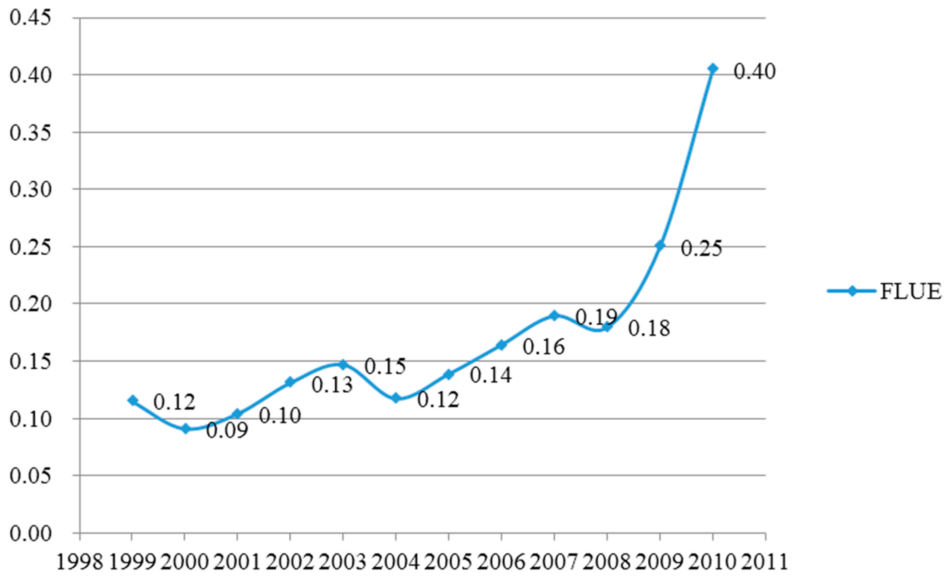
Figure 1. Forested land use efficiency in China from 1999 to 2010.
Sustainability 08 00772 g001
Figure 2. Variation of input factors from 1999 to 2010.
Sustainability 08 00772 g002
Figure 3. The forested land use efficiency (FLUE) of 31 provinces in China from 1999 to 2010. Abbreviation: Beijing (BJ), Tianjin (TJ), Hebei (HEB), Shanxi (SX), Inner Mongolia (INN), Liaoning (LN), Jilin (JL), Heilongjiang (HLJ), Shanghai (SH), Jiangsu (JS), Zhejiang (ZJ), Anhui (AH), Fujian (FJ), Jiangxi (JX), Shandong (SD), Henan (HN), Hubei (HUB), Hunan (HUN), Guangdong (GD), Guangxi (GX), Hainan (HAN), Chongqing (CQ), Sichuan (SC), Guizhou (GZ), Yunnan (YN), Tibet (TIB), Shannxi (SAX), Gansu (GS), Qinghai (QH), Ningxia (NX), Xinjiang (XJ).
Sustainability 08 00772 g003aSustainability 08 00772 g003b
Figure 4. Spatiotemporal pattern change of forested land use efficiency (FLUE) in China.
Sustainability 08 00772 g004
Figure 5. Trends of the non-radial Malmquist forested land performance index (NMFLPI) and its decompositions in China.
Sustainability 08 00772 g005
Figure 6. Trends in the NMFLPI for different regions.
Sustainability 08 00772 g006
Figure 7. Trends in efficiency change (EC) for different regions.
Sustainability 08 00772 g007
Figure 8. Trends in technological change (TC) for different regions.
Sustainability 08 00772 g008
Figure 9. Trends in the NMFLPI standard deviation in regions.
Sustainability 08 00772 g009
Table 1. Result of regression. *** p < 0.001, ** p < 0.05, * p < 0.01.
Coefficientp Value
Ln IFA−0.04198410.399
Ln TFO0.03383530.477
PGDP0.00214110.092 *
Ln PD0.35252660.041 **
AR0.3688720.141
AAT0.02356760.251
RM−0.610590.426
PNAP0.0244450.014 **
LUR0.03030610.000 ***
adjusted R-squared = 0.6768
Table 2. Absolute β-convergence results for the NMPFI. ** p < 0.05, * p < 0.01.
Eastern RegionCentral RegionWestern Region
constant0.046 *0.043 *0.039 *
(2.862)(2.492)(3.434)
ln Y i , 0 −0.078 *−0.096−0.113 **
(−2.72)(−0.679)(−4.869)
Adjusted R-squared0.4510.0710.703
Table 3. Conditional β-convergence results for the NMPFI. *** p < 0.001, * p < 0.01.
Eastern RegionCentral RegionWestern Region
constant0.016 *0.021 ***0.017 *
(3.791)(4.610)(2.391)
ln Y i , 0 −0.109 ***−0.108 ***−0.091 ***
(−12.603)(−10.060)(−10.870)
Adjusted R-squared0.5950.5640.500