Conjoint Analysis of Farmers’ Response to Conservation Incentives

Abstract

Environmental degradation threatens the long term resiliency of the US food and farming system. While USDA has provided conservation incentives for the adoption of best management practices (BMPs), only a small percentage of farms have participated in such conservation programs. This study uses conjoint analysis to examine Vermont farmers’ underlying preferences and willingness-to-accept (WTA) incentives for three common BMPs. Based on the results of this survey, we hypothesize that federal cost share programs’ payments are below preferred incentive levels and that less familiar and more complex BMPs require a higher payment. Our implications focus on strategies to test these hypotheses and align incentive payments and other non-monetary options to increase BMP adoption.

1. Introduction

The environmental degradation and negative externalities imposed on society by US agricultural production systems have been steadily increasing since the end of World War II [1]. These impacts include soil erosion, pollution of waterways and groundwater, greenhouse gas emissions, loss of biodiversity, shrinking wildlife habitat, pesticide and fertilizer run-off, and leaching [2]. Current trends in population growth and demand for food continue to fuel the production of these externalities [1]. Climate change and variability will further compound the effects of these challenges to the long-term sustainability of agricultural systems [3]. The need to ensure the resiliency and viability of our farms and food systems is a pressing and increasingly salient issue.

The USDA and other agricultural technical service providers have emphasized the need for farmers to adopt best management practices (BMPs) to address environmental health concerns, ensure the long-term sustainability of their operations, and to use as an adaptation strategy for coping with climate change [3]. BMPs are defined by the USDA as “established soil conservation practices that also provide water quality benefits” [4]. Federal conservation programs offer incentive payments which cost-share the implementation of BMPs with farmers. However, in 2012, only 2.2% of agricultural acreage in the United States had an active or completed contract through the Environmental Quality Incentives Program (EQIP) [5,6]. This raises many questions, including whether the incentive levels offered by this federal programs match farmers’ financial requirements to implement BMPs. This study uses conjoint analysis to determine Vermont farmers’ underlying preferences and willingness-to-accept (WTA) incentive levels for three common BMPs. The results complement a parallel study in which BMP implementation costs were directly measured on farms [7]. Results highlight regional farmer decision-making and preferences for conservation practices while further informing the design of voluntary conservation programs that assist farmers in improving the health of their land and the resiliency of their operations [8,9,10].

Incentivizing BMP Adoption

Several factors, both economic and non-economic, influence farmers’ decision to adopt BMPs. BMPs are more likely to be adopted by farmers whose peer networks support and promote the practices [11]. Innovations which mesh well with farmers’ perceptions of self, socioeconomic status, and background and which preserve their primary source of social capital have a greater likelihood of being adopted [11,12]. In addition, farmers with diversified operations and those who derive intangible value from the health of their land are more likely to implement BMPs [13,14,15]. This is significant because sustainable agricultural practitioners by nature tend to be reflexive, rather than prescriptive, growers, a valuable quality given the unpredictability of the farming profession [16]. Farm scale is positively correlated to adoption, with larger farms more likely to adopt BMPs [13,14,17]. The BMPs which are most frequently adopted are generally low in complexity, highly compatible with the existing farm system, high in trialability, and high in observability [18].

Economics governs farmers’ decisions to adopt BMPs, perhaps more than any other factor [15,19]. The practice needs to be profitable and the perceived threats of harm high enough in order for widespread adoption to occur [18,20,21,22]. An adopted practice is considered profitable when the benefits produced outweigh both the direct costs and opportunity costs of implementation [23,24]. However, analysis of BMP profitability is not always straightforward; the private benefits of implementation may only be tangible in the medium or long term while costs are accrued in the short term [12,24,25]. In addition, implementation of BMPs may create positive externalities in the form of ecosystem services; if the costs of implementation are greater than the private benefits produced, farmers are privately funding public goods [26,27]. As public goods are non-rival and non-excludable, if farmers do not perceive enough potential harm to their farm systems to warrant adoption, they will be better off financially not implementing a BMP regardless of any existing environmental concerns; this lack of proactive adoption can result in the underproduction of ecosystem services and is detrimental to both the farm operation and society [26,27,28].

Federal conservation programs are one way to overcome farmers’ economic barriers to their adoption of conservation practices, incentivize production of public goods, and encourage the prosperity of agricultural systems without sacrificing environmental health [27,29]. These programs incentivize the supply of conservation practices by cost-sharing up to 75% of the implementation expenses. Payments are designed to partially compensate farmers for the direct costs incurred and provide a risk premium to offset the uncertainty associated with adoption [30,31]. However, it is challenging to set incentive levels that are cost-effective for both farmers and the federal government and that also address well-known principal-agent problems associated with moral hazards and bureaucratic over- or under-supply. Determining accurate figures for farmers’ willingness-to-accept (WTA) for implementing conservation practices that generate ecosystem services is a key step in designing efficient public policy and one that needs a continued regional research focus [30,32,33]. This study contributes to that aim.

In a parallel study, Helling et al. [7] measured costs of implementation (of three BMPs (cover cropping, management intensive rotational grazing (MIRG), and riparian buffer strips) on a set of 11 diversified Vermont farms. The average annual cost of implementation on these farms was $129.24/acre for cover cropping, $79.82/acre for MIRG, and $807.33/acre for riparian buffer strips.

Numerous studies over the years have used a variety of methods to measure farmer WTA to adopt BMPs. Bateman et al. [34] used 19 face to face interviews to elicit WTA to convert land to public woodlands (roughly analogous to riparian buffers); they found farmers required a risk premium reflecting income greater than expected revenue from farming. The mean WTA value was 121 pounds/acre (about $312 in current dollars). They describe the results as robust despite a small sample size. Cooper and Keim [35] used field level surveys of approximately 1000 farms in four US watersheds, asking farmers to accept or decline one of six payment values framing what the researchers believed would be likely WTA values for a set of water quality BMPs. The results suggest higher payments would encourage adoption by nonusers. Payments ranging from about $30–$70/acre resulted in 50% adoption by farmers. Zhong and Wu [36] used Contingent Valuation (CV) surveys of Kentucky farmers to calculate what percentage of implementation costs they would accept to implement water quality improvement practices. They find that, for conservation tillage and riparian buffers, perception of BMPs was more important than compensation for predicting adoption. Swinton and Harris [37] propose the use of procurement auctions to identify cost-effective incentives for water quality BMPs. Kim et al. [38] used also CV surveys to measure beef farmers’ willingness to adopt rotational grazing; higher payments increased probability of adoption and payments of about $90/acre encouraged 50 percent adoption. Ma et al. [39] used a Double Hurdle model to analyze survey data from 1700 Michigan farmers. Mean WTA for a suite of BMPs ranged from $10 to $50 per acre. Kingsbury and Boggess’ [40] logit analysis of Oregon farmer survey data found mean WTA figures of between $144 and $205 per acre (depending on farm type and location) to enroll in a conservation program including riparian strips.

There are at least three factors which may help determine the right price for a given good or service: (i) the break-even price (in this case, the cost of implementation) as a floor or lower bound; (ii) the reservation or WTA price, the price which will draw suppliers into the market; (iii) the going rate or market price (in this case, the current government payment). The Helling et al. [7] study provides the break-even price, while figures for the going rate are publicly available [5] and will be discussed below. The objective of this study is to measure the WTA price. Using a variety of complementary methods allows for comparison and triangulation. Our study complements the Helling et al. study in at least two ways. First, our study provides a stated choice perspective to the more revealed choice approach of Helling et al. Second, while the Helling et al. paper takes an idiographic approach (detailed cost information about eleven cases), our study uses a survey administered to a much larger and broader sample within a nomothetic approach. Our approach also analyzes how farmers weigh the relative costs and benefits of adopting three BMPs singly and in various combinations.

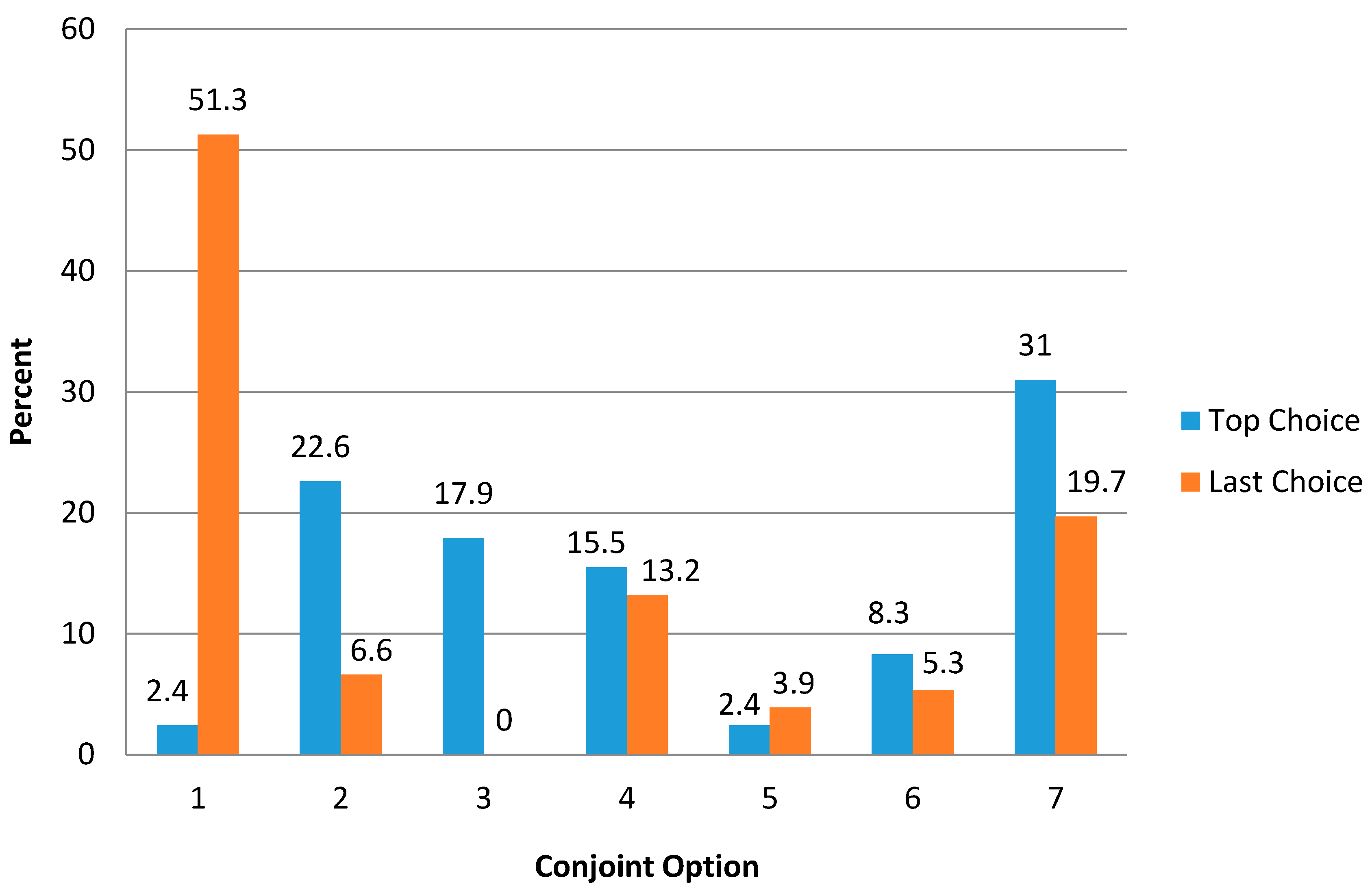
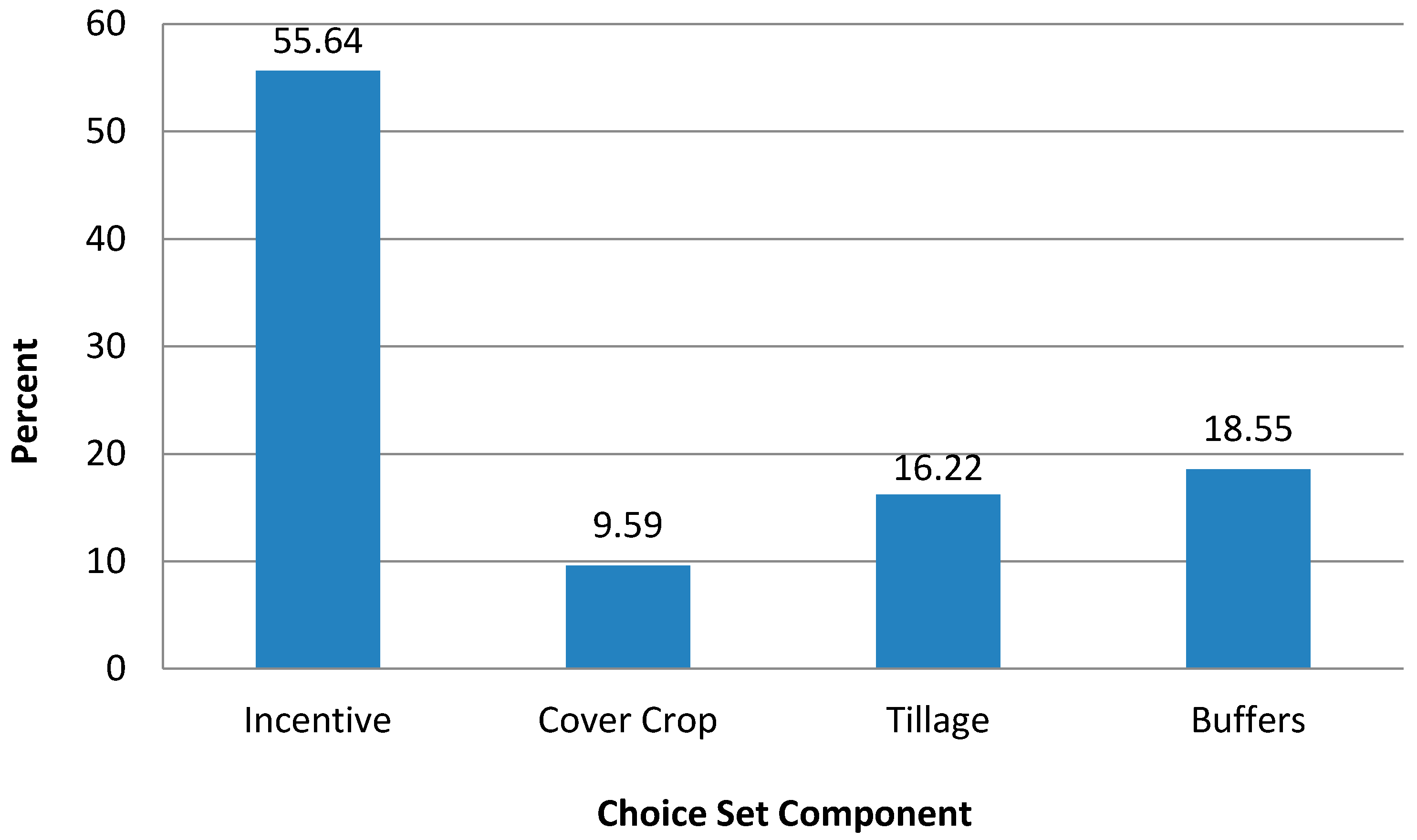
Specifically, in this study, conjoint analysis is used to examine the preferences and WTA incentive levels of Vermont farmers for implementing conservation tillage, cover cropping, and conservation buffer strips. We then compare the revealed WTA incentive levels of the farmers to studies using other methods and to the average offers made by the relevant federal program. Results will be used to develop hypotheses about WTA for BMPs implemented both singly and in combination.

2. Materials and Methods

2.1. Data Collection

Data for this project were collected using two different survey instruments. The target population of the initial survey was all farmers grossing over $10,000 in the Lamoille and Missiquoi watersheds in Vermont. The Lamoille watershed was selected because the land use distribution there is representative of the land use distribution in Vermont [41].The Missiquoi watershed was included to expand the coverage area and enable the aggregation of survey results with previous studies. The survey was designed by a transdisciplinary research team and data collected included farm characteristics, farmer demographics, on-farm presence of best management practices, use of conservation programs, and farmer perceptions of climate change [42]. The USDA National Agricultural Statistics Service (NASS) conducted the survey, identifying farmers in each watershed using zip codes. Due to the imperfect alignment of zip codes and ecological boundaries, some of the sampled farms may not lie within the watersheds; responses from these farmers were included in the study as it was decided their location was proximal enough to do so.

A screening postcard was mailed to all farmers with annual revenues greater than $1000 in the Lamoille and Missiquoi watersheds (N = 1104) in order to determine willingness to participate in the survey. A total of 220 screening postcards were returned, a response rate of 20%, with 114 farmers agreeing to take the full survey. The surveys were mailed in late March 2013 to those farmers as well as postcard respondents who had replied with a maybe or left that question blank. In total, 128 surveys were mailed. A follow-up phone call was placed three weeks later in an attempt to increase the response rate. In late June, phone surveys were conducted with farmers who had not yet responded on paper. The total number of completed surveys received was 79, a response rate of 62% for the subpopulation of postcard respondents but only a 6.5% response rate for the farmer population in the two watersheds.

Due to the fewer than anticipated responses, additional data were collected the following winter. The target population of that survey was Vermont farmers grossing over $1000; participants were recruited using convenience sampling. The instrument included structured and open-ended short answer questions designed to collect demographic data as well as information about conservation practices and conservation programs. Surveys were conducted in-person at an agricultural conference (N = 11), at a farmer interest group meeting (N = 6) and on-line (N = 44) generating a total of 61 completed surveys. The survey link was distributed through technical service providers’ agricultural listservs and newsletters as well as through a Vermont Agency of Agriculture listserv. An incentive was offered in exchange for participation. The distribution channels selected and utilized ensured that primarily farmers, rather than homesteaders or gardeners considered to have a farm under the census definition, completed this survey.

2.2. Demographic Analysis

Results from both surveys were combined and the demographic characteristics compared to ensure that no farmer had taken both surveys. All data analysis was performed using SPSS and included frequencies, descriptive statistics, Chi² crosstabs, and Independent Sample T-tests. Demographic differences between the following eight different respondent groupings were tested for significance: those who responded by mail compared to those who responded by phone to the first survey, respondents to the first survey compared to the second, and those who responded to the conjoint question compared to those who did not for all respondents combined and for respondents grouped by survey. In all of the analyses, the decision was made to classify all certified organic farmers and those who farm organically but are not certified together under organic, as those two groups tend to employ similar agricultural practices.

2.3. Conjoint Question Design

This study utilizes conjoint analysis to determine the preferences and WTA incentive levels of Vermont farmers for three different BMPs. A full profile rank order response mode with a part-worth conjoint model was used. The three BMPs selected for this study were cover cropping, conservation tillage, and conservation buffer strips.

Table 1. Combinations of conservation practices offered in conjoint question.

Option	Offered Price	Practices
1	30	Conservation tillage
2	90 *	Cover cropping
3	105	Conservation buffer strips
4	120 *	Conservation tillage and cover cropping
5	170 *	Conservation tillage and conservation buffer strips
6	175	Cover cropping and conservation buffer strips
7	205	Cover cropping, conservation tillage, and conservation buffer strips

Note: * prices have a 30% price premium attached.

shows the choice sets offered to respondents.

Each practice or combination of practices can be used on a variety of farm types, has the potential to increase the resiliency of farm systems, and were confirmed by UVM Extension staff as being widely used in Vermont. These characteristics fulfill Hanley et al.’s and Blamey et al.’s criteria for choice set composition [43,44]. Each choice set selected was supply-relevant, policy-relevant, measurable, and applicable to a variety of farm types; this tends to increase the external applicability of the results [43,44,45].

Next, each choice set, composed of either a single practice or a combination of practices, was assigned a price according to the results of a literature review and input from UVM Extension staff. The assigned price served as a signal of the level of incentive payment offered to farmers in the survey question. Premiums of 30% were calculated and randomly assigned to three of the seven choice sets. The addition of premiums reflects the recommended conjoint method of using prices that are equal to or slightly greater than the current market price [8]. In each scenario, conservation practices were either present or absent. Price either had a premium or no premium included. There were four different choice sets, each with two levels, resulting in 2⁴ = 16 possible combinations of conservation practice alternatives.

To enhance the quality of the results by avoiding respondent fatigue and cognitive difficulty, an orthogonal array was constructed and used to reduce the number of choice sets presented in the question from 16 to 7 [8,46]. Choice sets were removed under the assumption that those combinations of practices would never be selected by respondents as other choice sets would always provide higher levels of utility [8]. Survey recipients were then asked to rank the remaining seven alternatives from 1 to 7 with a rank of 1 indicating that the alternative was the most preferred option. Descriptions of each practice were included for reference by respondents if needed. It follows that if a ranking task was completed, each respondent generated seven observations.

2.4. Analysis

The initial survey had a total of 79 respondents, 55 of whom provided answers to the conjoint question. Of these, 30 completed their ranking task fully while 25 provided responses which were incomplete or included a double rank. These observations were sorted individually according to criteria established by the authors resulting in eight respondents and a total of 103 observations deemed invalid and removed. The second survey with which conjoint data was collected had a total of 50 respondents, with 38 providing answers to the conjoint question. Of these, 33 completed their ranking task fully while five provided responses which were incomplete or included a double rank. These were subsequently sorted using the criteria developed for the first wave of imperfect conjoint responses. This resulted in the removal of 24 observations. The total number of observations used in this analysis is 524, representing 85 different respondents (47 from the first wave, and 38 from the second).

Next a weighting scheme, on a scale from 0 to 1 (or 0/7 to 7/7) was developed to ensure that the respondents who clearly understood the task and had fully completed it had greater representation in the results than those who only provide partial rankings. The assigned weights were then used to construct a Weighted Least Squares (WLS) regression model to obtain the coefficients of each choice set. The regression model used was:

R_ij = β_o + X₁β₁ + X₂ β₂ + X₃β₃ + X₄β₄ + e_ij

The part-worths of each choice set were calculated by multiplying the coefficients by the variable value of each level. These part-worths were then used to calculate the relative importance of each ith choice set using the equation below from Halbrendt et al. [47]. The relative importance of each choice set is reported as a percent so the sum of the relative importances of each choice set should be 100.

$$R{I}_i=100\times \frac{URi URi}{\sum URj\sum URj} (\mathrm{and} \sum R{I}_i=100)$$

Choice set part-worths can be used to calculate respondents’ willingness-to-accept (WTA) for each choice set presented. To generate respondents’ WTA, the Compensation Equivalent Index (CEI) must first be calculated for each choice set. This is the WTA version of the Expenditure Equivalent Index (EEI) typically used to calculate respondents’ willingness-to-pay amounts [48]. The CEI indicates the change in incentive necessary for a farmer to be indifferent between the baseline option and other alternate scenarios. The following equation from Payson [48] was used to calculate the CEI. B_i is the estimated parameter for the ith attribute, y is the estimated parameter of price, dc_i is the change in the ith attribute level and P is the base price level.

$$\mathrm{CEI}=1-\frac{{\sum }_{i=1}^k{B}_i d{c}_i}{yP}\frac{{\sum }_{i=1}^k{B}_i d{c}_i}{yP}$$

As the conjoint survey question did not include a baseline, or status quo, option, the intercept (4.994) was used to calculate the CEI. The intercept from the WLS regression model indicates that if none of the three BMPs are implemented, the farmer still receives a baseline price of $4.99/acre.

From the CEI results, farmers’ WTA for each choice set can be determined. In this case, the WTA indicates the level of incentive payment desired by farmers to implement each of the three best management practices. Applying the additive property of part-worths, the WTA for alternatives consisting of combinations of BMPs was also calculated. WTA results are presented as total dollar amounts. A comparison is made between the calculated WTA, the mean cost-share per acre available through EQIP, the mean stated cost per acre by respondents to the second survey, and the mean cost per acre found in the literature.

3. Results

3.1. Summary Statistics

The summary statistics, grouped by survey, for the conjoint respondents are presented in

Table 2. Demographic characteristics of conjoint respondents by survey group.

Variable	Survey 1 (N = 47)		Survey 2 (N = 38)
Farm Size (Acres): Mean (SD)	248.45 (152.81)		285.49 (255.61)
Number of Years Farming: Mean (SD)	30.61 (7.07)		-----
Age of Farmer (median)	64–75 years		-----
	Frequency	Percent	Frequency	Percent
Main Products Sold (% of farms with product ≥50% of sales)
Fluid milk	15	31.9	21	56.8
Meat	7	14.9	7	18.9
Vegetables	7	14.9	2	5.4
Hay and/or crops for animal consumption	7	14.9	4	10.8
Value-added products	2	4.3	0	0
Market Outlets (% of farms with market ≥50% of sales)
Wholesale	-----	-----	21	55.7
Farmers’ markets or farmstand	-----	-----	11	29.5
CSA	-----	-----	5	14.8
Other	-----	-----	1	2.6
Land certified organic (% of farms)	27	57.4	19	51.4
Animals certified organic (% of farms)	-----	-----	11	28.9
	Frequency	Percent	Frequency	Percent
Gross Sales ($10,000–$24,000)	16	20.3	-----	-----
Mean Household Income from Farm (%)	------	52.75	------	62.78

Note: Survey 1 and Survey 2 respondents are those who provided full rankings of options on the surveys by mail/in-person (Survey 1) and farmer meetings (Survey 2).

. The low response rate of the initial survey necessitated collecting more conjoint observations through another survey and much of the demographic information collected on survey one differed from that collected on survey two. The length of the second survey accounts for the generation of this discrepancy; the authors were attempting to keep the length of survey two at five minutes, instead of the 20 min respondents spent completing survey one, and this required limiting the collection of demographic information.

Table 3. Demographic characteristics of conjoint respondents (N = 85).

Variable	Frequency	Percent
Products Sold (% of farms with product ≥50% of sales)
Fluid Milk	37	43.5
Meat	14	16.5
Vegetables	9	10.6
Hay and/or crops for animal consumption	11	12.9
Value-added products	2	2.4
Land certified organic (%)	46	54.1
Household Income from Farm (%)	-----	56.99

presents conjoint respondents’ totals for the demographic variables collected by both surveys while

Table 4. Respondents’ use of conservation practices & EQIP (N = 85).

Practice	Frequency	Percent
Cover cropping	35	41.2
Conservation tillage	18	21.2
Conservation buffer strips	24	28.2
Enrolled in EQIP	38	44.7

presents the adoption trends for the three BMPs included in the conjoint questions as well as respondents’ rates of participation in EQIP.

Examination of these summary statistics using Chi² crosstabs and T-tests determined that some significant differences do exist between some of the five possible paired groupings of respondents. The comparison of phone and mail respondents was the only pairing for which no differences existed. When the respondents of each survey were compared, those who took survey two were significantly more likely to have had an EQIP contract (0.000). Next, conjoint respondents and non-respondents were compared in survey one, survey two, and for all respondents. Between the two groups in survey one, conjoint respondents were significantly more likely to have implemented cover crops (0.020). There were no significant differences in conjoint respondents’ and non-respondents’ views on the increasing frequency of extreme weather events or their attitudes towards climate change. Among survey two respondents, those who answered the conjoint question were more likely to be primarily dairy farmers (0.013) and, at a 90% confidence level, more likely to have implemented cover crops (0.098). When all respondents were examined together, conjoint respondents were more likely to be primarily dairy farmers (0.016), have had an EQIP contract (0.046), and have implemented cover crops (0.007) and conservation buffer strips (0.091 at 0.100 significance level).

Finally, the demographic information of the survey respondents is compared to the demographic information of Vermont farmers collected in the 2012 Census of Agriculture in

Table 5. Comparison of survey respondents with Vermont farmer population.

Variable	Survey Respondents		Vermont Farmers
Mean Farm Size (Acres)	279.22		171
Products Sold (% of farms with product ≥50% of sales)	Frequency	Percent	Frequency	Percent
Fluid Milk	37	43.5	934	12.7
Meat	14	16.5	-----	-----
Vegetables	9	10.6	814	11.1
Hay and/or crops for animal consumption	11	12.9	3396	46.3
Value-added products	2	2.4	-----	-----
Land certified organic (%)	46	54.1	513	7.0

. Though the low n and methods of analysis used in this study did not allow for the use of population weights, it is interesting to note that the mean farm size of respondents is larger than the state average and that dairy farmers and certified organic growers were oversampled.

3.2. Results of Conjoint Analysis

The most preferred conjoint option presented to respondents was the offer of $205 per acre per year to implement cover crops, conservation tillage, and conservation buffer strips. The least preferred combination was the offer of $30 per acre to implement conservation tillage only. The percentage of farmers who chose each option as their first and last choice is presented in Figure 1 below. (See Table 1 for the details of option composition.) The majority of dairy farmers (12/37) and hay and animal feed growers (3/9) selected Option 7 as their top choice while meat producers (4/12) and vegetable farmers (4/7) tended to prefer Option 2 most frequently.

The results of the WLS regression model indicated that price (0.069) and the inclusion of conservation tillage (0.041) are significant influences in farmers’ ranking decisions (see

Table 6. WLS regression results.

Attribute	Beta	t-Value	Significance
Intercept	4.994	21.54	------
Incentive	−0.012	−1.82	0.069
Cover Crop	−0.362	−0.738	0.461
Tillage	0.612	2.05	0.041
Buffers	0.700	1.005	0.316
F-Statistic	14.959
R2	0.103
Adjusted R2	0.096

and

Table 7. Attribute part-worths.

Attribute	Part-Worth
Incentive—$30	−0.36
Incentive—$90	−1.08
Incentive—$105	−1.26
Incentive—$120	−1.44
Incentive—$170	−2.04
Incentive—$175	−2.10
Incentive—$205	−2.16
Cover Crop	−0.362
Conservation Tillage	0.612
Conservation Buffers	0.700

Note: The part-worths of each choice set were calculated by multiplying the coefficients by the variable value of each level.

). A positive regression coefficient for a practice indicates a less preferred option and may suggest a higher degree of difficulty associated with the implementation of that BMP. The negative coefficient for incentive indicates a positive influence of incentive level on the choice to implement or not; the higher the incentive payment, the more likely the option is to be a preferred choice. It follows that positive part-worths generate less utility for respondents while larger negative part-worths produce the highest amounts of utility.

The part-worths were then used to calculate the relative importance of each component of the choice sets; this form of conjoint interpretation uses a base of zero and so has more value when making comparative statements about the importance of choice set components (see Figure 2). Incentive level had the greatest influence on farmer decision-making. The presence of buffer strips or conservation tillage in a scenario influenced farmers’ decisions almost twice as much as the presence of cover cropping.

Lastly, the WTA incentive levels desired by respondents were calculated using the CEI. The WTA required for Options 4–7 were calculated by summing the calculated WTA levels for each practice offered in the option. WTA estimates ranged from $35–$118 more than the payments per acre offered in the conjoint question, despite the fact that three of the options had a 30% premium added (see

Table 8. WTA of farmers for implementation of conservation practices.

Option	Practices	$/acre—Offered	$/acre—WTA
1	Conservation tillage	30	85.99
2	Cover cropping *	90	125.16
3	Buffers	105	168.33
4	Conservation tillage & cover cropping *	120	211.15
5	Conservation tillage & buffers *	170	254.32
6	Cover cropping & buffers	175	293.49
7	Cover cropping, tillage & buffers	205	349.48

Note: * indicates that a 30% premium was added to incentive offered.

).

The WTA incentive levels were then compared to the implementation cost per acre found in three other data sources (see

Table 9. Comparison of mean cost/acre for selected BMPs.

Practice	$/acre	Source of Estimate
Cover cropping	125.16	Conjoint WTA Results
	57.13	EQIP 2008–2013: Cost-share
	76.17	EQIP 2008–2013: Incentive ****
	77.26	Survey 2—Farmer Estimates
Conservation tillage	85.99	Conjoint WTA Results
	47.85	EQIP 2008–2013: Cost-share
	63.80	EQIP 2008–2013: Incentive ****
	46.94	Survey 2—Farmer Estimates
No Till, conventional	160.00	Literature Review *
Conservation buffers	168.33	Conjoint WTA Results
	95.00	Survey 2—Farmer Estimates
	312	Literature Review ****
Contour Buffer Strips	289.98	EQIP 2008–2013: Cost-share
	386.64	EQIP 2008–2013: Full Cost ****
Filter Strips	666.63	EQIP 2008–2013: Cost-share
	888.84	EQIP 2008–2013: Full Cost ****
Perennial Grass Buffer Strips	278.57	Literature Review **
Annual Grass Buffer Strips	159.52	Literature Review ***

* Uri 2000 [49]; Rodale 2011 [50]; ** Rein 1999 [51]; Tourte et al., 2003 [52]; *** Nakao et al., 1999 [53]; Qiu 2003 [54]; Rein 1999 [51]; Tourte et al., 2003 [52]; Yang and Weersink 2004 [55]; **** Bateman et al., 1996 [54]; Calculation of full cost uses assumption of 75% cost-share levels.

). All costs per acre are reported in 2013 dollars. The farmer estimates of cost per acre are from a question on the second survey through which conjoint data was collected. The EQIP contract data are presented in two different forms—as a mean cost-share level for EQIP 2008—2013 and, using the assumption that the mean cost-share covers 75% of expenses, as an estimate of the full cost of implementation. For cover cropping, the WTA level exceeded the mean EQIP cost-share level by $68. The WTA calculated for conservation tillage was $38 higher than the mean EQIP cost-share. Respondents’ WTA for implementing buffer strips was $121 lower than the mean cost-share amount paid for contour buffer strips but aligned with the estimated cost per acre for annual grass buffer strips found in the literature.

4. Discussion

4.1. BMP Preferences & Part-Worth Utilities

Given the small and non-representative sample of this study, we frame our findings as hypotheses for future research. Specifically, our results suggest that farmers are more willing to adopt BMPs that are more familiar, simpler, and are integrated more easily in to existing management practices but that higher monetary incentives can in part overcome farmer reluctance. Conjoint analysis is an effective means of understanding farmer tradeoffs in this context. On the whole, the preferences align with the meaning of the part-worth utility for each attribute. The offer of $30 per acre to implement conservation tillage was the last choice of over half the respondents. The part-worth calculated for conservation tillage signifies that it is a difficult practice to successfully integrate into a management system. Conservation tillage may also rate rather high in complexity, and low in compatibility with the existing farm system, trialability, and observability, thus discouraging adoption [18]. In addition, the incentive offered in the conjoint question was one-third less than farmers’ estimated costs and less than half of the average EQIP cost-share payment. In contrast, the offer of $205 per acre to implement all three BMPs was the most preferred by respondents. The part-worth of price indicates that financial payments high enough can incentivize farmers to adopt the practices; this is in-line with the research that has demonstrated that economic variables are important factors governing farmer decision-making. Our WTA results are slightly higher than those that incentivized adoption in most previous studies [35,36,37,38,39,40]; this may be due to several factors, including the effects of inflation, increased familiarity of the practices and the use of stated preference methods.

Farm scale and compatibility with existing systems also influenced responses, as seen in previous studies [13,14,17,18]. If respondents’ most preferred BMP implementation scenarios are examined according to their major product sold, results again align logically with farm characteristics and attribute part-worths. Dairy and hay/animal feed farmers tended to prefer the highest incentive payment for implementing all three options. This likely reflects the efforts of extension and state agents to increase the adoption of these BMPs. The larger average size of these farms may also enable more efficient adoption of these practices, thereby increasing the likelihood of adoption. Meat producers most often preferred to be paid for implementing cover crops and establishing buffer strips. It can be inferred that meat producers might utilize cover cropped fields as pastures and that buffer strips fit logically into grazing plans. Because many Vermont farmers have diversified operations, it is possible that many of the meat farmers who responded are also raising vegetables and cover cropping those fields. The majority of vegetable farmers also preferred the cover crop only option; this is logical as it is the practice most utilized by, and which most directly benefits, vegetable farms. The part-worth of cover cropping indicates that it is not a difficult practice to implement and it has low implementation costs.

4.2. Conjoint Analysis Implications

This study utilized conjoint analysis to measure farmer WTA, building on previous studies using a variety of interview, survey, and experimental methods [7,34,35,36,37,38,39,40]. The results of the conjoint analysis point to three major implications for hypotheses to be tested in a larger sample. These are outlined below and will be discussed further in the following section.

(1)

The more difficult a practice is to implement, the more its presence affects adoption decisions.

(2)

The higher the incentive payment offered, the more willing farmers are to adopt BMPs (even those which are difficult to implement).

(3)

The incentive payments offered in EQIP contracts may be lower than Vermont farmers’ preferred incentive levels. This may be affecting the adoption rate of BMPs by Vermont farmers and subsequently impacting the environmental health and resiliency of the state’s agricultural systems.

4.3. Program Implications

The results of this study indicate that these Vermont farmers’ WTA incentive levels for these three BMPs are higher than the current cost-share amounts offered through EQIP. Further research is needed to see if these results would hold across farmer populations; if so, higher payments may be needed to incentivize broader BMP adoption, particularly those BMPs which are complex or novel. Greater effort may also be needed to improve the trialabilty and observability, decrease complexity, and investigate ways to better integrate practices into diverse farming systems. Suggested avenues for future research, first relating to conjoint analysis and then means for broadening the depth of the results, are addressed below.

4.4. Next Steps: Conjoint Analysis

We feel that the contingent ranking exercise used to determine respondents’ preferences and WTA incentive levels for the three BMPs was an appropriate choice of methods. However, it would be helpful for this conjoint analysis question to be replicated in a manner that increases the likelihood of collecting a complete ranking from all respondents. Stratified sampling should be utilized to ensure representation of all farm sizes and main products. Though survey costs would increase, the authors suggest collecting conjoint data in person, perhaps by conducting a brief information session about these BMPs and then having farmers arrange flashcards containing each option in order of preference. A status quo situation should be included in the options and incentive payments offered per acre for each of the options could be adjusted based on the results of this survey. Limited but targeted demographic and motivational information pertaining to ranking decisions should also be collected. Conducting the conjoint study in isolation, instead of as part of another survey, would decrease respondent fatigue and increase the quality of the observations.

4.5. Next Steps: Delving Deeper

Results of a statewide or regional conjoint data collection efforts would ideally allow for farmers to be segmented by major product, farm size, or management style to determine if farmer preferences and WTA for each conservation practice are homogenous across groups. This insight into adoption motivations and patterns would allow for more targeted outreach and education as well as inform potential adjustments to the structure and function of EQIP. However, the amount of incentive payments offered is not the only factor which influences whether or not a farmer will engage with a conservation program and whether or not the program is cost-effective. Documenting farmers’ experiences, or choices not to engage, with these programs and eliciting direct feedback on program and incentive structures is also important in shaping programs like EQIP to meet farmers’ needs in each state or region. Future research efforts could calculate the lowest cost combination of incentive payments and technical assistance, which would inform more efficient use of public funds to increase BMP adoption.

5. Conclusions

Environmental degradation threatens the long term resiliency of the US food and farming system. Farmer adoption of conservation practices helps to mitigate this damage and enhance environmental sustainability. This paper uses conjoint analysis to measure Vermont farmers’ WTA to implement conservation practices. Results suggest that Federal payments fall short of both desired compensation and implementation cost, and that non-economic factors, especially familiarity and compatibility, are also important. Implications focus on strategies to increase adoption of these practices and to improve WTA measurement.

The strengths of this paper are the use of a well-known method to elicit farmer WTA for BMPs, both singly and in combination, and comparisons with costs and payment levels. Use of multiple measurement methods allows for comparison and triangulation of data. The major weaknesses are low response rate and the lack of representative sample. Generalization of results to other farms, states, or the nation is inadvisable. A key future research direction is to measure farmer WTA on larger and more representative samples and to calculate the lowest cost combination of incentive payments and technical assistance to maximize BMP adoption.

References

1. United Nations Conference on Trade and Development. World Investment Report: Global Value Chains; United Nations Conference on Trade and Development: Geneva, Switzerland, 2013. [Google Scholar]
2. Grossman, M.R. Environmental law of agricultural production: The legal framwork. Tijdschr. Agrar. Recht 2014, 1, 20–30. [Google Scholar]
3. Walthall, C.; Hatfield, J.; Backlund, P.; Lengnick, L.; Marshall, E. Climate Change and Agriculture in the United States: Effects and Adaptation; USDA Technical Bulletin No. 1935; USDA ARS Climate Change Program Office: Washington, DC, USA, 2013.
4. Gold, M. Sustainable Agriculture: Definitions and Terms; USDA: Alternative Farming Systems Information Center, National Agricultural Library, U.S. Department of Agriculture: Beltsville, MD, USA, 1993.
5. Natural Resources Conservation Service Conservation Programs. Environmental Quality Incentives Program Financial Information; USDA NRCS: Washingdon, DC, USA, 2014.
6. USDA National Agricultural Statistics Service. Table 8: Farms, Land in Farms, Value of Land and Buildings, and Land Use: 2012 and 2007; USDA National Agricultural Statistics Service: Washingdon, DC, USA, 2012.
7. Helling, A.; Conner, D.; Heiss, S.; Berlin, L. Economic analysis of climate change best management practices in Vermont agriculture. Agriculture 2015, 5, 879–900. [Google Scholar] [CrossRef]
8. Green, P.E.; Srinivasan, V. Conjoint analysis in consumer research: issues and outlook. J. Consum. Res. 1978, 5, 103–123. [Google Scholar] [CrossRef]
9. Horne, P. Forest owners’ acceptance of incentive based policy instruments in forest biodiversity conservation—A choice experiment based approach. Silva Fenn. 2006, 40, 169–178. [Google Scholar] [CrossRef]
10. Louviere, J.L. Conjoint analysis modeling of stated preferences: A review of theory, methods, recent developments, and external validity. J. Transp. Econ. Policy 1988, 22, 93–118. [Google Scholar]
11. Carolan, M. Barriers to the adoption of sustainable agriculture on rented land: An examination of contesting social fields. Rural Sociol. 2005, 70, 387–413. [Google Scholar] [CrossRef]
12. Risbey, J.; Kandlikar, M.; Dowlatabadi, H.; Graetz, D. Scale, context, and decision making in agricultural adaptation to climate variability and change. Mitig. Adapt. Strateg. Glob. Chang. 1999, 4, 137–165. [Google Scholar] [CrossRef]
13. Prokopy, L.S.; Floress, K.; Klotthor-Weinkauf, D.; Baumgart-Getz, A. Determinants of agricultural best management practice adoption: Evidence from the literature. J. Soil Water Conserv. 2008, 63, 300–311. [Google Scholar] [CrossRef]
14. Ryan, R.L.; Erickson, D.L.; De Young, R. Farmers’ motivations for adopting conservation practices along riparian zones in a mid-western agricultural watershed. J. Environ. Plan. Manag. 2003, 46, 19–37. [Google Scholar] [CrossRef]
15. Wall, E.; Smit, B. Climate change adaptation in light of sustainable agriculture. J. Sustain. Agric. 2005, 27, 113–123. [Google Scholar] [CrossRef]
16. Stock, P.V. ‘Good Farmers’ as reflexive producers: An examination of family organic farmers in the US midwest. Sociol. Rural. 2007, 47, 83–102. [Google Scholar] [CrossRef]
17. Feder, G.; Umali, D.L. Special issue technology and innovation in agriculture and natural resources the adoption of agricultural innovations. Technol. Forecast. Soc. Chang. 1993, 43, 215–239. [Google Scholar] [CrossRef]
18. Webb, T. Understanding Behaviour: Social and Economic Influences on Land Practice Change; Kamberra Winery: Canberra, Australia, 2004. [Google Scholar]
19. Howden, S.M.; Soussana, J.F.; Tubiello, F.N.; Chhetri, N.; Dunlop, M.; Meinke, H. Adapting agriculture to climate change. Proc. Natl. Acad. Sci. USA 2007, 104, 19691–19696. [Google Scholar] [CrossRef] [PubMed]
20. Saltiel, J.; Bauder, J.W.; Palakovich, S. Adoption of sustainable agricultural practices: Diffusion, farm structure, and profitability. Rural Sociol. 1994, 59, 333–349. [Google Scholar] [CrossRef]
21. Camboni, S.M.; Napier, T.L. Factors affecting use of conservation farming practices in east central Ohio. Agric. Ecosyst. Environ. 1993, 45, 79–94. [Google Scholar] [CrossRef]
22. Marra, M.; Pannell, D.J.; Ghadim, A.A. The Economics of risk, uncertainty and learning in the adoption of new agricultural technologies: Where are we on the learning curve. Agric. Syst. 2003, 75, 215–234. [Google Scholar] [CrossRef]
23. Mendelsohn, R. Efficient adaptation to climate change. Clim. Chang. 2000, 45, 583–600. [Google Scholar] [CrossRef]
24. Pannell, D.J. Social and economic challenges in the development of complex farming systems. Agrofor. Syst. 1999, 45, 395–411. [Google Scholar] [CrossRef]
25. Knowler, D.; Bradshaw, B. Farmers’ adoption of conservation agriculture: A review and synthesis of recent research. Food Policy 2007, 32, 25–48. [Google Scholar] [CrossRef]
26. Kroeger, T.; Casey, F. An assessment of market-based approaches to providing ecosystem services on agricultural lands. Ecol. Econ. 2007, 64, 321–332. [Google Scholar] [CrossRef]
27. Lichtenberg, E.; Smith-Ramirez, R. Slippage in conservation cost sharing. Am. J. Agric. Econ. 2011, 93, 113–129. [Google Scholar] [CrossRef]
28. Cary, J.W.; Wilkinson, R.L. Perceived profitability and farmers’ conservation behaviour. J. Agric. Econ. 1997, 48, 13–21. [Google Scholar] [CrossRef]
29. Smith, K.R. Public payments for environmental services from agriculture: Precedents and possibilities. Am. J. Agric. Econ. 2006, 88, 1167–1173. [Google Scholar] [CrossRef]
30. Cooper, J.C.; Signorello, G. Farmer premiums for the voluntary adoption of conservation plans. J. Environ. Plan. Manag. 2008, 51, 1–14. [Google Scholar] [CrossRef]
31. Kurkalova, L.; Kling, C.; Zhao, J. Green subsidies in agriculture: Estimating the adoption costs of conservation tillage from observed behavior. Can. J. Agric. Econ. Rev. Can. Agroecon. 2006, 54, 247–267. [Google Scholar] [CrossRef]
32. Claassen, R.; Cattaneo, A.; Johansson, R. Cost-effective design of agri-environmental payment programs: U.S. experience in theory and practice. Ecol. Econ. 2008, 65, 737–752. [Google Scholar] [CrossRef]
33. Wossink, A.; Swinton, S.M. Jointness in production and farmers’ willingness to supply non-marketed ecosystem services. Ecol. Econ. 2007, 64, 297–304. [Google Scholar] [CrossRef]
34. Bateman, I.J.; Diamand, E.; Langford, I.H.; Jones, A. Household willingness to pay and farmers’ willingness to accept compensation for establishing a recreational woodland. J. Environ. Plan. Manag. 1996, 39, 21–43. [Google Scholar] [CrossRef]
35. Cooper, J.C.; Keim, R.W. Incentive payments to encourage farmer adoption of water quality protection practices. Am. J. Agric. Econ. 1996, 78, 54–64. [Google Scholar] [CrossRef] [Green Version]
36. Zhong, H.; Hu, W. Farmers’ willingness to participate in best management practices in Kentucky. In Proceedings of the Southern Agricultural Economics Association Annual Meeting, Dallas, TX, USA, 1–4 February 2014.
37. Swinton, S.M.; Harris, L.M. Designing Transactions to Gauge Farmer Willingness to Provide Environmental Services in the Lake Erie Basin; Michigan State University: East Lansing, MI, USA, 2012. [Google Scholar]
38. Kim, S.-A.; Gillespie, J.M.; Paudel, K.P. The effect of contingent valuation format on producers’ rotational grazing adoption responses. In Proceedings of the American Agricultural Economics Association Annual Meeting, Denver, CO, USA, 1–4 August 2004.
39. Ma, S.; Swinton, S.M.; Lupi, F.; Jolejole-Foreman, C. Farmers’ willingness to participate in payment-for-environmental-services programmes. J. Agric. Econ. 2012, 63, 603–626. [Google Scholar] [CrossRef]
40. Kingsbury, L.; Boggess, W.G. An economic analysis of riparian landowners’ willingness to participate in Oregon’s conservation reserve enhancement program. In Proceedings of the American Agricultural Economics Association Annual Meeting, Nashville, TN, USA, 8–11 August 1999.
41. Lovell, S.T.; Mendez, V.E.; Erickson, D.L.; Nathan, C.; DeSantis, S. Extent, pattern, and multifunctionality of treed habitats on farms in Vermont, USA. Agrofor. Syst. 2010, 80, 153–171. [Google Scholar] [CrossRef]
42. Schattman, R.; Mendez, E.; Westdijk, K.; Caswell, M.; Conner, D.; Koliba, C.; Darby, H. Vermont agricultural resilience in a changing climate: A transdisciplinary and participatory action research (PAR) process. In Agroecology, Ecosystems and Sustainability. Advances in Agroecology Series; Benkeblia, N., Ed.; CRC Press: Boca Raton, FL, USA, 2015. [Google Scholar]
43. Blamey, R.K.; Bennett, J.W.; Louviere, J.J.; Morrison, M.D.; Rolfe, J.C. Attribute causality in environmental choice modelling. Environ. Resour. Econ. 2002, 23, 167–186. [Google Scholar] [CrossRef]
44. Hanley, N.; Mourato, S.; Wright, R.E. Choice modeling approaches: A superior alternative for environmental valuation? J. Econ. Surv. 2001, 15, 435–462. [Google Scholar] [CrossRef]
45. Alriksson, S.; Oberg, T. Conjoint analysis for environmental evaluation—A review of methods and applications. Environ. Sci. Pollut. Res. Int. 2008, 15, 244–257. [Google Scholar] [CrossRef] [PubMed]
46. Green, P.E.; Srinivasan, V. Conjoint analysis in marketing: New developments with implications for research and practice. J. Mark. 1990, 54, 3–19. [Google Scholar] [CrossRef]
47. Halbrendt, C.; Pesek, J.; Parsons, A.; Lindner, R. Using conjoint analysis to assess consumers’ acceptance of pST-supplemented pork. In Valuing Food Safety and Nutrition; Caswell, J.A., Ed.; Part Two, A Comparison of Valuation Methodologies, Chapter 7; Westview Press: Boulder, CO, USA, 1995. [Google Scholar]
48. Payson, S. Quality Measurement in Economics: New Perspectives on the Evolution of Goods and Services; Elgar: Brookfield, VT, USA, 1994. [Google Scholar]
49. Uri, D.N. An evaluation of the economic benefits and costs of conservation tillage. Environ. Geol. 2000, 39, 238–248. [Google Scholar] [CrossRef]
50. Rodale Institute. Cover Crops and No-Till Management for Organic System; Rodale Institute: Kutztown, PA, USA, 2012. [Google Scholar]
51. Rein, F.A. An Economic Analysis of Vegetative Buffer Strip Implementation. Case Study: Elkhorn Slough, Monterey Bay, California. Coast. Manag. 1999, 27, 377–390. [Google Scholar] [CrossRef]
52. Tourte, L.; Buchanan, M.; Klonsky, K.; Mountjoy, D. Estimated Costs and Potential Benefits for an Annually Planted Cover Crop; UC EXtension: Davis, CA, USA, 2003. [Google Scholar]
53. Nakao, M.; Sohngen, B.; Brown, L.; Leeds, R. The Economics of Vegetative Filter Strips; Ohio State University: Columbus, OH, USA, 1999. [Google Scholar]
54. Qiu, Z. A VSA-Based Strategy for Placing Conservation Buffers in Agricultural Watersheds. Environ. Manag. 2003, 32, 299–311. [Google Scholar] [CrossRef]
55. Yang, W.; Weersink, A. Cost-effective Targeting of Riparian Buffers. Can. J Agr. Econ. Rev. Can. Agroecon. 2004, 52, 17–34. [Google Scholar] [CrossRef]
Figure 1. Most and Least Preferred Conjoint Options.
Sustainability 08 00684 g001
Figure 2. Relative importance of choice set components in farmer decision-making.
Sustainability 08 00684 g002