Article

Low-Carbon Based Multi-Objective Bi-Level Power Dispatching under Uncertainty

1
Institute of Cross-Process Perception and Control, Shaanxi Normal University, Xi’an 710119, China
2
International Business School, Shaanxi Normal University, Xi’an 710062, China
3
School of Economics and Management, Xidian University, Xi’an 710071, China
4
LeBow College of Business, Drexel University, Philadelphia, PA 19104, USA
5
Department of Management Sciences, City University of Hong Kong, Kowloon, Hong Kong
*
Author to whom correspondence should be addressed.
Sustainability 2016, 8(6), 533; https://doi.org/10.3390/su8060533
Submission received: 1 April 2016 / Revised: 29 May 2016 / Accepted: 1 June 2016 / Published: 4 June 2016
(This article belongs to the Special Issue Low Carbon Development for Emerging Markets)

Abstract

:
This research examines a low-carbon power dispatch problem under uncertainty. A hybrid uncertain multi-objective bi-level model with one leader and multiple followers is established to support the decision making of power dispatch and generation. The upper level decision maker is the regional power grid corporation which allocates power quotas to each follower based on the objectives of reasonable returns, a small power surplus and low carbon emissions. The lower level decision makers are the power generation groups which decide on their respective power generation plans and prices to ensure the highest total revenue under consideration of government subsidies, environmental costs and the carbon trading. Random and fuzzy variables are adopted to describe the uncertain factors and chance constrained and expected value programming are used to handle the hybrid uncertain model. The bi-level models are then transformed into solvable single level models using a satisfaction method. Finally, a detailed case study and comparative analyses are presented to test the proposed models and approaches to validate the effectiveness and illustrate the advantages.

1. Introduction

The power generation industry has a far-reaching impact on a country’s development. As power is extremely difficult to store, optimal dispatch can reduce power losses and increase power quality, bringing benefits to both industry and residential consumers.
To optimize market resource allocation, power generation companies and power grid companies are often controlled by different stakeholders, each of which has their respective business scope and legal responsibilities [1]. In these situations, power grid companies decide the unit market selling price and the on-grid electricity quota to be dispatched to the power generation groups, each of which then determines the power generation quantity and the unit quoted price.
To assist in equitable electric power dispatch to power generation groups, various methodologies such as multi-objective programming [2], nonlinear programming [3], mixed integer linear programming [4], dynamic programming [5,6] and quadratic programming [7] have been used.
From an evaluation of real life systems, the electric power dispatch problem has four main characteristics: (1) There are interacting decision-making units within a hierarchical structure, with the power grid company on the upper level and the power generation groups on the lower or subordinate level; (2) Each subordinate level power generation group executes pricing and generation policies after considering the decisions of the upper level power grid company; (3) Each power generation group unit maximizes net benefits independently of the other units, but may be affected by the actions and reactions of those units; (4) The external effect of the decision-makers’ problems are reflected in the objective functions and the set of feasible decisions. Because of this complexity in power distribution and generation, ordinary methods are unable to fully reflect these relationships. However, bi-level programming has been used to effectively deal with power dispatch problems in hierarchical decision-making systems [8]. To date, as there has been little research into bi-level power dispatch systems, this paper seeks to develop a more suitable bi-level programming approach to deal with a comprehensive power dispatch problem.
Previous research has mainly focused on economic power dispatch. For example, Barcelo et al. and Panigrahi et al. examined economic power dispatch in dynamic situations [5,6], Hetzer et al. developed a model which included wind energy conversion system generators in an electrical power systems economic dispatch problem [9] and Wierzbowski et al. developed a long-term energy mix planning model which considered power system operating reserves to calculate the costs for each individual unit [10]. In recent years, environmental challenges such as global warming, air and water pollution and acid rains have meant that organizations need to reconsider their environmental management. Tan et al. examined global climate change and energy consumption and proposed a fuzzy evacuation management model oriented toward emissions mitigation [11] and Shen et al. investigated the effect of rainfall measurement errors on nonpoint-source pollution model uncertainty [12].
As global climate warming is becoming a serious concern across the world, controlling greenhouse gas emissions has become urgent. This is especially true in the power generation industry, which is one of the main sources of air pollution. To encourage effective emissions control and reduction, carbon emission reduction policies have been widely used in developed countries. Due to ever more strict environmental laws and regulations, balancing economic and environmental objectives to achieve sustainable development has become the major business objective of power dispatch systems, putting significant pressure on organizational stakeholders.
Generally, researchers have tended to examine power industry optimization problems from a carbon emissions perspective. Kockar et al. analyzed the effect of emissions constraints and carbon emissions trading mechanisms on power generation scheduling results [13], Zhang et al. studied an optimization problem in coal fired power systems to distribute the load demand reasonably and scientifically to ensure environmentally focused economic dispatch [14], Chen et al. developed a nonlinear fractional programming approach to solving environmental–economic thermal power dispatch problems [15] and Zhang et al. analyzed power planning to determine the lowest comprehensive carbon cost as an objective function for a typical low carbon power supply design case and quantitatively evaluated the comprehensive benefits of low carbon power planning [16]. These papers studied carbon emissions within a certain environment; however, carbon emissions are generally uncertain as they are affected by many factors such as the type and age of the technology and the generating environment. After examination of the relationship between the regional authority, power generation groups and grid companies, Xu et al. developed a tripartite equilibrium for carbon emissions allowance allocation in the power-supply industry [17] and Zhu et al. developed a full-infinite fuzzy stochastic programming method for planning municipal electric power systems to control greenhouse gases under uncertainty [18]. Following these innovations, in this paper, we also incorporate carbon emissions mitigation concerns into our bi-level power dispatch problem in which the power grid companies consider total carbon emissions minimization as a new objective and the power generation groups utilize carbon trading to achieve greater sustainable growth.
As research in this area has deepened, it has become evident that the uncertainties in the power generation and distribution system significantly influence final power dispatch decisions. Heinricha et al. developed a stochastic optimization model to describe power demand uncertainty [19], Hong et al. studied multi-objective active power scheduling for uncertain renewable energies [20], Zeng et al. developed a multi-objective decision-making model for an energy generation portfolio under fuzzy uncertainty [21] and Zhou et al. proposed a robust possibilistic mixed-integer programming method to plan municipal electric power systems under uncertainty [22].
Randomness and fuzziness have also been considered in power dispatch problems, so in this paper, a random variable is used to describe power demand market uncertainty [19] and a fuzzy variable is used for depicting carbon emissions uncertainty. Carbon emissions depend on the quantity and types of coal being used and the operating strength of the generators, neither of which is constant; therefore, as it is difficult to find a precise value for carbon emissions, an approximate (fuzzy) number is needed.
From the above discussions, to obtain more accurate and comprehensive decisions, bi-level multi-objective programming, uncertainty theory, and carbon emissions factors all need to be considered in power dispatch problems; an area which has been understudied so far. Therefore, the main contributions of this paper are as follows.
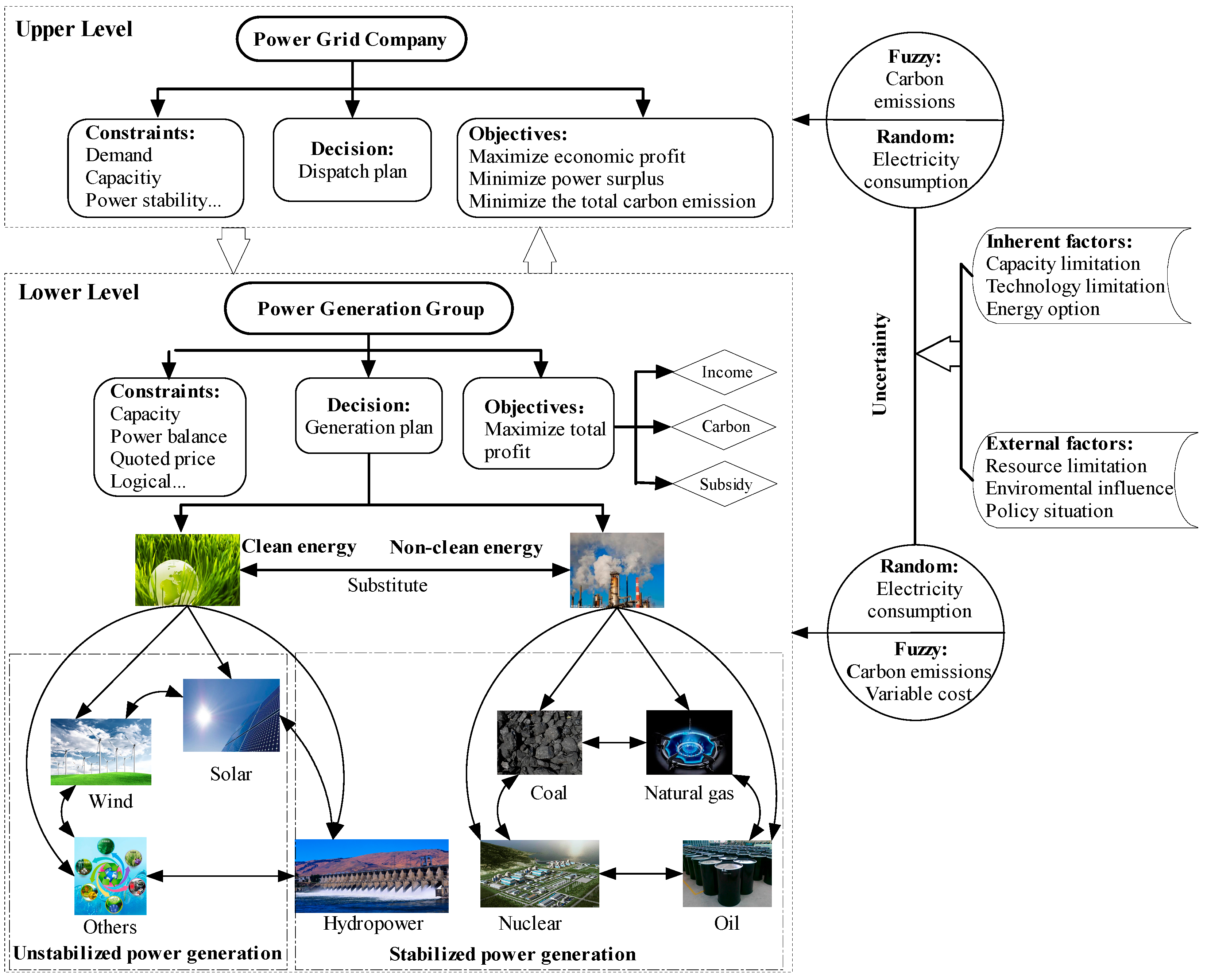
  • We establish a bi-level multi-objective model for a power dispatch problem which better reflects the real world. In the proposed model, the upper decision-maker is the regional power grid company and the lower decision-makers are the power generation groups.
  • We consider a hybrid uncertain environment, so use random and fuzzy variables to describe the imprecise information in the power dispatch problem.
  • We set the quoted power price and the power generation quantities as the decision variables to more accurately reflect the current power dispatch systems in many countries.
This paper has six sections. In the next section, the key power dispatch features are described. In Section 3, the mathematical model is established in detail. Two processes are introduced in Section 4 and the bi-level interactive solution method is proposed in Section 5. A case study is presented in Section 6 and conclusions are given in Section 7.

2. Problem Statement

In the power system, there are mainly two stakeholders: the power grid company and the power generation groups. For the upper level power grid company, determining an equitable dispatch plan for the power generation groups and determining the market power price are the key problems. For the lower level power generation groups, the power generation arrangement and setting the power price is important. Therefore, these two decision-makers have different objectives and constraints, so each is relatively independent. However, when the grid company makes a decision, the power generation group performances are of concern. At the same time, the power grid company decisions are a precondition for the power generation groups. In other words, these two decision makers have mutual influences and restrictions. Therefore, bi-level programming needs to be adopted to deal with the problem.
From the initial power dispatch to the end power generation process, there are several uncertainties. For example, as power consumption distribution can be determined from historical data, it is reasonable we use a random variable to describe electricity consumption. However, it is difficult to obtain a distribution for carbon emissions because of insufficient data, so it is necessary to employ a fuzzy variable to describe carbon emissions.
In summary, the uncertain bi-level power dispatch problem can be expressed as shown in Figure 1.

3. Modeling

In this section, an uncertain bi-level multi-objective power dispatch model will be established. The following notations are used.

3.1. Notations

The following notations are used to formulate the mathematical model.
Indices:
t : Time interval, t = 1 , 2 , 3 T ,
u : Consumption type, u = 1 , 2 , 3 U ,
g : Power generation group, g = 1 , 2 , 3 G ,
i : Power generation type, i = 1 , 2 , 3 I ,
j : Stabilized power generation type, j = 1 , 2 , 3 J .
Parameters:
d e m ¯ u t : Demand for consumption type u in time interval t , random variable,
o g , i , t : Operational cost for power grid company connecting power generation group g using generation type i in time interval t ,
a ˜ g , i : Carbon emissions produced by power generation group g using generation type i , fuzzy variable,
b t : Power grid company’s stand-by ratio in time interval t ,
S g , i , t : Capacity of power generation group g using generation type i in time interval t ,
v : Lower limit of stabilized power ratio,
p u l : Lowest unit power price for consumption type u ,
p u u : Highest unit power price for consumption type u ,
R i , t : Regional government subsidies for generation type i in time interval t ,
c ˜ g , i , t : Variable cost for power generation group g using generation type i in time interval t , fuzzy variable,
e g , t : Carbon emission allowances for power generation group g in time interval t ,
d : Unit price of carbon emission,
p i , t : Regional government controlled price for generation type i in time interval t .
Decision variables:
x g , t : Power generation quota dispatched to power generation group g in time interval t ,
x g , i , t : Power quantity generated by power generation group g using generation type i in time interval t ,
y u t : Unit market selling price for consumption type u in time interval t ,
y g , i , t : Unit quoted price at power generation group g using generation type i in time interval t .

3.2. Upper Level Dispatch Model

As the upper decision-maker, the power grid company needs to maximize total profits, guarantee power supply service stability and reduce environmental problems.

3.2.1. Upper Level Objectives

As a profit making organization, the power grid company first seeks to maximize profits, which can be described as the price difference between the power sales income and the purchase cost:
max F 1 = g = 1 G i = 1 I t = 1 T u = 1 U ( y u t d e m ¯ u t y g , i , t x g , i , t o g , i , t x g , i , t )
where t = 1 T u = 1 U y u t d e m ¯ u t is the power sales income for the power grid company, g = 1 G i = 1 I t = 1 T y g , i , t x g , i , t is the purchase cost, and g = 1 G i = 1 I t = 1 T o g , i , t x g , i , t is the operational cost.
Electricity cannot be stored, so the power grid company needs to balance supply and demand to minimize surplus power:
min F 2 = g = 1 G t = 1 T u = 1 U ( x g , t d e m ¯ u t )
where g = 1 G t = 1 T x g , t is total electricity generation, and t = 1 T u = 1 U d e m ¯ u t is the total electricity demand in the region.
Because of low carbon concerns, the power grid company seeks to minimize total carbon emissions:
min F 3 = g = 1 G i = 1 I t = 1 T a ˜ g , i x g , i , t
where g = 1 G i = 1 I t = 1 T a ˜ g , i x g , i , t is the total carbon emissions produced by all power generation groups.

3.2.2. Upper Level Constraints

Power demand constraint: the total power supply provided by the power grid company should satisfy the power consumption requirements.
u U t = 1 T d e m ¯ u t g = 1 G t = 1 T x g , t ,   t T
Stand-by power constraints: in case of emergency, the power grid company needs to set aside stand-by power capacity. Therefore, the total power dispatched to all power generation groups should be less than the available capacity of all generation groups.
g = 1 G x g , t ( 1 b t ) g = 1 G i = 1 I S g , i , t ,   t T
where g = 1 G x g , t is the total on-grid electricity quota to be dispatched to all power generation groups, and b t g = 1 G i = 1 I S g , i , t is the stand-by power capacity.
Power stability constraint: to ensure power supply stability, the power grid company may specify a lower limit for the stabilized power ratio.
g = 1 G j = 1 J x g , j , t / g = 1 G i = 1 I x g , i , t v ,   t T
where g = 1 G j = 1 J x g , j , t is the power available for the stabilized power generation types, and g = 1 G i = 1 I x g , i , t is the power available for all power generation types.
Power price constraint: the power market sales price y u t should be larger than the lowest price p u l and lower than the highest price p u u .
p u l y u t p u u
Logical constraint: the power supplied and the power sales price cannot be negative.
x g , t 0 , y u t 0 ,   g G , t T

3.3. Lower Level Generation Model

As the lower decision-makers, the power generation groups need to plan their respective power generation quantities and prices for all power generation types according to the power grid company’s dispatch plan.

3.3.1. Lower Level Objective

Each power generation group seeks to maximize its own profit, which is obtained from two different sources. The first source is the income received from selling power to the grid company plus government subsidies minus the total costs, which are made up of production variable costs, pollution treatment costs. The second source is the income received from carbon trading.
max f g = i = 1 I t = 1 T ( y g , i , t + R i , t c ˜ g , i , t ) x g , i , t + i = 1 I t = 1 T d ( e g , t a ˜ g , i x g , i , t )
where i = 1 I t = 1 T ( y g , i , t + R i , t ) x g , i , t is the total income, and i = 1 I t = 1 T c ˜ g , i , t x g , i , t is the total costs; i = 1 I t = 1 T d ( e g , t a ˜ g , i x g , i , t ) is the carbon trading income, when carbon emissions exceed emissions allowances, it is negative; conversely, when carbon emissions are less than emissions allowances, it is positive.

3.3.2. Lower Level Constraints

Capacity constraints: it is assumed that the capacity for power generation group g using type i in a certain time interval t can be determined by using historical data. For each power generation type in a power group, power generation should not exceed the corresponding capacity.
x g , i , t S g , i , t ,   g G , i I , t T
Balance constraints: the total power generated by the power generation group for all types should be equal to the power dispatched by the power grid company.
i = 1 I x g , i , t = x g , t , g G , t T
Generation constraint: the power generation group generates power only when the unit income is greater than the unit costs.
y g , i , t + R i , t c ˜ g , i , t , g G , i I , t T
where y g , i , t + R i , t is the unit income, and c ˜ g , i , t is the unit costs.
Quoted price constraint: the power generation group quoted price y g , i , t cannot be higher than the regional government controlled price p i , t .
y g , i , t p i , t , g G , i I , t T
Logical constraint: Equation (14) ensures non-negative variables.
x g , i , t , y g , i , t 0 , g G , i I , t T

4. Model Processing

As the model has the uncertain parameters d e m ¯ t , a ˜ g , i , c ˜ g , i , t , it needs to be further processed and transformed into a solvable model with mathematical meaning. For this, two approaches are proposed to handle the uncertain programming, as shown in Equations (1)–(14). The expected value model can produce a reference solution for the average meaning with no need for any parameter to be predetermined; therefore, this model can ease the decision-maker’s burden. The chance constrained model allows for plans to be adapted to different predetermined confidence levels depending on the situation.
The theorems to be used in this model are outlined first.
Theorem 1
[23] Given three normally distributed random variables ξ ~ N ( μ , σ 2 ) , ξ 1 ~ N ( μ 1 , σ 1 2 ) , ξ 2 ~ N ( μ 2 , σ 2 2 ) , where μ , μ 1 , μ 2 are the mean values, σ 2 , σ 1 2 , σ 2 2 are the variances, and σ , σ 1 , σ 2 are the standard deviations, we have:
(1)
P r { ξ x } α μ + σ Φ ( α ) 1 x ;
(2)
{ E ( ξ ) = μ ; E ( k ) = k E ( k ξ ) = k E ( ξ ) = k μ ;
(3)
a ξ 1 + b ξ 2 N ( a μ 1 + b μ 2 , a 2 σ 1 2 + b 2 σ 2 2 ) .
where k , a , b are real numbers, is a probability, E ( ξ ) is the expected value of the normal distribution random variable ξ , ξ μ σ is the standard normal distribution random variable, and Φ ( α ) 1 is the lower α quartile of the standard normal distribution such that P r ( ξ μ σ Φ ( α ) 1 ) = α .
Definition 1
[24] Let L ( · ) , R ( · ) be two reference functions. If the membership function of fuzzy variable ξ has the following form
μ ξ ( x ) = { L ( m x α ) , x m , α > 0 R ( x m β ) , x m , β > 0
then ξ is called an LR fuzzy variable denoted by ( m , α , β ) L R . L, R are the left and right branch of ξ , α , β are the left and right spread of ξ , and m is the central value of ξ . The γ -cut ( 0 γ 1 ) for the LR fuzzy variable is
ξ γ = [ ξ γ L , ξ γ R ] = [ m L 1 ( γ ) α , m + R 1 ( γ ) β ] , γ [ 0 , 1 ]
Theorem 2
[24] Given two LR fuzzy variables ξ 1 = ( m 1 , α 1 , β 1 ) L R and ξ 2 = ( m 2 , α 2 , β 2 ) L R , where m 1 , m 2 are the central values for ξ 1 , ξ 2 , and α 1 , α 2 and β 1 , β 2 are the left and right spreads for ξ 1 , ξ 2 . Then we have:
(1)
{ ξ 1 + ξ 2 = ( m 1 + m 2 , α 1 + α 2 , β 1 + β 2 ) L R ξ 1 ξ 2 = ( m 1 m 2 , α 1 + β 2 , β 1 + α 2 ) L R k ξ 1 = ( k m 1 , k α 1 , k β 1 ) L R , k > 0 ;
(2)
P o s { ξ 1 ξ 2 } γ m 1 γ R m 2 γ L ;
(3)
E [ ξ 1 ] = m 1 + β 1 α 1 4 ;
where k is a real number, γ ( 0 γ 1 ) and E [ ξ 1 ] are the possibility and expected values, m 1 γ R is the right end point for ξ 1 ’s γ -cut and m 2 γ L is the left end point for ξ 2 ’s γ -cut.

4.1. Chance Constrained Model

Since there are random parameters in objective functions (1) and (2), it is difficult to accurately determine the maximum profit or the minimum power surplus.
The following is proposed to deal with the objective functions. First, the decision-maker predetermines confidence levels γ 1 and γ 2 , then constructs chance constraints in which the objective functions are better than the ideal objective values F 1 and F 2 . At this point, the decision maker just needs to optimize the ideal objective values, as shown in Equations (15) and (16).
max F 1 s . t .   P r { g = 1 G i = 1 I t = 1 T u = 1 U ( y u t d e m ¯ u t y g , i , t x g , i , t o g , i , t x g , i , t ) F 1 } γ 1
indicating the probability that the power grid company’s profit g = 1 G i = 1 I t = 1 T u = 1 U ( y u t d e m ¯ u t y g , i , t x g , i , t o g , i , t x g , i , t ) is no less than the ideal value F 1 is larger than γ 1 .
min F 2 s . t .   P r { g = 1 G t = 1 T u = 1 U ( x g , t d e m ¯ u t ) F 2 } γ 2
where γ 2 is the confidence level, indicating that the probability that the gap between supply and demand g = 1 G t = 1 T u = 1 U ( x g , t d e m ¯ u t ) is no more than the ideal value F 2 is larger than γ 2 .
Based on Theorem 1, Equations (15) and (16) can be equivalently transformed into Equations (17) and (18), respectively.
max F 1 F 1 + g = 1 G i = 1 I t = 1 T u U ( y g , i , t + o g , i , t ) x g , i , t g = 1 G i = 1 I t = 1 T u = 1 U y u t μ d e m u t Φ ( 1 γ 1 ) 1 g = 1 G i = 1 I t = 1 T u U y u t 2 σ d e m u t 2
where Φ ( 1 γ 1 ) 1 is the lower 1 γ 1 quartile of the standard normal distribution.
min F 2 g = 1 G t = 1 T x g , t F 2 + u = 1 U t = 1 T μ d e m u t + Φ ( 1 γ 2 ) 1 u = 1 U t = 1 T σ d e m u t 2
where Φ ( 1 γ 2 ) 1 is the lower 1 γ 2 quartile of the standard normal distribution.
We can use a similar approach to handle the objective functions with fuzzy variables. Equations (3) and (9) are then replaced with Equations (19) and (20).
min F 3 s . t .   P o s { g = 1 G i = 1 I t = 1 T a ˜ g , i x g , i , t F 3 } γ 3
indicating the possibility that the carbon emission g = 1 G i = 1 I t = 1 T a ˜ g , i x g , i , t is no more than the ideal value F 3 is larger than confidence level γ 3 .
max f g s . t .   P o s [ i = 1 I t = 1 T ( y g , i , t + R i , t c ˜ g , i , t ) x g , i , t + i = 1 I t = 1 T d ( e g , t a ˜ g , i x g , i , t ) f g ] γ 5
indicating that each power generation group’s profit i = 1 I t = 1 T ( y g , i , t + R i , t c ˜ g , i , t ) x g , i , t + i = 1 I t = 1 T d ( e g , t a ˜ g , i x g , i , t ) is no less than the ideal value f g with the possibility γ 5 .
Based on Theorem 2, Equations (19) and (20) can be transformed into Equations (21) and (22).
min F 3 i = 1 I t = 1 T a g , i x g , i , t i = 1 I t = 1 T α e g , i x g , i , t ( 1 γ 3 ) F 3
max f g t = 1 T i = 1 I [ ( y g , i , t + R i , t c g , i , t d a g , i ) x g , i , t + d e g , t ] + ( 1 γ 5 ) t = 1 T i = 1 I ( α c g , i , t + d α a g , i ) x g , i , t f g
Also, Constraints (4) and (12) can be transformed into Equations (23) and (24).
P r { u U t = 1 T d e m ¯ u t g = 1 G t = 1 T x g , t } γ 4
the probability that the power consumption u U t = 1 T d e m ¯ u t is lower than or equal to the power supply from the power grid company g = 1 G t = 1 T x g , t is larger than γ 4 .
P o s { y g , i , t + R i , t c ˜ g , i , t } γ 6
indicating that the income y g , i , t + R i , t is greater than the costs c ˜ g , i , t for any g , i , t under the confidence level γ 6 .
Based on Theorem 1, Equation (23) can be equivalently converted into Equation (25).
g = 1 G t = 1 T x g , t u = 1 U t = 1 T μ d e m u t + Φ ( γ 4 ) 1 u = 1 U t = 1 T σ d e m u t 2 ,   t T
where Φ ( γ 4 ) 1 is the lower γ 4 quartile of the standard normal distribution.
And based on Theorem 2, constraint (24) is equivalent to Equation (26).
c g , i , t ( 1 γ 6 ) α c g , i , t y g , i , t + R i , t , g G , i I , t T
Considering the above, the following Model (27) is the equivalent chance constrained model:
max F 1 min F 2 min F 3 s . t . { F 1 + g = 1 G i = 1 I t = 1 T u U ( y g , i , t + o g , i , t ) x g , i , t g = 1 G i = 1 I t = 1 T u = 1 U y u t μ d e m u t Φ ( 1 γ 1 ) 1 g = 1 G i = 1 I t = 1 T u U y u t 2 σ d e m u t 2 g = 1 G t = 1 T x g , t F 2 + u = 1 U t = 1 T μ d e m t + Φ ( 1 γ 2 ) 1 u = 1 U t = 1 T σ d e m t 2 i = 1 I t = 1 T a g , i x g , i , t i = 1 I t = 1 T α e g , i x g , i , t ( 1 γ 3 ) F 3 g = 1 G t = 1 T x g , t u = 1 U t = 1 T μ d e m u t + Φ ( γ 4 ) 1 u = 1 U t = 1 T σ d e m u t 2 ,   t T g = 1 G i = 1 I b t S g , i , t + g = 1 G x g , t g = 1 G i = 1 I S g , i , t ,   t T g = 1 G j = 1 J x g , j , t / g = 1 G i = 1 I x g , i , t v ,   t T p u l y u t p u u x g , t 0 , y u t 0 , g G , t T max f g s . t . { t = 1 T i = 1 I [ ( y g , i , t + R i , t c g , i , t d a g , i ) x g , i , t + d e g , t ] + ( 1 γ 5 ) t = 1 T i = 1 I ( α c g , i , t + d α a g , i ) x g , i , t f g x g , i , t S g , i , t ,   g G , i I , t T i = 1 I x g , i , t = x g , t , g G , t T c g , i , t ( 1 γ 6 ) α c g , i , t y g , i , t + R i , t , g G , i I , t T y g , i , t p i , t , g G , i I , t T x g , i , t , y g , i , t 0 , g G , i I , t T

4.2. Expected Value Model

For the bi-level model proposed in Section 3, we can also optimize the expected objectives subject to the expected constraints. Based on Theorem 1 and Theorem 2, Equations (1)–(3) and (9) can be transformed into Equations (28)–(31), respectively.
max F 1 = g = 1 G i = 1 I t = 1 T u = 1 U ( y u t μ d e m u t ( y g , i , t + o g , i , t ) x g , i , t )
min F 2 = g = 1 G t = 1 T u = 1 U ( x g , t μ d e m u t )
min F 3 = g = 1 G i = 1 I t = 1 T ( a g , i + β a g , i α a g , i 4 ) x g , i , t
max f g = t = 1 T i = 1 I [ ( y g , i , t + R i , t c g , i , t d a g , i ) x g , i , t + d e g , t ] + ( α c g , i , t + d α a g , i β c g , i , t d β a g , i 4 ) x g , i , t
where μ d e m u t is the mean value of the random variables d e m ¯ u t ; a g , i , α a g , i , β a g , i are the central value and left and right spreads of a ˜ g , i ; and c g , i , t , α c g , i , t and β c g , i , t are the central value, left and right spreads of c ˜ g , i , t .
Similarly, Constraints (4) and (12) can be transformed into Equations (32) and (33).
u = 1 U t = 1 T μ d e m u t g = 1 G t = 1 T x g , t ,   t T
y g , i , t + R i , t c g , i , t + β c g , i , t α c g , i , t 4 , g G , i I , t T
Therefore, the equivalent expected value model is obtained, as shown in Equation (34):
max F 1 = g = 1 G i = 1 I t = 1 T u = 1 U ( y u t μ d e m u t ( y g , i , t + o g , i , t ) x g , i , t ) min F 2 = g = 1 G t = 1 T u = 1 U ( x g , t μ d e m u t ) min F 3 = g = 1 G i = 1 I t = 1 T ( a g , i + β a g , i α a g , i 4 ) x g , i , t s . t . { u = 1 U t = 1 T μ d e m u t g = 1 G t = 1 T x g , t ,   t T g = 1 G i = 1 I b t S g , i , t + g = 1 G x g , t g = 1 G i = 1 I S g , i , t ,   t T g = 1 G j = 1 J x g , j , t / g = 1 G i = 1 I x g , i , t v ,   t T p u l y u t p u u x g , t 0 , y u t 0 , g G , t T max f g = t = 1 T i = 1 I [ ( y g , i , t + R i , t c g , i , t d a g , i ) x g , i , t + d e g , t ] + ( α c g , i , t + d α a g , i β c g , i , t d β a g , i 4 ) x g , i , t s . t . { x g , i , t S g , i , t ,   g G , i I , t T i = 1 I x g , i , t = x g , t , g G , t T y g , i , t + R i , t c g , i , t + β c g , i , t α c g , i , t 4 , g G , i I , t T y g , i , t p i , t , g G , i I , t T x g , i , t , y g , i , t 0 , g G , i I , t T

5. Solution Method

The bi-level multi-objective programming has always been a difficult NP problem, it is usually solved using Stackelberg solution. However, Stackelberg solution is suitable for the situation where two sides are not cooperating with each other. In the above models, there exists a cooperative motive between the upper and lower level decision makers. In order to resolve these conflicts of interest, the upper and lower level decision makers can interact with a certain degree of satisfaction. Therefore, this paper uses the interactive solution method based on satisfaction degree (SD) to solve Models (27) and (34), the detailed steps are as follows:

5.1. Eliciting the Satisfaction Degree Functions

To obtain the satisfaction degree functions for the objectives, membership functions for the objective functions are employed.
Assume Equations (35)–(38) are the minimum values for the objective functions:
F 1 min = min { F 1 ( x , y ) | ( x , y ) Q }
F 2 min = min { F 2 ( x , y ) | ( x , y ) Q }
F 3 min = min { F 3 ( x , y ) | ( x , y ) Q }
f g min = min { f g ( x , y ) | ( x , y ) Q }
where g = 1 , 2 , , G , and Q is the feasible region which constructed by all the constraints in both the upper and the lower level.
Assume Equations (39)–(42) are the maximum values for the objective functions:
F 1 max = max { F 1 ( x , y ) | ( x , y ) Q }
F 2 max = max { F 2 ( x , y ) | ( x , y ) Q }
F 3 max = max { F 3 ( x , y ) | ( x , y ) Q }
f g max = max { f g ( x , y ) | ( x , y ) Q }
Then, the linear satisfaction functions (43)–(45) are employed to characterize the objective functions on the upper level.
S D 0 ( F 1 ( x , y ) ) = { 1 F 1 ( x , y ) F 1 max F 1 ( x , y ) F 1 min F 1 max F 1 min F 1 min < F 1 ( x , y ) F 1 max 0 F 1 ( x , y ) < F 1 min
S D 0 ( F 2 ( x , y ) ) = { 1 F 2 ( x , y ) F 2 min F 2 max F 2 ( x , y ) F 2 max F 2 min F 2 min < F 2 ( x , y ) F 2 max 0 F 2 ( x , y ) > F 2 max
S D 0 ( F 3 ( x , y ) ) = { 1 F 3 ( x , y ) F 3 min F 3 max F 3 ( x , y ) F 3 max F 3 min F 3 min < F 3 ( x , y ) F 3 max 0 F 3 ( x , y ) > F 3 max
The lower level satisfaction functions are defined as follows:
S D g ( f g ( x , y ) ) = { 1 f g ( x , y ) f g max f g ( x , y ) f g min f g max f g min f g min < f g ( x , y ) f g max 0 f g ( x , y ) < f g min
Note that the satisfaction degrees are in the interval [0, 1].

5.2. Evaluating the Satisfactorysolution

After determining the satisfaction functions on the two levels, the upper level decision-maker first determines minimum acceptable satisfaction degrees λ 0 1 , λ 0 2 , λ 0 3 [ 0 , 1 ] ; in this way, the upper level objectives can be converted into the constraints in Model (47). Then, the lower level satisfaction degree is maximized,
max   λ s . t . { S D 0 ( F 1 ( x , y ) ) λ 0 1 S D 0 ( F 2 ( x , y ) ) λ 0 2 S D 0 ( F 3 ( x , y ) ) λ 0 3 S D g ( f g ( x , y ) ) λ , g = 1 , 2 , G ( x , y ) Q
where λ is the assistant variable.
Assume that the optimal solution for the Model (47) is X = ( x * , y * , λ * ) ; then, the following two methods can be used to determine whether it is a satisfactory solution to the bi-level model:
(1) Satisfaction degree for the lower level
If S D g ( f g ( x * , y * ) ) λ g ( λ g is the minimum acceptable satisfaction degree predetermined by each power generation group) holds for all g = 1 , 2 , G , then X = ( x * , y * , λ * ) can be accepted as the satisfactory solution to the bi-level problem; otherwise, the upper level decision maker must reduce its acceptable satisfaction degree, in order to increase the satisfaction degrees for the lower level decision makers.
(2) Balancing the satisfaction degree between the upper level and lower levels
To evaluate the overall satisfaction degree on the upper level, the weighted sum method is used to evaluate the satisfaction degree for the three upper level objective functions, as shown in Equation (48),
S D ¯ = h = 1 3 w 0 h S D 0 ( F h ( X ) ) 3
where w 0 1 , w 0 2 , w 0 3 ( h = 1 3 w 0 h = 1 , w 0 h 0 ) are the weights for the three objectives in the upper level.
Equanimity between the upper level and the lower level is the basis of healthy development. The upper level decision-maker needs to treat each lower level decision-maker equally. Therefore, the ratio of satisfaction degree between the upper and lower levels can be used to balance the satisfaction degree, so the satisfaction ratio is:
Δ = min g G S D g ( f g ( X ) ) / S D ¯ = 3 min g G S D g ( f g ( X ) ) / h = 1 3 w 0 h S D 0 ( F h ( X ) )
Let Δ u and Δ l be the upper and lower bounds of Δ .
There are two scenarios in which the acceptable satisfaction degrees need to be adjusted: (1) When Δ > Δ u , the upper level decision maker needs to increase its acceptable satisfaction degree λ 0 h ( h = 1 , 2 , 3 ) ; (2) When Δ < Δ l , the upper level decision-maker needs to decrease the acceptable satisfaction degree to improve the satisfaction degrees of the lower level decision-makers.
If the optimal solution X = ( x * , y * , λ * ) of the model meets the above requirements, then the solution can be considered a satisfactory solution to the bi-level problem.

6. Case Study

A case study based on China power system is now presented to verify the validity of the proposed model.

6.1. Related Data

A region has five power generation groups, within which there are four generation types; i = 1 : fire power, i = 2 : hydropower, i = 3 : wind power, i = 4 : solar power.
We assume that the installed capacity S g , i , t , variable costs c ˜ g , i , t , government subsidies R i , t , and the regional government controlled price p i , t do not change in the considered period t = 1, 2, 3. The detailed parameters are shown in Table 1 and Table 2.
In this case, the operational costs for the power grid company connecting the power generation groups are assumed to be the same, and thus can be omitted. The other parameters related to the power grid company are listed in Table 3.

6.2. Results

6.2.1. Results of the Chance Constrained Model

We used the chance constrained Model (27) and set the decision-makers’ confidence levels for the upper and lower level chance constraints as 0.9; i.e., γ 1 = γ 2 = γ 3 = γ 4 = γ 5 = γ 6 = 0.9 ; then the following steps are taken to determine the solution:
Step 1: We use LINGO to solve Equations (35) and (39) to respectively obtain the minimum and maximum values for the objective function F 1 . The minimum value is 16.10664 million CNY and the maximum value is 1053.504 million CNY. Similarly, the rest of the objectives’ minimum and maximum values are determined, the detailed results for which are shown in Table 4.
Step 2: We use Equations (43)–(46) to obtain the linear satisfaction functions:
S D 0 ( F 1 ( x , y ) ) = { 1 F 1 ( x , y ) 1053.504 F 1 ( x , y ) 16.10664 1053.504 16.10664 16.10664 < F 1 ( x , y ) 1053.504 0 F 1 ( x , y ) < 16.10664 , S D 0 ( F 2 ( x , y ) ) = { 1 F 2 ( x , y ) 106.3082 578.523 F 2 ( x , y ) 578.523 106.3082 106.3082 < F 2 ( x , y ) 578.523 0 F 2 ( x , y ) > 578.523
S D 0 ( F 3 ( x , y ) ) = { 1 F 3 ( x , y ) 2461995 2991382 F 3 ( x , y ) 2991382 2461995 2461995 < F 3 ( x , y ) 2991382 0 F 3 ( x , y ) > 2991382 , S D 1 ( f 1 ( x , y ) ) = { 1 f 1 ( x , y ) 55.98099 f 1 ( x , y ) 0.002862 55.98099 0.002862 0.002862 < f 1 ( x , y ) 55.98099 0 f 1 ( x , y ) < 0.002862
S D 2 ( f 2 ( x , y ) ) = { 1 f 2 ( x , y ) 57.35391 f 2 ( x , y ) 0.002436 57.35391 0.002436 0.002436 < f 2 ( x , y ) 57.35391 0 f 2 ( x , y ) < 0.002436 , S D 3 ( f 3 ( x , y ) ) = { 1 f 3 ( x , y ) 125.478 f 3 ( x , y ) 0.563342 125.478 0.563342 0.563342 < f 3 ( x , y ) 125.478 0 f 3 ( x , y ) < 0.563342
S D 4 ( f 4 ( x , y ) ) = { 1 f 4 ( x , y ) 70.68472 f 4 ( x , y ) 0.219078 70.68472 0.219078 0.219078 < f 4 ( x , y ) 70.68472 0 f 4 ( x , y ) < 0.219078 , S D 5 ( f 5 ( x , y ) ) = { 1 f 5 ( x , y ) 98.7799 f 5 ( x , y ) 0.002097 98.7799 0.002097 0.002097 < f 5 ( x , y ) 98.7799 0 f 5 ( x , y ) < 0.002097
Step 3: When the upper level decision-makers’ satisfaction degree for all three objectives are 0.9, Model (47) is used to determine the optimization results. The minimum satisfaction degree for the lower level decision-makers is 0.343, the ratio of the upper and lower level’s satisfaction degree is 0.382 and the power grid profit is 949.7642 million CNY. Power generation group No. 1 needs to generate 171.168 million kWh in the first time interval, 111.3167 million kWh in the second time interval and 105.8273 million kWh in the third time interval. The detailed optimization results and objective values are shown in Table 5, Table 6 and Table 7.

6.2.2. Results of the Expected Value Model

The expected value Model (34) is also used to solve the problem. When the upper decision-makers’ acceptable satisfaction degree for each of the three objectives is 0.9, the minimal satisfaction degree for the lower level decision-makers is 0.343, the ratio between the upper and lower level’s satisfaction degree is 0.381, and the power grid profit is 999.390 million CNY. In this case, power generation group No. 1 needs to generate 147.7927 million kWh in the first time interval, 58.38397 million kWh in the second time interval, and 50.24306 million kWh in the third time interval. The detailed objective values and optimization results are shown in Table 8, Table 9 and Table 10.

6.3. Comparison and Discussion

In this section, three comparisons are given; the first is based on the satisfaction degree, the second based on the confidence level and the third is a comparison between the chance constrained model and the expected value model.
(1) Comparison based on different satisfaction degrees
When the decision-makers’ confidence levels on the upper and lower level chance constraints are set at 0.9, by changing the upper decision-makers’ satisfaction degrees for the three objectives simultaneously, Model (47) can be used to determine the optimization results under different satisfaction degrees. When the satisfaction degrees are all 0.75, the minimum satisfaction degree for the lower level decision-makers is 0.730, the ratio of the upper and lower level’s satisfaction degree is 0.973, and the power grid profit is 794.1546 million CNY. The detailed objective values are shown in Table 11.
From the optimization results in Table 11, it can be seen that with a fixed confidence level, a higher upper level satisfaction degree can significantly reduce the lower level satisfaction degrees, as shown in Figure 2. This is because when the upper level satisfaction rises, the conflicts between the two decision-making levels are more intense, so the feasible region on the lower level is narrowed. Therefore, choosing a suitable satisfaction degree is very important.
(2) Comparison based on different confidence levels
The upper level satisfaction degrees for the three objectives are set at 0.9, which means λ 0 1 = λ 0 2 = λ 0 3 = 0.9 .However, if confidence levels are changed, the results shown in Table 12 are obtained. When the confidence level is set to 0.6, the satisfaction degrees on the upper and lower levels are 0.9 and 0.334, respectively, the ratio between the upper and lower level satisfaction degrees is 0.371, and the power grid company profit is 993.495 million CNY. The detailed objective values are shown in Table 12.
From the results of Table 12, it can be seen that with a fixed satisfaction degree, as the confidence level declines, better objectives can be achieved, as shown in Figure 3. This is because a lower confidence level means there is a larger feasible decision region for all decision-makers, which could lead to better results; however, it comes with higher uncertainty.
(3) Comparison between the chance constrained model and the expected value model
According to Table 8 and Table 11, we can draw Figure 3, which shows the results of the chance constrained model and the expected value model: (a) and (b) present the power grid company’s profit and the total carbon emissions. It can be seen that the objective values in the chance constrained model and the expected value model intersect.
Therefore, it can be concluded that the result of the expected value model is equal to that of the chance constrained model under a certain confidence level. By solving the chance constrained model, a series of results can be obtained. Different decisions can be given by decision-makers with varying confidence levels.
(4) Comparison based on different carbon emission reduction policies
In the following, we compare the result under the carbon trading policy to that under the carbon limit policy.
For a power generation group under the carbon trading policy, there are two sources of income, the first is the income brought by power market, and the second is the income from the carbon trading market, therefore, Equation (9) is built as the objective. However, when we consider the same problem under the carbon limit policy, a different bi-level model should be established. Since these policies mainly impact the power generation groups, and have little effect on the situation of the power grid company, the upper level model will be unchanged, but the lower level model should be rebuilt, and the details are as follows.
Under the carbon limit policy, each power generation group has to meet a constraint of carbon emission limit as shown in Equation (49),
i = 1 I a ˜ g , i x g , i , t e g , t ,   g G , t T
and meanwhile, the objective function should be
max f g = i = 1 I t = 1 T ( y g , i , t + R i , t c ˜ g , i , t e g , i ) x g , i , t
where the income is only from the power market.
We use the similar chance constrained operator to handle the above Equations (49) and (50), and can get the following crisp equivalent model (51) for the lower level power generation groups under the carbon limit policy.
max   f g s . t . { t = 1 T i = 1 I ( y g , i , t + R i , t e g , i c g , i , t ) x g , i , t + ( 1 γ 7 ) t = 1 T i = 1 I α c g , i , t x g , i , t f g i = 1 I a g , i x g , i , t ( 1 γ 8 ) i = 1 I α e g , i x g , i , t e g , t ,   g G , t T x g , i , t S g , i , t ,   g G , i I , t T i = 1 I x g , i , t = x g , t , g G , t T c g , i , t ( 1 γ 6 ) α c g , i , t y g , i , t + R i , t e g , i , g G , i I , t T y g , i , t p i , t , g G , i I , t T x g , i , t , y g , i , t 0 , g G , i I , t T
where confidence levels γ 7 and γ 8 are predetermined.
In the above Section 6.2.1, we have obtained the results under the carbon trading policy. In the following, the confidence levels and satisfaction degrees are all set at 0.9, which are the same as that in Section 6.2.1. Then after solving the bi-level model with lower level Model (51), the second column of Table 13 is derived to describe the decision results under the carbon limit policy.
From Table 13, it can be found that the total carbon emission and the power generation groups' profits are all increased when the carbon limit policy is replaced by the carbon trading policy. However, it is worth noting that the profit growth rates are far higher than the carbon emission growth rate. More specifically, through carbon trading policy, carbon allowance will be used to a more great extent; and the part beyond the carbon emission limit will bring extra economic benefits in an even more effective way. In this way, the more environmentally friendly power generation group has more advantages. Based on the above discussion, a conclusion can be produced: setting severe carbon allowance and allowing carbon trading will have a great significance in realizing sustainable development of power industry.

7. Conclusions

This study investigated a low carbon based power dispatch problem under an uncertain environment and proposed an efficient, powerful bi-level multi-objective decision-making model with carbon related objectives. In the proposed model, the power grid company is the upper level decision-maker who decides on the power dispatch plan, and the power generation groups are the lower level decision-makers who decide on the generation plan. As there are random and fuzzy parameters in the proposed model, two methods are introduced to construct a chance constrained model and an expected value model. Then, based on random and fuzzy theories, we equivalently transformed these into crisp models and the models were converted into single level models using the satisfaction method. A case study and comparative analysis were given to validate the efficiency of the proposed approach.
Based on this process, the following conclusions can be made.
(1)
As all action is based on the power demand estimation, the power grid company needs to have enhanced forecasting abilities.
(2)
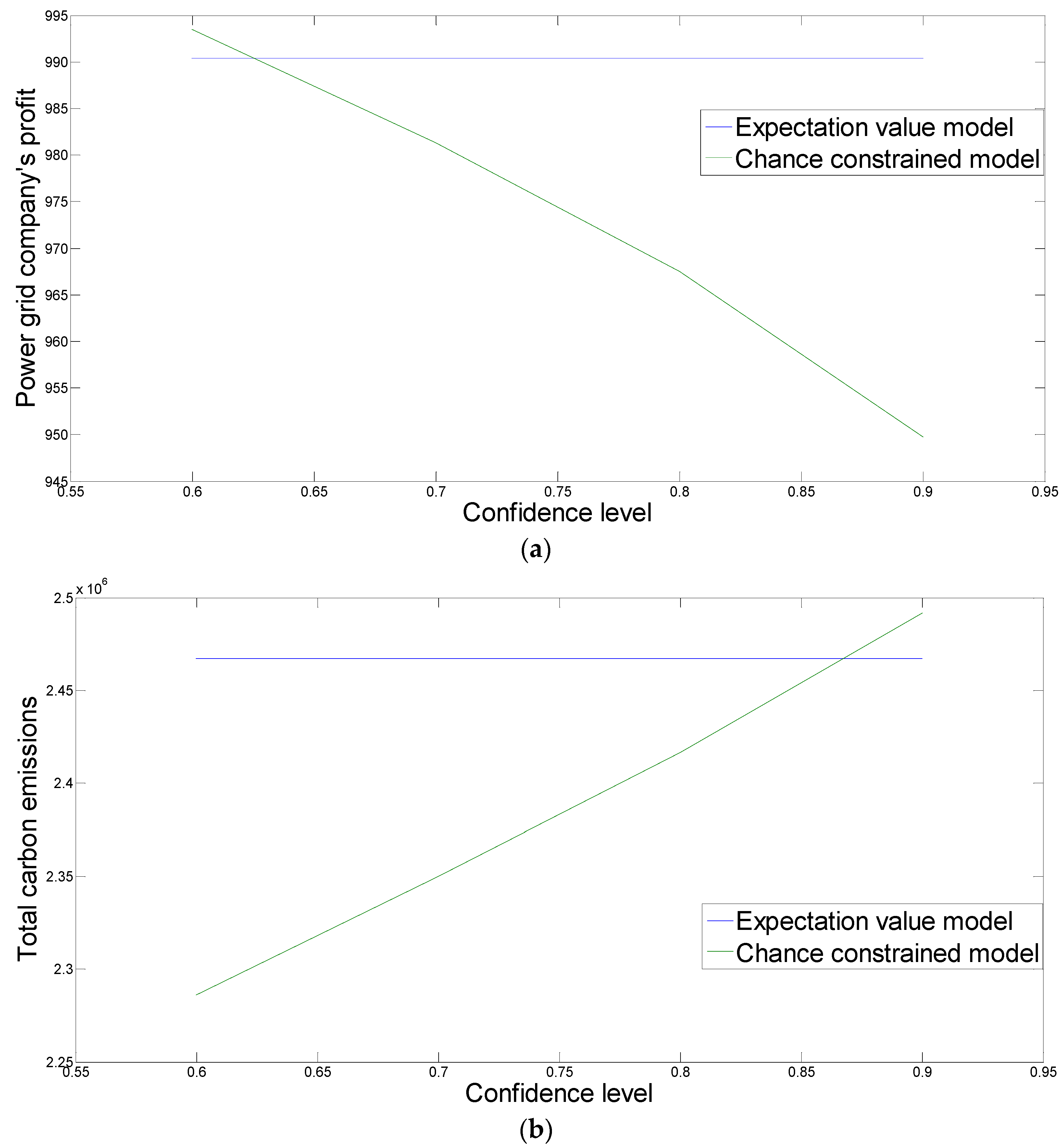
The chance constrained model and the expected value model are suitable for different decision making scenarios. The expected value model can give a reference solution for an average situation and the chance constrained model can suggest a range of plans depending on the confidence levels.
(3)
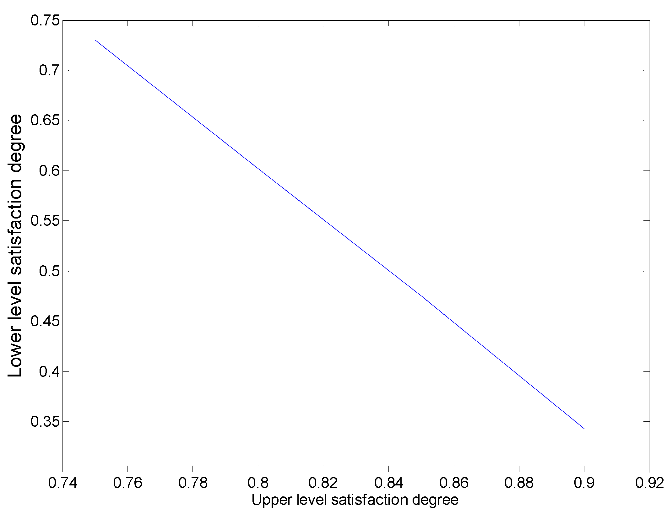
Upper level decision makers need to carefully consider all factors to determine the satisfaction degree so as to balance the interests between all decision making levels.
(4)
Severe carbon allowance and carbon trading will have a great significance in realizing sustainable development of power industry.

Acknowledgements

We thank those that have given constructive comments and feedback to help improve this paper. Supported was provided by the National Natural Science Foundation of China (Grant Nos. 71401093, 71473155), China Scholarship Council (Grant No. 201606875006), Soft Science Research Project of Shaanxi Province (Grant No. 2016KRM089), Research Center for Systems Science & Enterprise Development (Grant No. Xq16B01) and the Fundamental Research Funds for the Central Universities (Grant No. 14SZYB08).

Author Contributions

Xiaoyang Zhou designed the model and performed the experiments. Jian Chai and Kin Keung Lai collected the data; Benjamin Lev contributed analysis tools; and Canhui Zhao wrote the paper.

Conflicts of Interest

The authors declare no conflict of interest.

References

  1. Gao, C.; Li, Y. Evolution of China’s power dispatch principle and the new energy saving power dispatch policy. Energy Policy 2010, 38, 7346–7357. [Google Scholar]
  2. Gao, Y.; Cheng, H.; Zhu, J.; Liang, H.; Li, P. The optimal dispatch of a power system containing virtual power plants under fog and haze weather. Sustainability 2016, 8, 1–22. [Google Scholar] [CrossRef]
  3. Niknam, T.; Firouzi, B.B.; Mojarrad, H.D. A new evolutionary algorithm for non-linear economic dispatch. Expert Syst. Appl. 2011, 38, 13301–13309. [Google Scholar] [CrossRef]
  4. Pruitt, K.A.; Leyffer, S.; Newman, A.M.; Braun, R.J. A mixed-integer nonlinear program for the optimal design and dispatch of distributed generation systems. Optim. Eng. 2014, 15, 167–197. [Google Scholar] [CrossRef]
  5. Barcelo, W.R.; Rastgoufard, P. Dynamic economic dispatch using the extend security constrained economic dispatch algorithm. IEEE Trans. Power Syst. 1997, 12, 961–967. [Google Scholar] [CrossRef]
  6. Panigrahi, C.K.; Chattopadhyay, P.K.; Chakrabarti, R.N.; Basu, M. Simulated annealing technique for dynamic economic dispatch. Electr. Power Compon. Syst. 2006, 34, 577–586. [Google Scholar] [CrossRef]
  7. Dos Santos, C.L.; Mariani, V.C. Combining of chaotic differential evolution and quadratic programming for economic dispatch optimization with valve-point effect. IEEE Trans. Power Syst. 2006, 21, 989–996. [Google Scholar] [CrossRef]
  8. Faísca, N.P.; Rustem, B.; Dua, V. Bilevel and multilevel programming; Wiley-VCH: Weinheim, German, 2007. [Google Scholar]
  9. Hetzer, J.; Yu, D.C.; Bhattarai, K. An economic dispatch model incorporating wind power. IEEE Trans. Energy Convers. 2008, 23, 603–611. [Google Scholar] [CrossRef]
  10. Wierzbowski, M.; Lyzwa, W.; Musial, I. MILP model for long-term energy mix planning with consideration of power system reserves. Appl. Energy 2016, 169, 93–111. [Google Scholar] [CrossRef]
  11. Tan, Q.; Huang, G.H.; Cai, Y.P. A fuzzy evacuation management model oriented toward the mitigation of emissions. J. Environ. Inform. 2015, 25, 117–125. [Google Scholar] [CrossRef]
  12. Shen, Z.Y.; Chen, L.; Liao, Q. Effect of rainfall measurement errors on nonpoint-source pollution model uncertainty. J. Environ. Inform. 2015, 26, 14–26. [Google Scholar]
  13. Kockar, I.; Conejo, A.J.; Mcdonald, J.R. Influence of the emissions trading scheme on generation scheduling. Int. J. Electr. Power 2009, 31, 465–473. [Google Scholar] [CrossRef]
  14. Zhang, R.; Zhou, J.; Mo, L.; Ouyang, S.; Liao, X. Economic environmental dispatch using an enhanced multi-objective cultural algorithm. Electr. Power Syst. Res. 2013, 99, 18–29. [Google Scholar] [CrossRef]
  15. Chen, F.; Huang, G.H.; Fan, Y.R.; Liao, R.F. A nonlinear fractional programming approach for environmental–economic power dispatch. Int. J. Electr. Power Energy Syst. 2016, 78, 463–469. [Google Scholar] [CrossRef]
  16. Zhang, X.; Ren, X.; Zhong, J. The Comprehensive Evaluation Model of Low Carbon Benefits of the Power Planning and Its Application; Atlantis Press: Amsterdam, The Netherlands, 2015. [Google Scholar]
  17. Xu, J.; Yang, X.; Tao, Z. A tripartite equilibrium for carbon emission allowance allocation in the power-supply industry. Energy Policy 2015, 82, 62–80. [Google Scholar] [CrossRef]
  18. Zhu, Y.; Li, Y.P.; Huang, G.H.; Fan, Y.R.; Nie, S. A dynamic model to optimize municipal electric power systems by considering carbon emission trading under uncertainty. Energy 2015, 88, 636–649. [Google Scholar] [CrossRef]
  19. Heinricha, G.; Howellsb, M.; Bassona, L.; Petrie, J. Electricity supply industry modeling for multiple objectives under demand growth uncertainty. Energy 2007, 32, 2210–2229. [Google Scholar] [CrossRef]
  20. Hong, Y.Y.; Lin, J.K. Interactive multi-objective active power scheduling considering uncertain renewable energies using adaptive chaos clonal evolutionary programming. Energy 2013, 53, 212–220. [Google Scholar] [CrossRef]
  21. Zeng, Z.; Nasri, E.; Chini, A.; Ries, R.; Xu, J. A multiple objective decision making model for energy generation portfolio under fuzzy uncertainty: Case study of large scale investor-owned utilities in Florida. Renew. Energy 2015, 75, 224–242. [Google Scholar] [CrossRef]
  22. Zhou, Y.; Li, Y.P.; Huang, G.H. A robust possibilistic mixed-integer programming method for planning municipal electric power systems. Int. J. Electr. Power 2015, 73, 757–772. [Google Scholar] [CrossRef]
  23. Xu, J.; Yao, L. Random-Like Multiple Objective Decision Making; Springer Science & Business Media: Berlin, German, 2011. [Google Scholar]
  24. Xu, J.; Zhou, X. Fuzzy-Like Multiple Objective Decision Making; Springer: Berlin, German, 2011. [Google Scholar]
Figure 1. Uncertain bi-level power dispatching problem.
Sustainability 08 00533 g001
Figure 2. Satisfaction degree trade-off between the upper and the lower levels.
Sustainability 08 00533 g002
Figure 3. Objective values under the chance constrained model and the expected value model. (a) the power grid company’s profit; (b) the total carbon emissions.
Sustainability 08 00533 g003
Table 1. The parameters for the power generation group.
ParameterInstalled CapacityVariable CostsCarbon EmissionsGovernment SubsidiesGovernment Controlled Price
Index
g = 1i = 1158,760(0.24,0.037,0.01)(0.98,0.1,0.1)0.010.3346
i = 312,4080.500.380.6
i = 44500.800.420.88
g = 2i = 1136,080(0.24,0.037,0.01)(0.98,0.1,0.1)0.010.3346
i = 28560.50.09000.27
i = 314,2560.500.380.6
i = 4750.800.420.88
g = 3i = 1386,370(0.23,0.047,0.01)(0.98,0.26,0.26)0.010.3346
i = 226,3250.09000.27
i = 347520.500.380.6
g = 4i = 1238,680(0.23,0.037,0.01)(0.98,0.2,0.2)0.010.3346
i = 348000.500.380.6
i = 4750.800.420.88
g = 5i = 1116,910(0.24,0.037,0.01)(0.98,0.1,0.1)0.010.3346
i = 2108,868.50.09000.27
i = 323760.500.380.6
i = 460000.800.420.88
Table 2. The power consumption parameters.
ParameterDemandLowest Power PriceHighest Power Price
Index
u = 1t = 1N(27,900, 3800)0.410.5088
t = 2N(30,350, 1850)0.410.5088
t = 3N(35,200, 3600)0.410.5088
u = 2t = 1N(748,650, 11,250)0.410.5539
t = 2N(518,900, 8700)0.410.5539
t = 3N(636,700, 14,800)0.410.5539
u = 3t = 1N(208,250, 4650)0.410.7934
t = 2N(164,750, 9850)0.410.7934
t = 3N(158,550, 7150)0.410.7934
u = 4t = 1N(195,050, 4500)0.410.4983
t = 2N(164,850, 16,850)0.410.4983
t = 3N(175,350, 4250)0.410.4983
Table 3. The parameters for the power grid company.
ParameterCarbon Emissions AllowancesStorage RatioStabilized Power RatioPrice of Carbon Emissions Rights
Index g = 1g = 2g = 3g = 4g = 5
Tt = 1177,367152,028431,653266,653130,6120.020.70.03
t = 2130,691112,021318,060196,48196,2400.020.70.03
t = 3154,029132,025374,856231,567113,4260.020.70.03
Table 4. Objective values for the minimum and maximum values.
ResultsMinimum ValuesMaximum Values
Objective
Power grid company’s profit16.106641053.504
Power surplus106.3082578.523
Total carbon emissions2,461,9952,991,382
Power generation group No.1’s profit0.00286255.98099
Power generation group No.2’s profit0.00243657.35391
Power generation group No.3’s profit0.563342125.478
Power generation group No.4’s profit0.21907870.68472
Power generation group No.5’s profit0.00209798.7799
Table 5. Optimization results for the power generation groups (Chance constrained model).
ResultsPower GenerationQuoted Price
Index
i = 1i = 2i = 3i = 4i = 1i = 2i = 3i = 4
g = 1t = 1158.760-12.40800.256-0.6000
t = 2100.9774-10.3392900.256-0.6000
t = 393.41928-12.40800.256-0.5000
g = 2t = 1136.0808.56050014.25600.2560.090.5000
t = 208.56050014.256000.090.5000
t = 3136.0808.5605005.37471500.2560.090.5000
g = 3t = 1386.37026.3254.752-0.2490.2680.598-
t = 2386.37026.3254.752-0.2960.2680.598-
t = 3386.37026.3254.752-0.2470.2680.598-
g = 4t = 1238.680-4.80000.252-0.5980
t = 2238.680-4.80000.251-0.5980
t = 3238.680-4.80000.307-0.5980
g = 5t = 194.9236108.86852.37600.2560.090.5960
t = 20108.86852.376000.2070.5960
t = 30108.86852.376000.1840.5960
Table 6. Optimization results for the power grid company (Chance constrained model).
ResultsPower Generation QuotaPower Selling Price
Index
g = 1g = 2g = 3g = 4g = 5u = 1u = 2u = 3u = 4
t = 1171.168158.8965417.447243.48206.16810.5090.5540.7930.498
t = 2111.316722.81650417.447243.48111.24450.5090.5540.7930.498
t = 3105.8273150.0152417.447243.48111.24450.5090.5540.7930.498
Table 7. Objective values when the upper level satisfaction degrees are 0.9 (Chance constrained model).
ResultsObjective Values
Objective Function
Lower level SD0.343
Satisfaction ratio0.381
Power grid company’s profit949.7642
Power surplus106.3082
Total carbon emissions2491822
Power generation group No.1’s profit19.21949
Power generation group No.2’s profit19.69052
Power generation group No.3’s profit43.44508
Power generation group No.4’s profit24.4091
Power generation group No.5’s profit33.91169
Table 8. Objective values when the upper level satisfaction degrees are 0.9 (Expected value model).
ResultsObjective Values
Objective Function
Lower level SD0.343
Satisfaction ratio0.381
Power grid company’s profit990.390
Power surplus−0.00008
Total carbon emissions2,467,113
Power generation group No.1’s profit18.903
Power generation group No.2’s profit19.41753
Power generation group No.3’s profit42.71704
Power generation group No.4’s profit23.72096
Power generation group No.5’s profit33.6678
Table 9. Optimization results for the power generation groups (Expected value model).
ResultsPower GenerationQuoted Price
Index
i = 1i = 2i = 3i = 4i = 1i = 2i = 3i = 4
g = 1t = 1135.3847-12.40800.326-0.5980
t = 245.97597-12.40800.332-0.5980
t = 337.83506-12.40800.332-0.5980
g = 2t = 1126.61698.5605014.25600.3030.2680.6000
t = 208.5605014.256000.2680.6000
t = 364.249698.5605014.25600.3310.2680.6000
g = 3t = 1386.37026.3254.752-0.2550.2680.598-
t = 2386.37026.3254.752-0.3320.2680.598-
t = 3386.37026.3254.752-0.3320.2680.598-
g = 4t = 1238.680-4.80000.335-0.6000
t = 2238.680-4.80000.335-0.6000
t = 3238.680-4.80000.258-0.6000
g = 5t = 1110.4524108.86852.37600.3140.270.6000
t = 225.47803108.86852.37600.2600.270.6000
t = 396.31924108.86852.37600.2620.270.6000
Table 10. Optimization results for the power grid company (Expected value model).
ResultsPower Generation QuotaPower Selling Price
Index
g = 1g = 2g = 3g = 4g = 5u = 1u = 2u = 3u = 4
t = 1147.7927149.4334417.447243.480221.69690.5090.5540.7930.498
t = 258.3839722.81650417.447243.480136.72250.5090.5540.7930.498
t = 350.2430687.06619417.447243.480207.56370.5090.5540.7930.498
Table 11. Objective values under different satisfaction degrees (Chance constrained model).
Upper Level SD0.90.850.80.75
Objective
Lower level SD0.3430.4750.6020.730
Satisfaction ratio0.3810.5590.7530.973
Power grid company’s profit949.7642897.8944846.0245794.1546
Power surplus106.3082106.3082106.3082106.3081
Total carbon emissions2,491,8222,481,2012,481,2012,481,201
Power generation group No.1’s profit19.2194926.5933933.7189240.84447
Power generation group No.2’s profit19.6905227.2453134.5456741.84603
Power generation group No.3’s profit43.4450859.8998275.8003891.70099
Power generation group No.4’s profit24.409133.6913942.661151.63078
Power generation group No.5’s profit33.9116946.9236459.4973472.07104
Table 12. Objective values under different confidence levels (Chance constrained model).
Confidence Level0.90.80.70.6
Objective
Lower level SD0.3430.3410.3380.334
Satisfaction ratio0.3810.3790.3760.371
Power grid company’s profit949.7642967.5023981.319993.495
Power surplus106.308269.7646643.1876520.7633
Total carbon emissions2,491,8222,416,5252,349,8382,286,018
Power generation group No.1’s profit19.2194919.3872919.5086819.62742
Power generation group No.2’s profit19.6905219.8113519.8851419.95673
Power generation group No.3’s profit43.4450844.8326746.1085847.37054
Power generation group No.4’s profit24.409124.909825.3513225.78875
Power generation group No.5’s profit33.9116933.8936333.7971833.69921
Table 13. Objective values under different carbon emission reduction policies (Chance constrained model).
Carbon Emission PolicyCarbon Limit PolicyCarbon Trading PolicyRate of Change
Objective
Total carbon emissions2,487,4982,491,8220.174%
Power generation group No.1’s profit16.610119.2194915.71%
Power generation group No.2’s profit17.1146919.6905215.05%
Power generation group No.3’s profit36.9018743.4450817.731%
Power generation group No.4’s profit20.7135424.409117.841%
Power generation group No.5’s profit29.9061133.9116913.394%

