Optimal Financing Decisions of Two Cash-Constrained Supply Chains with Complementary Products

Abstract

In recent years; financing difficulties have been obsessed small and medium enterprises (SMEs); especially emerging SMEs. Inter-members’ joint financing within a supply chain is one of solutions for SMEs. How about members’ joint financing of inter-supply chains? In order to answer the question, we firstly employ the Stackelberg game to propose three kinds of financing decision models of two cash-constrained supply chains with complementary products. Secondly, we analyze qualitatively these models and find the joint financing decision of the two supply chains is the most optimal one. Lastly, we conduct some numerical simulations not only to illustrate above results but also to find that the larger are cross-price sensitivity coefficients; the higher is the motivation for participants to make joint financing decisions; and the more are profits for them to gain.

1. Introduction

1.1. Motivation

Supply chain finance does have an impact on a firm’s capability to adopt sustainable supply chain management practices [1]. Over the years, the supply chain has been studied by many researchers [2,3]. Today’s research is interested in focusing on the extensive use of the supply chain, such as making production strategies [4], developing procurement plans [5], pricing [6,7], financing [8,9,10]. Many types of supply chains are analyzed, e.g., a cash-constrained supply chain, a simple two-level supply chain [11], a supply chain with two products. There are many kinds of complementary products in our real world, such as a washer and a dryer, a computer operating system and software, a water purification system and a chemical processing agent, an electric elevator and its maintenance service. It should be an interesting work to study two supply chains with complementary products. A framework of two supply chains with complementary products is shown in Figure 1.

For two supply chains with complementary products, if they independently make their production decisions without any form of cooperation, they have to face some risks such as the production risk, the order risk, the selling risk and the default risk. Any mentioned risk will reduce their profits, and go so far as to make them bankruptcy.

Financial constraint, existing in most of enterprises, is one of key factors affecting their decision-making. Most of enterprises, especially small and medium enterprises (SMEs), make great efforts to deal with their financing problems. A financing failure from any member of a supply chain will have an effect on the entire supply chain operation. Financing, as an important management lever for a supply chain, can be used to solve the capital shortage problem and strengthen the competitiveness of the entire supply chain.

But in reality, most of members in supply chains have been disadvantaged by lack of large enough size and good enough credit. Therefore, it is necessary to find a feasible way to make up for mentioned lack to improve their negotiation ability compared to their potential lenders. The joint financing is such a way to help them build an alliance of supply chains, which will be large enough in size and good enough in credit to obtain their favorable capitals from their lenders. In particular, there are enough reasons to assume that supply chains with complementary products will have even bigger incentive to cooperate in joint financing, which can help their members get more loans with lower cost than before.

For these motivations, we will try to define two cash-constrained supply chains with complementary products and to propose three kinds of financing decision models. By analyzing these models, we will get optimal financing decisions for them.

1.2. Review of Literature

The cash constraint is a key problem that has much effect upon a supply chain and its members. In addition, increased market power results in increased financing constraints for SMEs [12,13,14]. Archibald et al. [15] analyzed the cash constraint problem of small-firms, and presented the significance to solve it. In order to tackle the cash constraint problem, more and more researchers focus on the enterprises financing. Cressy and Olofsson [16], Berger and Udell [17], Meyer [18] and Bernanke and Blinder [19] showed that the main method to solve the cash constraint problem is still firms to ask for a loan from banks. However, many studies [20,21,22] have shown that shortcomings of enterprises, information asymmetries and imperfect financial policies may cause financing difficulties. You and Wang [23], Zambaldi et al. [24], Bădulescu and Bădulescu [25] described problems, reasons, and solutions for SMEs to solve their financing difficulties. There are three ways to cope with the financing difficulties of SMEs as follows:

• For our government, there are a lot of works that can be done for them, for instance, to conduct the initial public offering (IPO) and stock exchange [26], to set up some government connections with SMEs [27,28], to increase more and more affordable local financing supply [29], to produce a demonstration effect whereby successful SMEs supported by donor-backed programs [29], to implement some financial aid programs that focus on SME scarce availability of collateral [30].
• For SMEs, there are also several ways to solve their financing problems, for example, to increase enterprises’ internal capital efficiency to improve credit constraints [31,32], to seek some venture capitals [33], to get guarantee loans [34,35,36,37,38,39,40,41,42], to obtain pledge loans [43,44,45], to apply collateral loans [40,46,47,48,49,50]. In fact, it is not easy for SMEs to find some suitable guarantees for their financing loans, but it will get easier if SMES and their potential guarantees are members of the same supply chain alliance.
• For a supply chain [51], there exist supply chain effects of bankruptcy due to the financing guarantee, but there are enough incentives for the leader enterprises of a supply chain to help other members to get enough loans in order to preserve competition, improving supply chain efficiency and providing support for the exclusivity rule [52,53]. In some supply chain finance systems, the optimal expected profit under either financing mode would be higher than that in the case of no capital constraint or capital constrained without financing [54,55]. A lot of literatures showed that financing models can have great effects on the operation management of the supply chain members. [56,57,58,59,60,61,62,63,64]

As we know, supply chain financing [65], as a kind of inter-firm financing, is an important source of capitals for both leader and follower firms. In addition, joint financing between supply chains, as a kind of inter-supply-chain financing, is also an important source of capitals for both supply chains with complementary products. As the both financing concepts about supply chains make clear, a joint financing can not only exist in a supply chain [66] but also in an alliance between two parallel supply chains with complementary products because the production decisions of complementary products can have much effect on each other. For such two supply chains with complementary products, they should consider whether or not to make such a joint financing decision, which will be studied in this paper.

1.3. Contributions

We make the following contributions in this paper:

• We propose financing models by extending financing decision participants from a single supply chain [66] into two parallel supply chains with complementary products.
• With regard to all decision participants of two parallel supply chains with complementary products, we prove the best financing way for them is to make a joint financing decision.

1.4. Framework

The remainder of this paper is organized as follows. In Section 2, we introduce notations, assumptions and abbreviations. In Section 3, we present two financing models of a single supply chain, and obtain some results in different decision scenarios. In Section 4, we propose a joint financing model of two parallel supply chains with complementary products. In Section 5, we show some numerical simulations to validate our results. Finally, conclusions in Section 6 close the paper.

2. Assumptions, Abbreviations and Notations

Some abbreviations, notations and assumptions are used throughout the paper as follows.

2.1. Assumptions

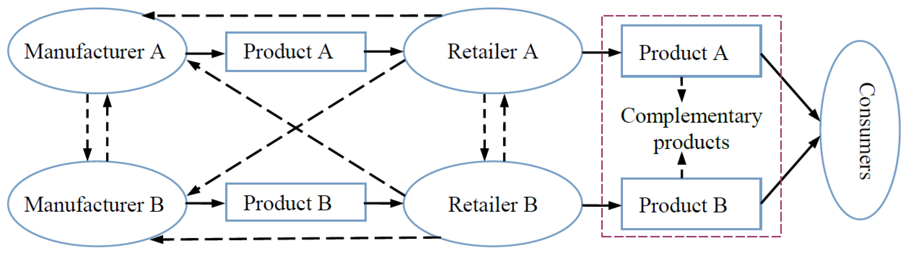
• Assumption 1: Each supply chain consists only of two players, i.e., a manufacturer and a retailer, as shown in Figure 1.
• Assumption 2: All players, lender, manufacturer and retailer, are all rational.
• Assumption 3: Manufacturers cannot afford all their desired production costs only with their initial capitals. Similarly, retailers’ initial capitals cannot fully cover their desired purchasing costs. Only if manufacturers and retailers have cash constraint problems, they will make their effort to get more cash. One of the best choices for manufacturers and retailers is to get some financing loans.
• Assumption 4: Lending rates remained unchanged. That is, the lending rate does not depend on financing amount, manufactures and retailers can get the loan with the same rate.
• Assumption 5: There is no defective product.
• Assumption 6: In dual supply chains, manufacturers are dominant, and retailers’ initial capitals are near zero. The probability for manufacturers and retailers to get loan by themselves is less than 1, but the probability for retailers is less than manufactures’.

2.2. Notation

For the sake of convenience, the following notations with units in

Table 1. Notation list.

Notation	Description	Unit
$a_{m1}$, $a_{m2}$	Initial capitals of MA and MB, respectively.	Million dollar
$a_{r1}$, $a_{r2}$	Initial capitals of RA and RB, respectively.	Million dollar
$x_{m1}$, $x_{m2}$	Financing amounts of MA and MB, respectively.	Million dollar
$x_{r1}$, $x_{r2}$	Financing amounts of RA and RB, respectively.	Million dollar
$Q_1$, $Q_2$	Production quantities of MA and MB, respectively.	Standard quantity unit(SQU)
$q_1$, $q_2$	Order quantities of RA and RB, respectively.	SQU
$c_1$, $c_2$	Unit production costs of products A and B, respectively.	Million dollar/SQU
$c_A$, $c_B$	Salvage values of unsold products A and B, respectively.	Million dollar
$p_a$, $p_b$	Retailers’ purchase prices of the products A and B, respectively.	Million dollar/SQU
$p_1$, $p_2$	Unit sales prices of the products A and B, respectively.	Million dollar/SQU
$r$	lending rates	Percentage/year
$r^{*}$	deposit rates	Percentage/year
${\alpha }_i$, ${\beta }_i$	probability for manufacturers and retailers to get loan by themselves, respectively	Null

are used throughout this paper.

3. A Financing Model of a Single Supply Chain

In this subsection, inspired by Raghavan and Mishra [66], two kind of financing decisions will be proposed for one of dual supply chains with complementary products. One is running on an autonomous track with asymmetric information, the other is running with joint decisions. The former is a traditional financing model with a debtor and its lender. The latter is a joint financing model with all financing enterprises of the supply chain and their lenders. By means of the symmetry between SCA and SCB, one can directly know SCB well from the following studies about SCA.

3.1. Independent Financing Decisions

As a traditional financing model with MA and RA, their independent financing decisions are running in such a scenario, where the information about the cash constraint is asymmetrical for MA and RA.

3.1.1. Independent Financing Decisions of MA

At the beginning of the product period, a manufacturer predicts its retailer’s order quantities by assuming its retailer and the members of its complementary product chain have enough cash holding to pay for their decisions.

RA and RB make their decisions on order quantities and selling prices so as to get their optimal profits. One can define the following MDA and MDB:

$$D_1=d_1-{\lambda }_1{p}_1-{\eta }_1{p}_2,$$

(1)

$$D_2=d_2-{\lambda }_2{p}_2-{\eta }_2{p}_1,$$

(2)

where ${\lambda }_i>{\eta }_i$, and ${\lambda }_i$ represents a self-price sensitivity coefficient, and ${\eta }_i$ represents a cross-price sensitivity coefficient.

One can denote the following profits of RA and RB:

$$E\left({\pi }_{r1}\right)=p_1{q}_1-p_a{q}_1\left(1+r^{*}{T}_r\right),$$

(3)

$$E\left({\pi }_{r2}\right)=p_2{q}_2-p_b{q}_2\left(1+r^{*}{T}_r\right).$$

(4)

Let $\frac{\partial E\left({\pi }_{r1}\right)}{\partial p_1}=0$ and $\frac{\partial E\left({\pi }_{r2}\right)}{\partial p_2}=0$, one can get the selling price estimations of RA and RB as follows:

$${\tilde{p}}_1=\phi \left(2{\lambda }_2{d}_1-{\eta }_1{d}_2+{\lambda }_2\left(2{\lambda }_1{p}_a-{\eta }_1{p}_b\right)\left(1+r^{*}{T}_r\right)\right),$$

(5)

$${\tilde{p}}_2=\phi \left(2{\lambda }_1{d}_2-{\eta }_2{d}_1+{\lambda }_1\left(2{\lambda }_2{p}_b-{\eta }_2{p}_a\right)\left(1+r^{*}{T}_r\right)\right),$$

(6)

where $\phi =\frac{1}{4{\lambda }_1{\lambda }_2-{\eta }_1{\eta }_2}$.

Therefore, MA and MB can predict their own retailer’s order quantities as follows:

$${\tilde{q}}_1={\lambda }_1\phi \left(2{\lambda }_2{d}_1-{\eta }_1{d}_2-\left(\left(2{\lambda }_1{\lambda }_2-{\eta }_1{\eta }_2\right)p_a+{\lambda }_2{\eta }_1{p}_b\right)\left(1+r^{*}{T}_r\right)\right),$$

(7)

$${\tilde{q}}_2={\lambda }_2\phi \left(2{\lambda }_1{d}_2-{\eta }_2{d}_1-\left(\left(2{\lambda }_1{\lambda }_2-{\eta }_1{\eta }_2\right)p_b+{\lambda }_1{\eta }_2{p}_a\right)\left(1+r^{*}{T}_r\right)\right).$$

(8)

${\tilde{q}}_1>a_{m1}/c_1$ holds based on Assumptions 2 and 3, that is, MA can get more profits with loan than without it, so MA needs to approach a lender for loan when it makes product decisions. The loan amount can be denoted as

$$x_{m1}=Q_1{c}_1-a_{m1}$$

(9)

Based on the Assumptions 3–6, there are two cases:

(1)

If the lender gives MA a loan, its profit function is

$${\pi }_{m1}=p_a\min \left\{Q_1,q_1\right\}+c_A\max \left\{Q_1-q_1,0\right\}-a_{m1}\left(1+r^{*}{T}_m\right)-x_{m1}\left(1+r{T}_m\right),$$

(10)

where $c_A<c_1$;

(2)

If the lender refuses to give MA a loan, its profit function is

$${\pi }_{m1}=p_a\min \left\{Q_1,q_1\right\}+c_A\max \left\{Q_1-q_1,0\right\}-a_{m1}\left(1+r^{*}{T}_m\right),$$

(11)

where $c_A<c_1$.

Therefore, MA’s expected profit can be given by

$$\begin{array}{cc}{E}_0\left({\pi }_{m1}\right)& ={\alpha }_1\left(p_a\min \left\{Q_1,q_1\right\}+c_A\max \left\{Q_1-q_1,0\right\}-a_m\left(1+r^{*}{T}_m\right)-x_m\left(1+r{T}_m\right)\right)\hfill \\ & +\left(1-{\alpha }_1\right)\left(p_a\min \left\{Q_1,q_1\right\}+c_A\max \left\{Q_1-q_1,0\right\}-a_m\left(1+r^{*}{T}_m\right)\right).\hfill \end{array}$$

(12)

In this function, this term ${\alpha }_1(•)$ represents the profit that MA gets after he gets loans, and $a_{m1}\left(1+r^{*}{T}_m\right)+x_{m1}\left(1+r{T}_m\right)$ is the cost, and $\left(1-{\alpha }_1\right)(•)$ represents the profit that MA gets after he fails to get loans, and $a_m\left(1+r^{*}{T}_m\right)$ is the cost. This function has the same structure to Equation (12).

And the lender’s expected profit function is:

$$\begin{array}{cc}E\left({\pi }_{l1}\right)& ={\alpha }_1\left(\min \left\{x_m\left(1+r{T}_m\right),p_a\min \left\{Q_1,q_1\right\}+c_A\max \left\{Q_1-q_1,0\right\}\right\}-x_m\left(1+r^{*}{T}_m\right)\right)\hfill \\ & +\left(1-{\alpha }_1\right)x_m\left(1+r^{*}{T}_m\right).\hfill \end{array}$$

(13)

3.1.2. Independent financing decisions of RA

Similar to MA’s independent financing decisions, RA will make an order decisions at the beginning of its selling period by predicting the market demand and get $q_1$ units products from MA. When RA makes the prediction about the market demand, it thinks there is no cash contraction with its retailer and the members of its complementary product chain, that is, in this case, $p_2={\tilde{p}}_2$.

Based on the Assumption 3, RA needs the following loan amount from the lender to pay its orders.

$$x_{r1}=q_1{p}_a-a_{r1},$$

(14)

where $q_1$ is equal to its estimation for MDA, which can be obtained by solving the following optimization problem:

$$E\left({\pi }_{r1}\right)=p_1{q}_1-a_{r1}\left(1+r^{*}{T}_r\right)-\left(q_1{p}_a-a_{r1}\right)\left(1+r{T}_r\right).$$

(15)

Let $\frac{\partial E\left({\pi }_{r1}\right)}{\partial p_1}=0$ with $p_2={\tilde{p}}_2$, one can get

$$p_1=\phi \left(2{\lambda }_2{d}_1-{\eta }_1{d}_2-{\eta }_1{\lambda }_2{p}_b\left(1+r^{*}{T}_r\right)-\frac{{\eta }_1{\eta }_2\left(r-r^{*}\right)p_a}{2}+2{\lambda }_1{\lambda }_2{p}_a\left(1+r{T}_r\right)\right).$$

(16)

Therefore, RA can predict MDA as follows:

$${\tilde{D}}_1={\lambda }_1\left(\phi \left(\left(2{\lambda }_2{d}_1-{\eta }_1{d}_2\right)-{\lambda }_2{\eta }_1{p}_b\left(1+r^{*}{T}_r\right)\right)-\frac{p_a\left(\left(1+r{T}_r\right)-\phi {\eta }_1{\eta }_2\left(1+r^{*}{T}_r\right)\right)}{2}\right),$$

(17)

Based on Assumptions 3–6, there are also two cases:

• If RA can get a loan from its lender, its profit function can be determined by:

  $$\begin{array}{cc}{\pi }_{r1}& =p_1\min \left\{Q_1,q_1,D_1\right\}+p_a\max \left\{q_1-Q_1,0\right\}\left(1+r^{*}{T}_r\right)\hfill \\ & +c_A\max \left\{\min \left\{Q_1,q_1\right\}-D_1,0\right\}-a_{r1}\left(1+r^{*}{T}_r\right)-x_{r1}\left(1+r{T}_r\right)\hfill \end{array};$$

  (18)
• If RA failed to get a loan, its profit function can be determined by:

  $${\pi }_{r1}=p_1{q}_1-a_{r1}\left(1+r^{*}{T}_r\right).$$

  (19)

Therefore, RA can obtain its expected profit as:

$$\begin{array}{cc}{E}_0\left({\pi }_{r1}\right)& ={\beta }_1\left(\begin{array}{c}{p}_1\min \left\{Q_1,q_1,D_1\right\}+p_a\max \left\{q_1-Q_1,0\right\}\left(1+r^{*}{T}_r\right)\hfill \\ +c_A\max \left\{\min \left\{q_1,Q_1\right\}-D_1,0\right\}-a_{r1}\left(1+r^{*}\right)T_r-x_{r1}\left(1+r\right)T_r\hfill \end{array}\right)\hfill \\ & +\left(1-{\beta }_1\right)\left(p_1{q}_1-a_{r1}\left(1+r^{*}{T}_r\right)\right).\hfill \end{array}$$

(20)

And the lender can get its expected profit as:

$$\begin{array}{cc}E\left({\pi }_{l1}\right)& ={\beta }_1\left(\min \left(\begin{array}{l}{x}_{r1}\left(1+r{T}_r\right),p_1\min \left\{Q_1,q_1,D_1\right\}\\ +p_a\max \left\{q_1-Q_1,0\right\}\left(1+r^{*}{T}_r\right)\\ +c_A\max \left\{\min \left\{q_1,Q_1\right\}-D_1,0\right\}\end{array}\right)-x_{r1}\left(1+r^{*}{T}_r\right)\right)\hfill \\ & +\left(1-{\beta }_1\right)x_{r1}\left(1+r^{*}{T}_r\right)\hfill \end{array}.$$

(21)

3.1.3. Analyses on Independent Financing Decisions

In independent financing decisions, the information between MA and RA is asymmetric. MA makes its production decisions by assuming RA has enough cash holding to pay its orders. Similarly, RA makes its order decisions under the assumption that MA’s production capacity is sufficient for its orders. However, the capital constraint is the biggest obstacle to increasing profits of both MA and RA, which turns them into striving to get a loan from lenders.

Case 1. 

A lender would like to provide loans to both MA and RA.

As mentioned above, $Q_1={\tilde{q}}_1$ and $q_1={\tilde{D}}_1$ satisfy,

$$Q_1-q_1={\lambda }_1{p}_a\left(\frac{\left(\left(1+r{T}_r\right)-\phi {\eta }_1{\eta }_2\left(1+r^{*}{T}_r\right)\right)}{2}-\phi \left(2{\lambda }_1{\lambda }_2-{\eta }_1{\eta }_2\right)\left(1+r^{*}{T}_r\right)\right)>0.$$

i.e., $Q_1>q_1$ which means MA is not sold out of its products though it completely fulfills RA’s orders. Obviously MA’s overproduction will neutralize a part of its profits. In order to solve this problem, MA will make efforts to get RA’s demand more accurately. Therefore, one can get the following profits of MA and RA:

$${\pi }_{m1}^1=p_a{\tilde{D}}_1+c_A\left({\tilde{q}}_1-{\tilde{D}}_1\right)-a_{m1}\left(1+r^{*}{T}_m\right)-x_{m1}\left(1+r{T}_m\right),$$

(22)

$${\pi }_{r1}^1=p_1\min \left\{{\tilde{D}}_1,D_1\right\}+c_A\max \left\{{\tilde{D}}_1-D_1,0\right\}-a_{r1}\left(1+r^{*}{T}_r\right)-x_{r1}\left(1+r{T}_r\right).$$

(23)

Case 2. 

The lender provides a loan only to MA but not to RA.

MA gets the loan and makes all the cash available to its production, i.e., $Q_1={\tilde{q}}_1$, but RA has only the initial capitals $a_{r1}$ available to make its orders, i.e., $q_1=\frac{a_{r1}}{p_a}$. Obviously, $Q_1>q_1$ holds and means MA is not able to fulfill RA’s orders. The profits of MA and RA are

$${\pi }_{m1}^2=p_a\frac{a_{r1}}{p_a}+c_A\left({\tilde{q}}_1-\frac{a_{r1}}{p_a}\right)-a_{m1}\left(1+r^{*}{T}_m\right)-x_{m1}\left(1+r{T}_m\right),$$

(24)

$${\pi }_{r1}^2=p_1\frac{a_{r1}}{p_a}-a_{r1}\left(1+r^{*}{T}_r\right).$$

(25)

As a result, MA will get less profits and even go bankrupt if

$$Q_1={\tilde{q}}_1>\frac{a_{r1}-c_A\frac{a_{r1}}{p_a}+x_{m1}\left(1+r{T}_m\right)}{c_1\left(1+r{T}_m\right)-c_A}.$$

Therefore, MA’s profit will arise with RA’s order quantity $q_1$ increasing. It is a smart choice for MA to help RA to get more cash to make more order.

Case 3. 

The lender provides a loan only to RA but not to MA.

MA only has the initial capitals $a_{m1}$ for its production, i.e., $Q_1=\frac{a_{m1}}{c_1}$, but RA’s demand is $q_1={\tilde{D}}_1$. Obviously, $Q_1<q_1$ holds, which means MA is not able to fulfill RA’s orders. The profits of MA and RA can be represented as follows:

$${\pi }_{m1}^3=p_a\frac{a_{m1}}{c_1}-a_{m1}\left(1+r^{*}{T}_m\right),$$

(26)

$$\begin{array}{cc}{\pi }_{r1}^3& =p_1\frac{a_{m1}}{c_1}+p_a\left({\tilde{D}}_1-\frac{a_{m1}}{c_1}\right)\left(1+r^{*}{T}_r\right)+c_A\max \left\{\frac{a_{m1}}{c_1}-D_1,0\right\}\hfill \\ & -a_{r1}\left(1+r^{*}{T}_r\right)-x_{r1}\left(1+r{T}_r\right)\hfill \end{array}.$$

(27)

Case 4. 

The lender refuses all loan applications from both MA and RA.

MA’s production and RA’s order are only supported by their initial capitals, respectively, i.e., $Q_1=\frac{a_{m1}}{c_1}$, $q_1=\frac{a_{r1}}{p_a}$. Obviously, $Q_1>q_1$ holds based on Assumption 6, which means MA produces more products than RA’s orders. The profits of MA and RA can be written as follows:

$${\pi }_{m1}^4=p_a\frac{a_{r1}}{p_a}+c_A\left(\frac{a_{m1}}{c_1}-\frac{a_{r1}}{p_a}\right)-a_{m1}\left(1+r^{*}{T}_m\right),$$

(28)

$${\pi }_{r1}^4=p_1\frac{a_{r1}}{p_a}-a_{r1}\left(1+r^{*}{T}_r\right).$$

(29)

In any case, $Q_1\ne q_1$ holds, i.e., MA’s product quantity and RA’s order can not reach equilibrium. Therefore, not only would MA like to make a joint financing decision with the retailer in order to understand RA’s demand more accurately, but also would the retailer like to do the same joint financing decision with MA to get a loan more successfully.

In addition, we can get the following expected profits of MA and RA with their independent financing decisions:

$$E_1\left({\pi }_{m1}\right)={\alpha }_1{\beta }_1{\pi }_{m1}^1+{\alpha }_1\left(1-{\beta }_1\right){\pi }_{m1}^2+{\beta }_1\left(1-{\alpha }_1\right){\pi }_{m1}^3+\left(1-{\alpha }_1\right)\left(1-{\beta }_1\right){\pi }_{m1}^4,$$

(30)

$$E_1\left({\pi }_{r1}\right)={\alpha }_1{\beta }_1{\pi }_{r1}^1+{\alpha }_1\left(1-{\beta }_1\right){\pi }_{r1}^2+{\beta }_1\left(1-{\alpha }_1\right){\pi }_{r1}^3+\left(1-{\alpha }_1\right)\left(1-{\beta }_1\right){\pi }_{r1}^4.$$

(31)

3.2. Joint Financing Decisions of SCA

Unlike the case of the independent decision mentioned above, the information about the cash constraint is symmetrical for MA and RA in such a scenario of the joint financing decision.

3.2.1. A Joint Financing Model

One can get their financing amounts by finding quantity equilibrium between their production and order which can be regarded as a Stackelberg game. In this game, MA is the leader and RA is the follower and $Q_1=q_1={\widehat{q}}_1={\tilde{D}}_1$ holds at the equilibrium. Therefore, the loan amounts of MA and RA can be written as follows:

$${\widehat{x}}_{m1}={\widehat{q}}_1{c}_1-a_{m1},$$

(32)

$${\widehat{x}}_{r1}={\widehat{q}}_1{p}_a-a_{r1},$$

(33)

The joint financing contract in the supply chain is open to the lender. With the consideration of risk, the lender prefers to give a loan to the supply chain alliance rather than one of members of SCA. However, there still are two cases: loan or not. $\alpha$ can be employed to denote the loan probability for SCA, where $\alpha >{\alpha }_1>{\beta }_1$, and $\beta$ can be used to denote the loan probability for SCB, where $\beta >{\alpha }_2>{\beta }_2$.

• If the lender provides a loan to SCA, profit functions of MA and RA are

  $$\begin{array}{cc}{\widehat{\pi }}_{m1}^1& =\left(p_a{\widehat{q}}_1-{\widehat{x}}_{m1}\left(1+r{T}_m\right)\right)\left(1+r^{*}{T}_r\right)-a_{m1}\left(1+r^{*}{T}_m\right)\hfill \\ & -\max \left\{{\widehat{x}}_{r1}\left(1+r{T}_r\right)-{\widehat{p}}_1\min \left\{{\widehat{q}}_1,D_1\right\}+c_A\max \left\{{\widehat{q}}_1-D_1,0\right\},0\right\}\hfill \end{array},$$

  (34)

  $${\widehat{\pi }}_{r1}^1={\widehat{p}}_1\min \left\{{\widehat{q}}_1,D_1\right\}+c_A\max \left\{{\widehat{q}}_1-D_1,0\right\}-a_{r1}\left(1+r^{*}{T}_r\right)-{\widehat{x}}_{r1}\left(1+r{T}_r\right),$$

  (35)

  where ${\widehat{p}}_1=p_1$,

In fact, it is more possible for RA to default the joint financing contract than for MA because MA has transferred the market risk into RA by the joint financing contract. Since MA and RA are a joint financing alliance of a supply chain, they all should be jointly and severally liable to the lender. Therefore, MA has to repay RA’s loan if RA fails to pay it, which is shown the last term of Equation (34).

• If the lender refused their joint financing contract, the quantity equilibrium of MA's production and RA’s order satisfies $Q_1=q_1=\frac{a_{r1}}{p_a}<\frac{a_{m1}}{c_1}$. Therefore, their profit functions are written as

  $${\widehat{\pi }}_{m1}^2=\left(p_a-c_1\left(1+r^{*}{T}_m\right)\right)\frac{a_{r1}}{p_a},$$

  (36)

  $${\widehat{\pi }}_{r1}^2=p_1\frac{a_{r1}}{p_a}-a_{r1}\left(1+r^{*}{T}_r\right),$$

  (37)

Therefore, the expected profit functions of MA and RA can be obtained as follows

$$E\left({\widehat{\pi }}_{m1}\right)=\alpha {\widehat{\pi }}_{m1}^1+\left(1-\alpha \right){\widehat{\pi }}_{m1}^2,$$

(38)

$$E\left({\widehat{\pi }}_{r1}\right)=\alpha {\widehat{\pi }}_{r1}^1+\left(1-\alpha \right){\widehat{\pi }}_{r1}^2.$$

(39)

In addition, the lender’s expected profit function can be represented as follows.

$$E\left({\widehat{\pi }}_{lA}\right)=\alpha \left({\widehat{\pi }}_{lm}+{\widehat{\pi }}_{lr}\right),$$

(40)

where

$${\widehat{\pi }}_{lm}={\widehat{x}}_{m1}\left(1+r{T}_m\right)-{\widehat{x}}_{m1}\left(1+r^{*}{T}_m\right),$$

$${\widehat{\pi }}_{lr}=\min \left\{\begin{array}{l}{\widehat{x}}_{r1}\left(1+r{T}_r\right),{\widehat{p}}_1\min \left\{{\widehat{q}}_1,D_1\right\}+c_A\max \left\{{\widehat{q}}_1-D_1,0\right\}\\ +\left(p_a{\widehat{q}}_1-{\widehat{x}}_{m1}\left(1+r{T}_m\right)\right)\left(1+r^{*}{T}_r\right)\end{array}\right\}-{\widehat{x}}_{r1}\left(1+r^{*}{T}_r\right),$$

3.2.2. Analyses on Joint Financing Decisions

When SCA makes its joint financing decisions, it assumes SCB has enough cash holding to make its decisions though the assumption is wrong. If SCA’s joint financing is successful, there are two cases as follows.

Case 1. 

MB and RB fail in their joint financing.

Similar to SCA, MB’s output is equal to RB’ sales, i.e., $Q_2=q_2=a_{r2}/p_b$, so one can get the following MDA.

$${\widehat{D}}_1^1=d_1-{\lambda }_1{p}_1-\frac{{\eta }_1}{{\lambda }_2}\left(d_2-\frac{a_{r2}}{p_b}-{\eta }_2{\tilde{p}}_1\right).$$

(41)

Obviously, ${\tilde{D}}_1-{\widehat{D}}_1^1>0$ holds, so profit functions of MA and RA can be written by

$$\begin{array}{cc}{\widehat{\pi }}_{m1}^3& =\left(p_a{\widehat{q}}_1-{\widehat{x}}_{m1}\left(1+r{T}_m\right)\right)\left(1+r^{*}{T}_r\right)-a_{m1}\left(1+r^{*}{T}_m\right)\hfill \\ & -\max \left\{{\widehat{x}}_{r1}\left(1+r{T}_r\right)-{\widehat{p}}_1{\widehat{D}}_1^1+c_A\left({\widehat{q}}_1-{\widehat{D}}_1^1\right)\right\}\hfill \end{array},$$

(42)

$${\widehat{\pi }}_{r1}^3={\widehat{p}}_1{\widehat{D}}_1^1+c_A\left({\widehat{q}}_1-{\widehat{D}}_1^1\right)-a_{r1}\left(1+r^{*}{T}_r\right)-{\widehat{x}}_{r1}\left(1+r{T}_r\right).$$

(43)

Case 2. 

MB and RB are successful in their joint financing.

According to the symmetry between SCA and SCB, one can get $p_2>{\tilde{p}}_2$ from $p_1>{\tilde{p}}_1$, so MDA satisfies ${\widehat{D}}_1^2<{\tilde{D}}_1$ and ${\widehat{D}}_1^2=d_1-{\lambda }_1{\widehat{p}}_1-{\eta }_1{p}_2$. The profit functions of MA and RA can be rewritten as follows.

$$\begin{array}{cc}{\widehat{\pi }}_{m1}^4& =p_a{\widehat{q}}_1-{\widehat{x}}_{m1}\left(1+r{T}_m\right)\left(1+r^{*}{T}_r\right)-a_{m1}\left(1+r^{*}{T}_m\right)\hfill \\ & -\max \left\{\begin{array}{cc}{\widehat{x}}_{r1}\left(1+r{T}_r\right)-{\widehat{p}}_1{\widehat{D}}_1^2+c_A\left({\widehat{q}}_{\mathbf{1}}-{\widehat{D}}_1^2\right),& 0\end{array}\right\}\hfill \end{array},$$

(44)

$${\widehat{\pi }}_{r1}^4={\widehat{p}}_1{\widehat{D}}_1^2+c_A\left({\widehat{q}}_1-{\widehat{D}}_1^2\right)-a_{r1}\left(1+r^{*}{T}_r\right)-{\widehat{x}}_{r1}\left(1+r{T}_r\right).$$

(45)

Therefore, the expected profits of MA and RA are expressed as follows

$$E\left({\widehat{\pi }}_{m1}\right)=\alpha \left(1-\beta \right){\widehat{\pi }}_{m1}^3+\alpha \beta {\widehat{\pi }}_{m1}^4+\left(1-\alpha \right){\widehat{\pi }}_{m1}^2,$$

(46)

$$E\left({\widehat{\pi }}_{r1}\right)=\alpha \left(1-\beta \right){\widehat{\pi }}_{r1}^3+\alpha \beta {\widehat{\pi }}_{r1}^4+\left(1-\alpha \right){\widehat{\pi }}_{r1}^2.$$

(47)

In the case of joint financings, both MA and MB can balance supply and demand within SCA and SCB, respectively. However, there exit some deviations for SCA and SCB to predict the demands of their complementary products. Therefore, it is a smart choice for SCA and SCB to make a joint financing decision with each other to optimize their productions.

3.3. Comparisons of Independent Decisions and Joint Financing Decisions of SCA

When both MA and RA make an independent financing or a joint financing decision, they assume the product B can be provided without any constraints. The following comparisons can be made as:

• For MA, One can get its expected profit with the independent financing decision as shown in Equation (30) and its expected profit with the joint financing decision as follows.

  $$\begin{array}{cc}E\left({\widehat{\pi }}_{m1}\right)& =\alpha \left(p_a{\widehat{q}}_1-{\widehat{x}}_{m1}\left(1+r{T}_m\right)-a_{m1}\left(1+r^{*}{T}_m\right)\right)+\hfill \\ & \left(1-\alpha \right)\left(\left(p_a-c_1\left(1+r^{*}{T}_m\right)\right)\frac{a_{r1}}{p_a}\right)\hfill \end{array}$$

  (48)
  So their difference is

  $$\Delta E\left({\pi }_{m1}\right)=E\left({\widehat{\pi }}_{m1}\right)-E_0\left({\pi }_{m1}\right)>0$$

  which says the joint financing decision is better than the independent financing decision for MA.
• For RA, it is easy to get its expected profits with the independent decisions and joint financing decisions, respectively, as follows:

  $$\begin{array}{cc}E\left({\pi }_{r1}\right)& ={\alpha }_1{\beta }_1\left(p_1{\tilde{D}}_1-a_{r1}\left(1+r^{*}{T}_r\right)-x_{r1}\left(1+r{T}_r\right)\right)+{\alpha }_1\left(1-{\beta }_1\right)\left(p_1\frac{a_{r1}}{p_a}-a_{r1}\left(1+r^{*}{T}_r\right)\right)\hfill \\ & +{\beta }_1\left(1-{\alpha }_1\right)\left(p_1\frac{a_{m1}}{c_1}+p_a\left({\tilde{D}}_1-\frac{a_{m1}}{c_1}\right)\left(1+r^{*}{T}_r\right)-a_{r1}\left(1+r^{*}{T}_r\right)-x_{r1}\left(1+r{T}_r\right)\right)\hfill \\ & +\left(1-{\alpha }_1\right)\left(1-{\beta }_1\right)\left(p_1\frac{a_{r1}}{p_a}-a_{r1}\left(1+r^{*}{T}_r\right)\right),\hfill \end{array}$$

  $$E\left({\widehat{\pi }}_{r1}\right)=\alpha \left({\widehat{p}}_1{\widehat{q}}_1-a_{r1}\left(1+r^{*}{T}_r\right)-{\widehat{x}}_{r1}\left(1+r{T}_r\right)\right)+\left(1-\alpha \right)\left(p_1\frac{a_{r1}}{p_a}-a_{r1}\left(1+r^{*}{T}_r\right)\right)$$

  Therefore, their difference is

  $$\Delta E\left({\pi }_{r1}\right)=E\left({\widehat{\pi }}_{r1}\right)-E\left({\pi }_{r1}\right)>0$$

  which shows RB is rational to make a joint financing decision rather than an independent financing decision.

To sum up, if all enterprises in the supply chain faced capital constraints, it is the best way for them not to make an independent financing decision but to make a joint financing decision.

4. A Joint Financing Model of SCA and SCB

4.1. A Joint Financing Model of SCA and SCB

If there exists a joint financing of SCA and SCB, it is easy for SCA and SCB to know initial capitals and loan demands of their counterparts. As a result, they both can grasp their market demands more accurately than before.

By solving the following optimization problem, one can get loan amounts of MA, RA, MB and RB, respectively.

$$\{\begin{array}{l}E\left({\pi }_{r1}\right)=p_1{q}_1-a_{r1}\left(1+r^{*}{T}_r\right)-\left(q_1{p}_a-a_{r1}\right)\left(1+r{T}_r\right),\\ E\left({\pi }_{r2}\right)=p_2{q}_2-a_{r2}\left(1+r^{*}{T}_r\right)-\left(q_2{p}_b-a_{r2}\right)\left(1+r{T}_r\right).\end{array}$$

(49)

in which $p_1$, $q_1$, $p_2$, and $q_2$ satisfy the following functions:

$$\{\begin{array}{l}{q}_1=d_1-{\lambda }_1{p}_1-{\eta }_1{p}_2,\\ q_2=d_2-{\lambda }_2{p}_2-{\eta }_2{p}_1.\end{array}$$

(50)

From Equations (49) and (50), one can get the following expressions:

$$\{\begin{array}{l}{p}_1^{*}=\phi \left(2{\lambda }_2{d}_1-{\eta }_1{d}_2+2{\lambda }_1{\lambda }_2{p}_a\left(1+r{T}_r\right)-{\eta }_1{\lambda }_2{p}_b\left(1+r{T}_r\right)\right),\\ p_2^{*}=\phi \left(2{\lambda }_1{d}_2-{\eta }_2{d}_1+2{\lambda }_1{\lambda }_2{p}_b\left(1+r{T}_r\right)-{\eta }_2{\lambda }_1{p}_a\left(1+r{T}_r\right)\right).\end{array}$$

(51)

and the following equations hold.

$$\{\begin{array}{l}{q}_1^{*}=d_1-{\lambda }_1{p}_1^{*}-{\eta }_1{p}_2^{*},\\ q_2^{*}=d_2-{\lambda }_2{p}_2^{*}-{\eta }_2{p}_1^{*}.\end{array}$$

(52)

From Equations (51) and (52), one can get the following loan amounts of MA, RA, MB and RB, respectively.

$$x_{m1}^{*}=q_1^{*}{c}_1-a_{m1},$$

(53)

$$x_{r1}^{*}=q_1^{*}{p}_a-a_{r1},$$

(54)

$$x_{m2}^{*}=q_2^{*}{c}_2-a_{m2},$$

(55)

$$x_{r2}^{*}=q_2^{*}{p}_b-a_{r2}.$$

(56)

From Equations (51)–(56), it is easy to obtain the following profits of MA, RA, MB and RB, respectively.

$${\pi }_{m1}^{*}=p_a{q}_1^{*}-\left(a_{m1}\left(1+r^{*}{T}_m\right)+x_{m1}^{*}\left(1+r{T}_m\right)\right),$$

(57)

$${\pi }_{r1}^{*}=p_1^{*}{q}_1^{*}-\left(a_{r1}\left(1+r^{*}{T}_m\right)+x_{r1}^{*}\left(1+r{T}_m\right)\right),$$

(58)

$${\pi }_{m2}^{*}=p_b{q}_2^{*}-\left(a_{m2}\left(1+r^{*}{T}_m\right)+x_{m2}^{*}\left(1+r{T}_m\right)\right),$$

(59)

$${\pi }_{r2}^{*}=p_2^{*}{q}_2^{*}-\left(a_{r2}\left(1+r^{*}{T}_m\right)+x_{r2}^{*}\left(1+r{T}_m\right)\right).$$

(60)

Therefore, the lender’s profit from SCA and SCB is:

$${\pi }_l=\left(x_{m1}^{*}+x_{m2}^{*}\right)\left(1+r{T}_m\right)+\left(x_{r1}^{*}+x_{r2}^{*}\right)\left(1+r{T}_r\right).$$

(61)

4.2. Comparison of Different Financing Decisions of SCA and SCB

Similar to section 3.3, when the single SCA or both SCA and SCB make joint financing decisions, one can get their following profit differences of MA and RA from Equations (46), (47), (53) and (54) as follows.

$$\Delta E\left({\pi }_{m1}\right)=E\left({\pi }_{m1}^{*}\right)-E_1\left({\widehat{\pi }}_{m1}\right)>0,$$

(62)

$$\Delta E\left({\pi }_{r1}\right)=E\left({\pi }_{r1}^{*}\right)-E_1\left({\widehat{\pi }}_{r1}\right)>0,$$

(63)

from which, one can find MA’s profit with the join financing decision of the single SCA is less than that of both SCA and SCB, so the latter is a smart choice for it. At the same time, from the perspective of the RA, joint financing decision of SCA and SCB is a better choice for it than join financing of business in SCA.

5. Numerical Study

As mentioned above, there are three kinds of financing decisions of SCA and SCB: the independent decisions and joint financing decisions of a single supply chain, the joint financing decision of SCA and SCB. In order to make an intuitive understanding about these models, especially the effect of initial capital and products degree of complementarity to the choice of financing decisions, we show some numerical studies of these models in that section. Following show some numerical results of these models as fix $r=0.1$, $r^{*}=0.06$, $T_m=T_r=1$, $d_1=300$, $d_2=150$, $p_a=100$, $p_b=60$, $c_1=25$, $c_2=20$, $c_A=20$, $c_B=15$, ${\lambda }_1=0.7$, ${\lambda }_2=0.8$, ${\alpha }_1=0.6$, ${\beta }_1=0.4$, $\alpha =0.8$, $\beta =0.7$, $a_{r2}=120$.

5.1. Simulations for the Financing Model of a Single Supply Chain

Figure 2a,b show that both MA and RA can get more profits with joint financing decisions than those with independent financing decisions when $a_{m1}$ and $a_{r1}$ vary. What is more, one can find profits of MA and RA increase with $a_{m1}$ and $a_{r1}$ when they are with low initial capitals.

Figure 3a,b show how cross-price sensitivity coefficients have impact on profits of MA and RA with independent financing decisions and joint financing decisions, respectively. Obviously, both MA and RA can get more profits with joint financing decisions than those with independent financing decisions when ${\eta }_1$ and ${\eta }_2$ vary with fixed $a_{m1}=150$ and $a_{r1}=100$. Profits of MA and RA increase with ${\eta }_1$ but decrease with ${\eta }_2$.

Figure 2 and Figure 3 show the joint financing decision is a better choice for MA and RA than the independent financing decisions in SCA.

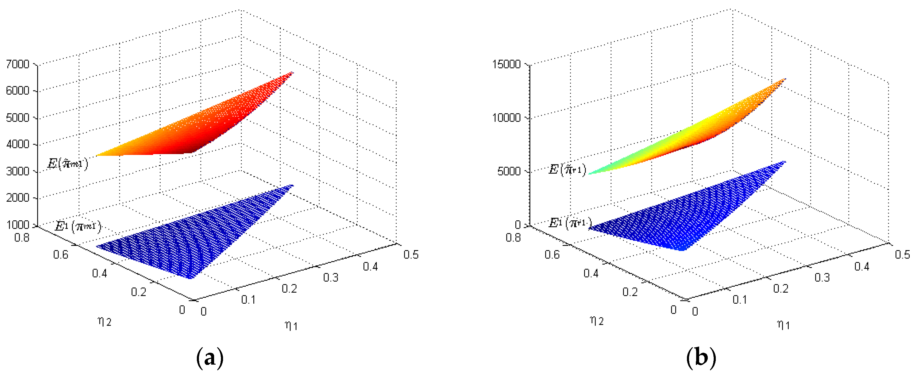
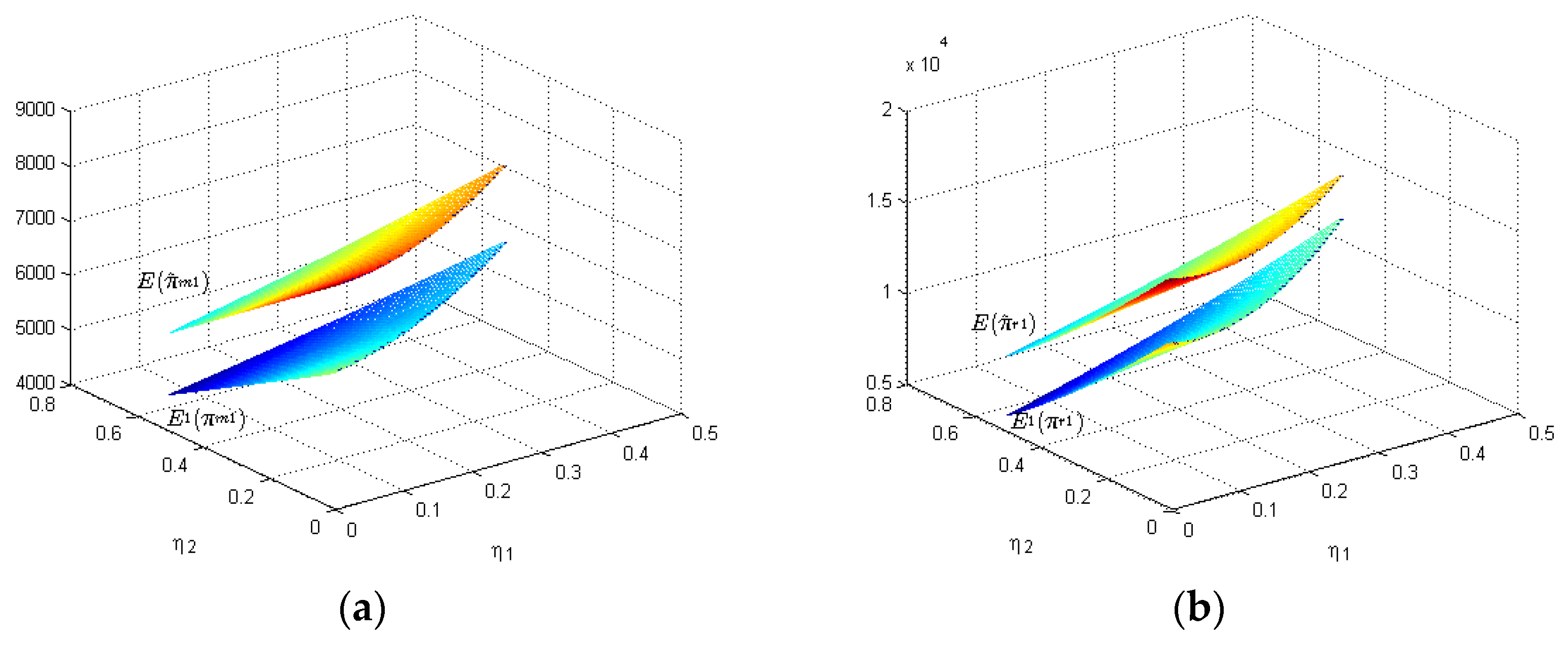
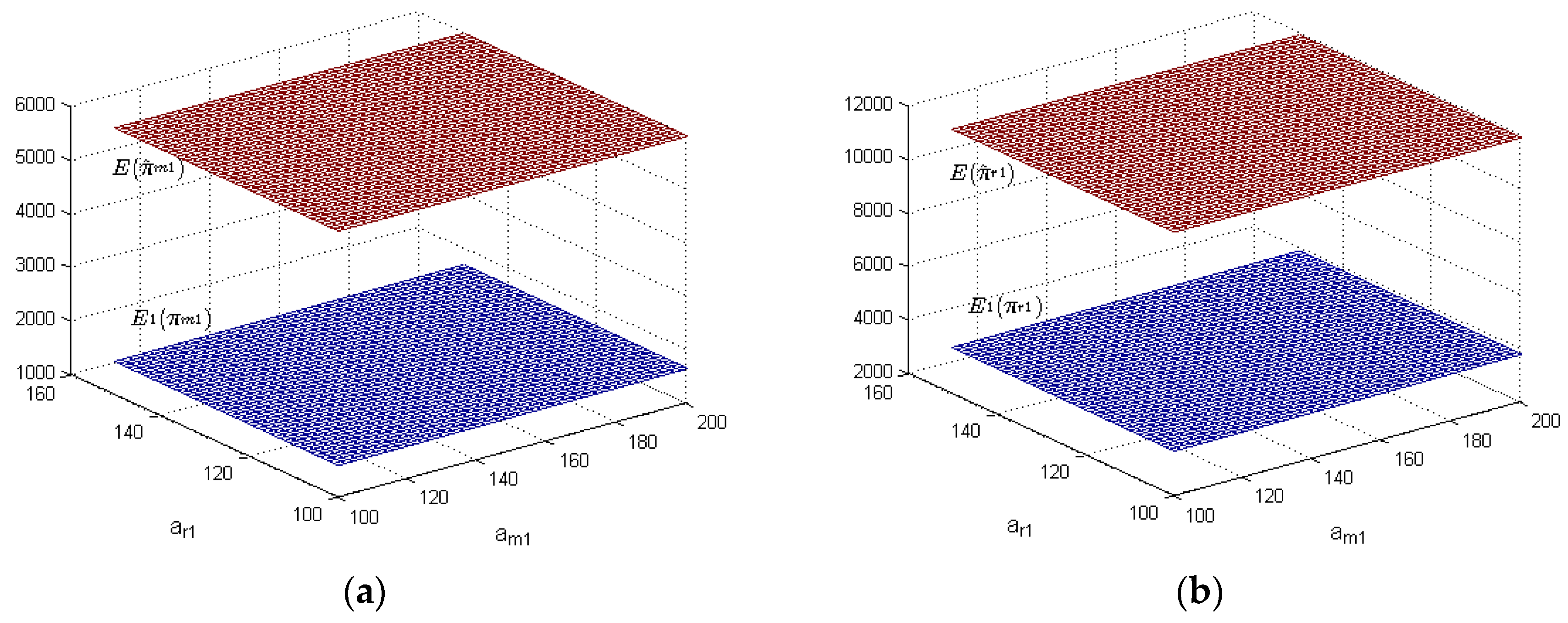
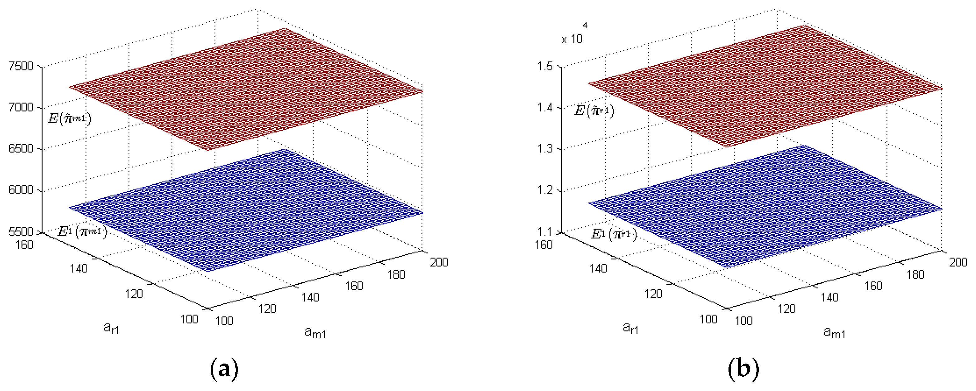
5.2. Simulations for the Joint Financing Model of SCA and SCB

Considering the symmetry between SCA and SCB, one can only illustrate profits variation of MA and RA as shown in the following Figure 4 and Figure 5.

Similar to the single SCA in Figure 2, Figure 4a,b also show that both MA and RA can get more profits with joint financing decisions than those with independent financing decisions. MA’s profits increase with $a_{m1}$ and $a_{r1}$, and RA’s profits increase with $a_{r1}$ but have no relationship with $a_{m1}$.

Figure 5a,b show two facts as follows:

• Both MA and RA can obtain more profits with joint financing decisions than those with independent financing decisions.
• Bigger are cross-price sensitivity coefficients, higher are profits of MA and RA with independent financing decisions and joint financing decisions.

Similar to Figure 2 and Figure 3, Figure 4 and Figure 5 show the joint financing decision is a better choice for MA and RA than the independent financing decisions in SCA and SCB.

In a word, Figure 2, Figure 3, Figure 4 and Figure 5 show the joint financing decision in SCA and SCB is the best for MA and RA among all financing decisions mentioned above.

6. Conclusions

In this paper, we study three kinds of financing decisions of supply chains with complementary products, and find that the best one is the joint financing decision of the two supply chains. Note that our results are based on low initial capitals of members of supply chains. What is more, bigger cross-price sensitivity coefficients can bring participants higher motivation to make joint financing decisions and make them gain higher profits. Therefore, this study has a reference value for supply chain management and financing decisions, especially for SMEs to deal with the cash constrains problem. Furthermore, the cooperative competition is found in joint financing decisions of intra-/inter-supply chains.

Certainly, as a complex supply chain financing system, it is difficult for us to completely analyze it, so there still exist some limitations, such as the absence of other market participants’ effect on market demands, the simplified structures of supply chains. Thus, we may further consider financing decisions of a supply chain network, joint financing decisions of supply chains in specific situations and special occasions, and so on.

References

1. Liu, X.; Zhou, L.; Wu, Y.-C.J. Supply Chain Finance in China: Business Innovation and Theory Development. Sustainability 2015, 7, 14689–14709. [Google Scholar] [CrossRef]
2. Ni, J.Z.; Flynn, B.B.; Jacobs, F.R. Impact of product recall announcements on retailers׳ financial value. Int. J. Prod. Econ. 2014, 153, 309–322. [Google Scholar] [CrossRef]
3. Wuttke, D.A.; Blome, C.; Henke, M. Focusing the financial flow of supply chains: An empirical investigation of financial supply chain management. Int. J. Prod. Econ. 2013, 145, 773–789. [Google Scholar] [CrossRef]
4. Wang, Y.; Zhang, Y. Remanufacturer’s production strategy with capital constraint and differentiated demand. J. Intell. Manuf. 2014, 11, 1–14. [Google Scholar] [CrossRef]
5. Sarkar, B.; Sana, S.; Chaudhuri, K. Optimal reliability, production lotsize and safety stockn economic manufacturing quantity model. Int. J. Manag. Sci. Eng. Manag. 2010, 5, 192–202. [Google Scholar]
6. Sarkar, B.; Mandal, B.; Sarkar, S. Quality improvement and backorder price discount under controllable lead time in an inventory model. J. Manuf. Syst. 2014, 35, 26–36. [Google Scholar] [CrossRef]
7. Sarkar, B.; Majumder, A. Integrated vendor-buyer supply chain model with vendor’s setup cost reduction. Appl. Math. Comput. 2013, 224, 362–371. [Google Scholar] [CrossRef]
8. Sarkar, B.; Gupta, H.; Chaudhuri, K.; Goyald, S.K. An integrated inventory model with variable lead time, defective units and delay in payments. Appl. Math. Comput. 2014, 237, 650–658. [Google Scholar] [CrossRef]
9. Cárdenas-Barrón, L.; Sarkar, B.; Treviño-Garza, G. Easy and improved algorithms to joint determination of the replenishment lot size and number of shipments for an EPQ model with rework. Appl. Math. Comput. 2013, 18, 132–138. [Google Scholar]
10. Sarkar, B.; Saren, S. An inventory model with trade-credit policy and variable deterioration for fixed lifetime products. Ann. Oper. Res. 2014, 229, 677–702. [Google Scholar] [CrossRef]
11. Sarkar, B. A production-inventory model with probabilistic deterioration in two-echelon supply chain management. Appl. Math. Model. 2013, 37, 3138–3151. [Google Scholar] [CrossRef]
12. Chong, T.; Lu, L.; Ongena, S. Does Banking Competition Alleviate or Worsen Credit Constraints Faced by Small- and Medium-Sized Enterprises? Evidence from China. J. Bank. Financ. 2013, 37, 3412–3424. [Google Scholar] [CrossRef]
13. Dong, Y.; Men, C. SME Financing in Emerging Markets: Firm Characteristics, Banking Structure and Institutions. Emerg. Mark. Financ. Trade 2014, 50, 120–149. [Google Scholar] [CrossRef]
14. Ryan, R.M.; O’Toole, C.M.; McCann, F. Does bank market power affect SME financing constraints? J. Bank. Financ. 2014, 49, 495–505. [Google Scholar] [CrossRef]
15. Archibald, T.W.; Thomas, L.; Betts, J.; Johnston, R. Should start-up companies be cautious? Inventory policies which maximise survival probabilities. Manag. Sci. 2002, 48, 1161–1174. [Google Scholar] [CrossRef]
16. Cressy, R.; Olofsson, C. The financial conditions for Swedish SMEs: Survey and research agenda. Small Bus. Econ. 1997, 9, 179–192. [Google Scholar] [CrossRef]
17. Berger, A.N.; Udell, G.F. The economics of small business finance: The roles of private equity and debt markets in the financial growth cycle. J. Bank. Financ. 1998, 22, 613–673. [Google Scholar] [CrossRef]
18. Meyer, L.H. The present and future roles of banks in small business finance. J. Bank. Financ. 1998, 22, 1109–1116. [Google Scholar] [CrossRef]
19. Bernanke, B.S.; Blinder, A.S. The federal funds rate and the channels of monetary transmission. Am. Econ. Rev. 1992, 82, 901–921. [Google Scholar]
20. Boschi, M.; Girardi, A.; Ventura, M. Partial credit guarantees and SMEs financing. J. Financ. Stab. 2014, 15, 182–194. [Google Scholar] [CrossRef]
21. Serrasqueiro, Z.; Nunes, P.M. Financing behaviour of Portuguese SMEs in hotel industry. Int. J. Hosp. Manag. 2014, 43, 98–107. [Google Scholar] [CrossRef]
22. Wolter, M.; Rösch, D. Cure events in default prediction. Eur. J. Oper. Res. 2014, 238, 846–857. [Google Scholar] [CrossRef]
23. You, J.; Wang, L. Financing difficulty and cause analysis of small-and-medium-sized enterprises. J. Tongji Univ. (Nat. Sci.) 2004, 31, 1353–1358. (In Chinese) [Google Scholar]
24. Zambaldi, F.; Aranha, F.; Lopes, H.; Politi, R. Credit granting to small firms: A Brazilian case. J. Bus. Res. 2011, 64, 309–315. [Google Scholar] [CrossRef]
25. Bădulescu, D.; Bădulescu, A. Financial Constraints Facing SMEs: Some Theory and Evidence. Metal. Int. 2010, 15, 169–173. [Google Scholar]
26. Dwyer, B.; Kotey, B. Financing SME Growth: The Role of the National Stock Exchange of Australia and Business Advisors. Aust. Account. Rev. 2015, 25, 114–123. [Google Scholar] [CrossRef]
27. Al-Najjar, B. The Effect of Governance Mechanisms on Small and Medium-Sized Enterprise Cash Holdings: Evidence from the United Kingdom. J. Small Bus. Manag. 2015, 53, 303–320. [Google Scholar] [CrossRef]
28. Ruziev, K.; Midmore, P. Connectedness and SME Financing in Post-Communist Economies: Evidence from Uzbekistan. J. Dev. Stud. 2015, 51, 586–602. [Google Scholar] [CrossRef]
29. Haselip, J.; Desgain, D.; Mackenzie, G. Financing energy SMEs in Ghana and Senegal: Outcomes, barriers and prospects. Energ. Pol. 2014, 65, 369–376. [Google Scholar] [CrossRef]
30. Briozzo, A.; Vigier, H. The role of personal loans in the financing of SMEs. Acad. Rev. Latinoam. Adm. 2014, 27, 209–225. [Google Scholar] [CrossRef]
31. Andrés, P.D.; Fuente, G.D.; Martín, P.S. Capital budgeting practices in Spain. Bus. Res. Q. 2015, 18, 37–56. [Google Scholar] [CrossRef]
32. Goyette, J.; Gallipoli, G. Distortions, Efficiency and the Size Distribution of Firms. J. Macroecon. 2015, 45, 202–221. [Google Scholar] [CrossRef]
33. Berger, A.N.; Schaeck, K. Small and Medium-Sized Enterprises, Bank Relationship Strength, and the Use of Venture Capital. J. Money Credit Bank. 2011, 43, 461–490. [Google Scholar] [CrossRef]
34. Booth, J.R.; Booth, L.C. Loan collateral decisions and corporate borrowing costs. J. Money Credit Bank. 2006, 38, 67–90. [Google Scholar] [CrossRef]
35. Chakraborty, A.; Hu, C.X. Lending relationships in line-of-credit and nonline-of-credit loans: Evidence from collateral use in small business. J. Financ. Intermed. 2006, 15, 86–107. [Google Scholar] [CrossRef]
36. Columba, F.; Gambacorta, L.; Mistrulli, P.E. Mutual Guarantee institutions and small business finance. J. Financ. Stab. 2010, 6, 45–54. [Google Scholar] [CrossRef]
37. Garcia-Tabuenca, A.; Crespo-Espert, J.L. Credit guarantees and SME efficiency. Small Bus. Econ. 2010, 35, 113–128. [Google Scholar] [CrossRef]
38. Honohan, P. Partial credit guaranteesrinciples and practice. J. Financ. Stab. 2010, 6, 1–9. [Google Scholar] [CrossRef]
39. Levitsky, J. Credit guarantee schemes for SMEs–an international review. Small Enterprise Dev. 1997, 8, 4–17. [Google Scholar] [CrossRef]
40. Ono, A.; Uesugi, I. Role of collateral and personal guarantees in relationship lending: Evidence from Japan’s SME loan market. J. Money Credit Bank. 2009, 41, 935–960. [Google Scholar] [CrossRef]
41. Riding, A.L.; Haines, G. Loan guarantees: Costs of default and benefits to small firms. J. Bus. Ventur. 2001, 16, 595–612. [Google Scholar] [CrossRef]
42. Zecchini, S.; Ventura, M. The impact of public guarantees on credit to SMEs. Small Bus. Econ. 2009, 32, 191–206. [Google Scholar] [CrossRef]
43. Berger, A.N.; Cerqueiro, G.; Penas, M.F. Does debtor protection really protect debtors? Evidence from the small business credit market. J. Bank. Financ. 2011, 35, 1843–1857. [Google Scholar] [CrossRef]
44. Comeig, I.; Fernández-Blanco, M.O.; Ramírez, F. Information acquisition in SME’s relationship lending and the cost of loans. J. Bus. Res. 2014, 68, 1650–1652. [Google Scholar] [CrossRef]
45. De Haas, R.; Ferreira, D.; Taci, A. What determines the composition of banks’ loan portfolios? Evidence from transition countries. J. Bank. Financ. 2010, 34, 388–398. [Google Scholar] [CrossRef]
46. Buzacott, J.A.; Zhang, R.Q. Inventory Management with Asset-Based Financing. Manag. Sci. 2004, 50, 1274–1292. [Google Scholar] [CrossRef]
47. Hofmann, E. Inventory financing in supply chains logistics service provider-approach. Int. J. Phys. Distrib. Logist. Manag. 2009, 39, 716–740. [Google Scholar] [CrossRef]
48. Niinimäki, J.-P. Nominal and true cost of loan collateral. J. Bank. Financ. 2011, 35, 2782–2790. [Google Scholar] [CrossRef]
49. Rubin, J.; Wagner, R. Destroying collateralsset security and the financing of firms. Appl. Econ. Lett. 2015, 22, 704–709. [Google Scholar] [CrossRef]
50. Voordeckers, W.; Steijvers, T. Business Collateral and Personal Commitments in SME Lending. J. Bank. Financ. 2006, 30, 3067–3086. [Google Scholar] [CrossRef]
51. Zhao, L.; Huchzermeier, A. Operations–finance interface models: A literature review and framework. Eur. J. Oper. Res. 2015, 244, 905–917. [Google Scholar] [CrossRef]
52. Rezaei, J.; Ortt, R.; Trott, P. How SMEs can benefit from supply chain partnerships. Int. J. Prod. Res. 2015, 53, 1527–1543. [Google Scholar] [CrossRef] [Green Version]
53. Yang, S.A.; Birge, J.R.; Parker, R.P. The supply chain effects of bankruptcy. Soc. Sci. Electron. Publ. 2015, 61, 2320–2338. [Google Scholar] [CrossRef]
54. Yan, N.; Dai, H.; Sun, B. Optimal bi-level Stackelberg strategies for supply chain financing with both capital-constrained buyers and sellers. Appl. Stoch. Models Bus. Ind. 2014, 30, 783–796. [Google Scholar] [CrossRef]
55. Yan, N.; Sun, B. Comparative analysis of supply chain financing strategies between different financing modes. J. Ind. Manag. Optim. 2015, 11, 1073–1087. [Google Scholar] [CrossRef]
56. Annadurai, K.; Uthayakumar, R. Analysis of partial trade credit financing in a supply chain by EOQ-based model for decaying items with shortages. Int. J. Adv. Manuf. Technol. 2012, 61, 1139–1159. [Google Scholar] [CrossRef]
57. Feng, Y.; Mu, Y.; Hu, B.; Kumar, A. Commodity options purchasing and credit financing under capital constraint. Int. J. Prod. Econ. 2014, 153, 230–237. [Google Scholar] [CrossRef]
58. Jing, B.; Chen, X.; Cai, G.G. Equilibrium financing in a distribution channel with capital constraint. Prod. Oper. Manag. 2012, 21, 1090–1101. [Google Scholar] [CrossRef]
59. Jing, B.; Seidmann, A. Finance sourcing in a supply chain. Decis. Support Syst. 2014, 58, 15–20. [Google Scholar] [CrossRef]
60. Popa, V. The Financial Supply Chain Management New Solution for Supply Chain Resilience. Amfiteatru Econ. J. 2013, 15, 140–153. [Google Scholar]
61. Randall, W.S.; Theodore Farris, M. Supply chain financing: Using cash-to-cash variables to strengthen the supply chain. Int. J. Phys. Distrib. Logist. Manag. 2009, 39, 669–689. [Google Scholar] [CrossRef]
62. Teng, J.-T.; Chang, C.-T.; Chern, M.-S. Vendor-buyer inventory models with trade credit financing under both non-cooperative and integrated environments. Int. J. Syst. Sci. 2012, 43, 2050–2061. [Google Scholar] [CrossRef]
63. Thangam, A.; Uthayakumar, R. Two-echelon trade credit financing for perishable items in a supply chain when demand depends on both selling price and credit period. Comput. Ind. Eng. 2009, 57, 773–786. [Google Scholar] [CrossRef]
64. Yan, N.; Sun, B. Coordinating loan strategies for supply chain financing with limited credit. OR Spectr. 2013, 35, 1039–1058. [Google Scholar] [CrossRef]
65. Petersen, M.A.; Rajan, R.G. Trade creditheories and evidence. Rev. Financ. Stud. 1997, 10, 661–691. [Google Scholar] [CrossRef]
66. Raghavan, N.S.; Mishra, V.K. Short-term financing in a cash-constrained supply chain. Int. J. Prod. Econ. 2011, 134, 407–412. [Google Scholar] [CrossRef]
Figure 1. Framework of two supply chains with complementary products.
Sustainability 08 00429 g001
Figure 2. Firms’ profits with independent/joint financing decisions of SCA when a m 1 and a r 1 vary with fixed η 1 = 0.3 and η 2 = 0.4 . (a) Variation of MA’s profits; (b) Variation of RA’s profits.
Sustainability 08 00429 g002
Figure 3. Firms’ profits with independent/joint financing decisions of SCA when η 1 and η 2 vary with fixed a m 1 = 150 and a r 1 = 100 . (a) Variation of MA’s profits; (b) Variation of RA’s profits.
Sustainability 08 00429 g003
Figure 4. Firms’ profits with independent/joint financing decisions of SCA and SCB when a m 1 and a r 1 vary with fixed η 1 = 0.3 and η 2 = 0.4 . (a) Variation of MA’s profits; (b) Variation of RA’s profits.
Sustainability 08 00429 g004
Figure 5. Firms’ profits with independent/joint financing decisions of SCA and SCB when η 1 and η 2 vary with fixed a m 1 = 150 and a r 1 = 100 . (a) Variation of MA’s profits; (b) Variation of RA’s profits.
Sustainability 08 00429 g005