1. Introduction
These days, sustainable supply chain management is an immensely important issue both managerially and economically [
1,
2,
3], as the environmental concerns are increasingly becoming central to global economic as well as political arenas. Srivastava [
4] defined green supply chain management by postulating that “adding the ‘green’ component to supply-chain management involves addressing the influence and relationships between supply-chain management and the natural environment.” In this paper, we investigate whether and how supply chain coordination and consumer awareness affect the pollution accumulation in a supply chain. In the literature, there are two modes of supply chain coordination,
i.e., competitive and cooperative. In a competitive supply chain, firms sharing the same supply chain make decisions competitively,
i.e., as if they were competitors. On the contrary, in a cooperative supply chain, they make decisions for their common goals, e.g., joint-profit maximization. We also note that there are two driving forces behind the growing importance of pollution reduction in supply chain management. On the one hand, there is a government regulation, which forces the business to reduce its emission of pollutant. On the other hand, there is a collective power of consumers, whose purchasing decision can send a strong signal to the business. In this context, we define important questions to ask,
i.e., “Which one, supply chain coordination or consumer awareness, is more conducive to reducing the pollution? Is there any relationship between the two in minimizing the pollution emission? Which one, government regulation (
i.e., government penalty) or consumer awareness, is more powerful in curbing the pollution?” In order to answer these questions, we develop four differential game models, using two dimensions, consumer awareness (aware
versus ignorant consumers) and supply chain coordination (competitive
versus cooperative). After analyzing these differential game models, we put forth significant managerial implications.
The paper is structured as follows. In the next section, we review relevant literature. Then, we develop four differential game models, according to two dimensions, i.e., supply chain coordination (competitive versus cooperative) and consumer awareness (aware versus ignorant). After solving the differential game models, we postulate theorems. Finally, we discuss the managerial implications of the research outcomes and suggest conclusions.
2. Literature Review
In environmental economics, a number of studies examined how the regulators could effectively induce pollution reduction through diverse instruments and incentives [
5,
6,
7,
8,
9,
10]. Milliman and Prince [
11] investigated five regulatory regimes such as direct controls, emission subsidies, emission taxes, free marketable permits, and auctions marketable permits, and examined which policy would facilitate firms’ technological change in the pollution control most effectively. Jung
et al. [
7] also evaluated the effectiveness of various regulatory instruments in terms of firms’ incentives to develop and adopt pollution abatement technology. Subramanian
et al. [
12] studied how firms’ pollution reduction strategies would vary under a regulator’s decision on the permits for emissions.
More recently, in the literature, there have been emerging interests in operational and market factors beyond the regulatory policies in inducing firms’ environmental performance. In reviewing studies in environmentally and socially sustainable operations, Tang and Zhou [
13] emphasized that the role of environmentally conscious consumers and cooperation within a supply chain deserve further investigation. Despite the importance of supply chain coordination and consumer’s environmental awareness, however, how the two factors simultaneously affect firm’s environmental performance remains largely unexplored. One notable exception is a study of Zhang
et al. [
14]. They examined how consumer’s environmental awareness would influence the order quantity decision and profits in three supply chain scenarios,
i.e., a centralized supply chain, a decentralized supply chain, and a decentralized supply chain with a return contract.
Regarding supply chain coordination, the commonly accepted view is that a cooperative supply chain leads to higher environmental performance and sustainability [
15,
16,
17]. Ni
et al. [
18] found that socially responsible or environmental performance is highest in the cooperative supply chain, where the supplier and the manufacturer jointly maximize the supply chain profit, mainly because the double marginalization problem is eliminated. Lou
et al. [
19] also examined three supply chain configurations and found that cooperative supply chain in which the manufacturer and the retailer act as a single firm and the supply chain coordinated by a revenue sharing contract invest in emission reduction more than the decentralized supply chain. Klassen and Vachon [
20] empirically showed that an increased collaboration in the supply chain helps the firms invest more in environmental programs.
Consumer’s increasing preference for environment-friendly products is another important mechanism to motivate firms to reconsider their environmental strategy. Lee [
21] described how consumer’s environmental awareness influenced Esquel, one of the leading suppliers of premium cotton, to improve its environmental sustainability. Several studies incorporated environmentally conscious consumers explicitly and analyzed its impact on firms’ decisions and environmental performance [
22,
23,
24,
25]. Bagnoli and Watts [
26] investigated how firms’ competition for socially responsible or environment-friendly consumers influenced firm’s decisions. Yalabik and Fairchild [
27] showed that pressures from environment-conscious consumers and regulators both lead to lower emissions as long as the initial emissions are not severe. In addition, they found that high environmental competition between firms not only induces lower emissions but also improves the effectiveness of environmental pressures from consumers or regulators. Liu
et al. [
28] also examined the impact of consumer’s environmental awareness and firms’ competition in production or retail on the supply chain.
Another important issue in modeling the firm’s environmental effort is concerned with what actually generates pollution. For instance, is the pollution emission rate proportional to the production rate or production capacity? Examining firm’s effort to reduce pollution, Subramanian
et al. [
12] put forth two types of pollution reduction, one independent of and the other dependent on the production volume. Similarly, Chung
et al. [
29] specified two sources of manufacturer’s pollution emission, one due to the plant operations, e.g., the size of the capacity, independent of production rate and the other due to and proportional to the production rate. There is no shortage of empirical studies, which reported that the plant capacity is related with the firm’s pollution emission rate, e.g., a plant with a larger capacity emits more pollution and thus has lower environmental performance [
30,
31,
32,
33,
34]. We conjecture that as long as the firm utilizes its capacity sufficiently, the firm’s pollution emission rate is proportional to its plant capacity, which in turn is closely related with its production rate.
3. Differential Game Models and Analysis Outcome
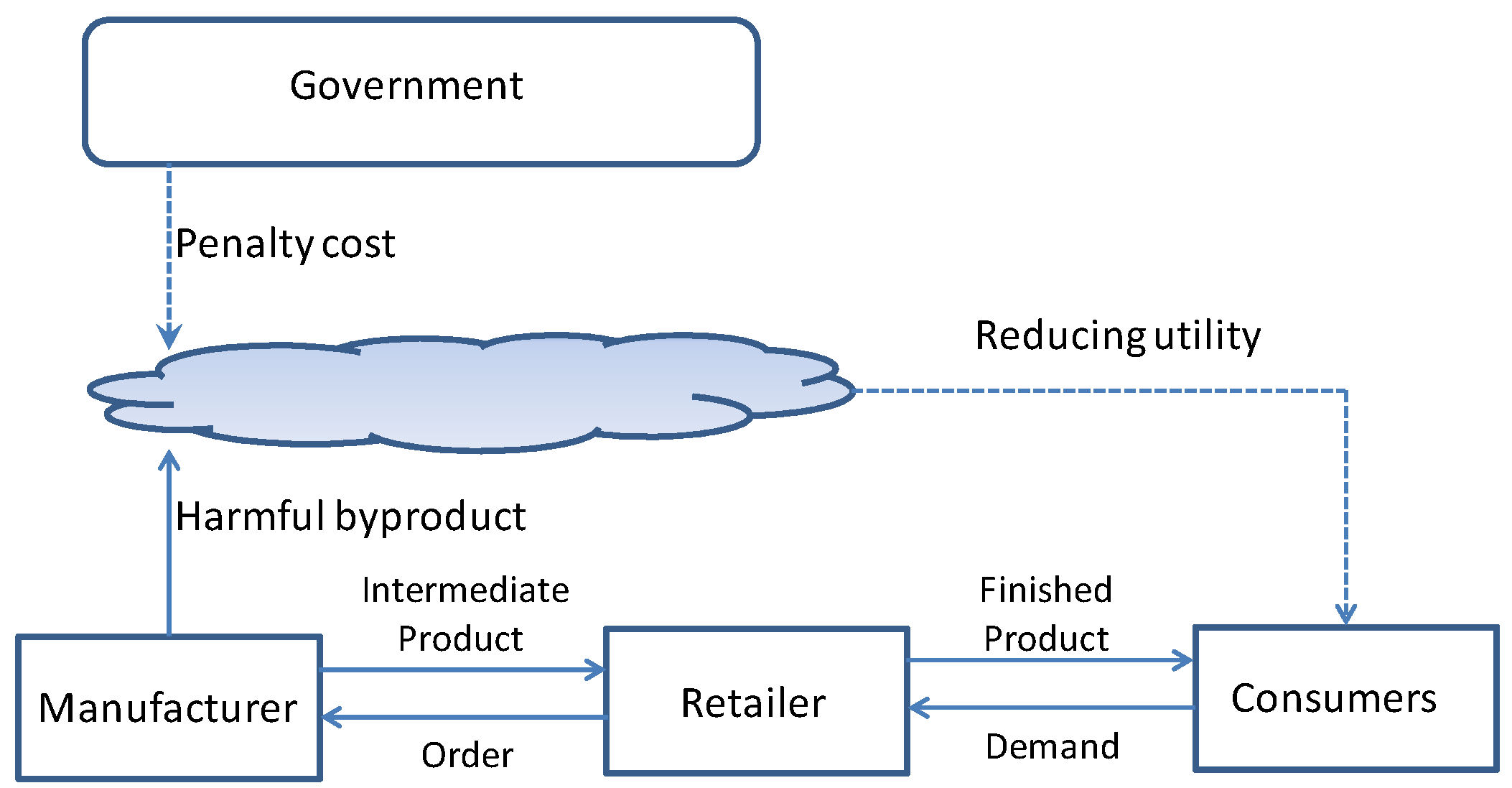
The setting of our research problem can be described as in
Figure 1. The supply chain consists of three primary players, manufacturer, retailer, and consumer. The manufacturer produces and sells its product to the retailer, who in turn sells the product to the end consumer. It is the manufacturer that emits pollution during the production process, which causes the environment to deteriorate [
29,
35]. The government imposes penalty on the manufacturer for its pollution emission.
In this context, we focus on two dimensions,
i.e., supply chain coordination and consumer awareness. There are two different supply chain coordination modes, competitive and cooperative. Under the competitive supply chain coordination, each of the two supply chain participants,
i.e., manufacturer and retailer, makes its own decision so as to maximize its own profit. On the contrary, under the cooperative supply chain coordination, the two participants are making a decision as if both belong to the same decision-making entity,
i.e., they have one objective function combining their profits together. In addition, we consider two types of consumer, one who is aware of,
i.e., sensitive to, the pollution emitted by the manufacturer and the other who is ignorant of,
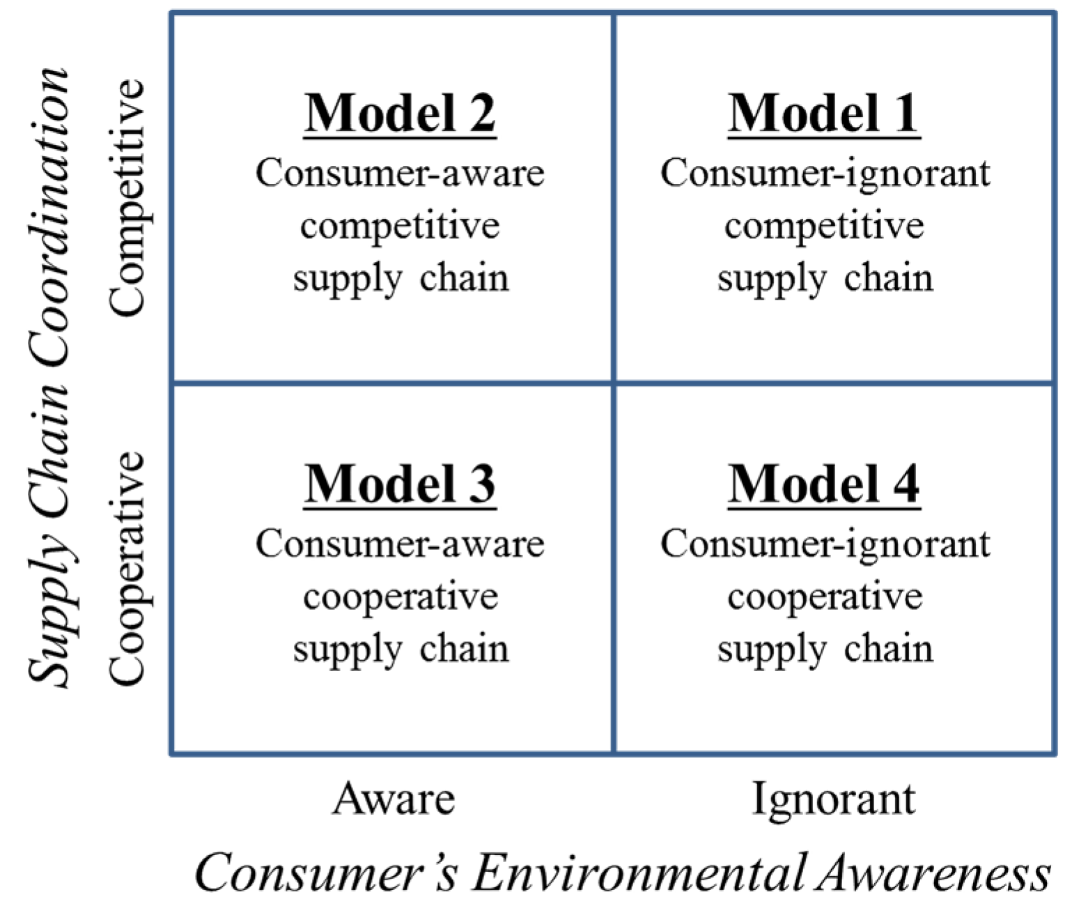
i.e., insensitive to, that. If the consumer is aware of and sensitive to the pollution emitted by the manufacturer, she will take into account the pollution level when making a purchasing decision. That is, the consumer’s demand function is affected by the level of the pollution stock. Using these two dimensions, we develop and analyze four models (
Figure 2), ignorant consumer and competitive supply chain (Model 1), aware consumer and competitive supply chain (Model 2), aware consumer and cooperative supply chain (Model 3), and finally, ignorant consumer and cooperative supply chain (Model 4). In addition, without loss of generality, we assume that there is little information or time gap between supply chain players, e.g., the retailer places an order, which is exactly the amount demanded by the consumers, the manufacturer produces the exact amount ordered by the retailer, and all of these ordering, producing, and delivering occur within the same sales cycle.
The major variables and parameters in the models are described in
Table 1. As the base case, we consider Model 1, where consumers are ignorant of the environmental issues and the supply chain is competitive. First, the retailer’s objective function writes:
In Equation (1),
,
, is the total net profit for the retailer, where
is the unit profit, sales price minus transfer price paid to the manufacturer, and
is the demand function,
i.e., the consumer’s demand for the retailer’s product is a function of the sales price,
, charged by the retailer. A quadratic cost function is assumed so that
is the total cost required for the retailer to process
units,
i.e., to finalize or refine the semi-finished products from the manufacturer to sell them to the end consumers. A quadratic cost function is widely used in the literature to represent the effect of increasing marginal cost (e.g., [
36,
37,
38]). Similar argument can be made to retailer’s processing cost, for instance, due to the need of having more expensive resources for processing as the volume increases. This assumption,
i.e., quadratic form of retailer’s processing cost, is often made in the literature (e.g., [
39,
40]).
Similarly, the manufacturer’s objective function writes:
The manufacturer’s total net profit is
, where
c denotes the unit production cost. In addition to the production cost, a cost incurs in a quadratic pattern as the production amount deviates from the manufacturer’s effective capacity,
: the more the production amount deviates from the effective capacity, the larger the quadratic cost,
i.e.,
. While producing the product, the manufacturer emits pollutants harmful to the environment:
y is the stock of pollution accumulated by
t. The government imposes a penalty on the pollution stock,
i.e.,
. The assumption of increasing convex cost on firm’s pollution is often used in the literature that studies environmental sustainability (e.g., [
29,
41]). It also implies that pressures from a regulator increase more than proportionally with pollution amount. Weil [
42] showed that larger firms, typically generating larger pollution, not only have higher probabilities of being subject to regulator’s inspections, but also pay substantially higher fines per violation of sustainability standards than small firms. Similarly, Gray and Shadbegian [
31] showed that regulators conduct more pollution-related inspection and enforcement to larger plants. The recent decision of China to impose fines total 26 million dollars to six companies about their pollution violations, the biggest environmental pollution case in China, also supports this assumption [
43]. In order to reduce the government’s penalty, the manufacturer makes an effort to cut its emission of pollutants. The effort level is denoted as
v and an associated cost incurs in a quadratic way like
[
29,
44].
Both the manufacturer and the retailer maximize their objectives subject to the common constraint:
Note that the common constraint, known as a state equation, between players is a distinguishing feature of a differential game and it implies that both players have the possibility of being influenced by the state of the system (
i.e., pollution stock in this paper) over the planning horizon in determining their actions. If the manufacturer does not make any effort to reduce the pollution, it emits pollution as much as
at
t,
i.e., the amount of pollution emission is proportional to the manufacturer’s capacity [
31,
32,
33]: one unit of capacity emits
l units of pollution. If the manufacturer’s effort level to reduce the pollution is
v, one unit of capacity emits only
units of pollution. The pollution stock
y decays naturally by
δy at
t: that is, the nature has a certain level of power to decompose and neutralize the pollutant, depending on its carrying capacity [
45,
46]. Now we have the dynamic evolution of pollution stock as
. We recapitulate the differential games for Model 1 as follows:
Model 1:
Retailer’s objective writes:
Manufacturer’s objective writes:
Now let us consider Model 2, which is different from Model 1 in one aspect: Model 2 assumes the consumers are aware of and sensitive to the pollution emitted by the manufacturer, whereas Model 1 assumes the consumers are ignorant and insensitive. How can we model the consumer’s awareness? In order to incorporate the consumer’s awareness of the pollution, we change the demand function so that it is now a function of not only the sales price, but also the pollution stock,
i.e.,
, where
γ is the demand function’s coefficient associated with the pollution stock. Similar demand function has been used in the work of Hovelqaue and Bironneau [
47] and the work of He
et al. [
44]. We provide the decision problems as follows.
Model 2:
Retailer’s objective writes:
Manufacturer’s objective writes:
Model 3 is different from Model 2 in that the manufacturer and the retailer coordinate with each other closely as if they were a single company,
i.e., it is the cooperative supply chain. Now there is only one objective function to be maximized by the integrated decision-maker combing the manufacturer and the retailer. The objective function for the cooperative supply chain is written as follows:
which is the combination of Equations (8) and (9) after canceling out
.
Model 3:
Finally, Model 4 is different from Model 3 in that the consumers are ignorant of and insensitive to the manufacturer’s pollution stock. Therefore, the demand function is now independent of the pollution stock, i.e., now the demand function is instead of .
Model 4:
We present the detailed solution procedure for Model 2 in
Appendix A: note that the solutions for other models are similar with that for Model 2. We summarize the analysis results of the long-term equilibrium for the four models in
Table 2.
4. Theorems
Based on the analysis of the differential game models, we develop theorems for the long-term equilibrium,
i.e., the long-term equilibrium behaviors of the factors that determine the firm’s dynamic decision making to reduce the pollution.
Theorem 1. At the long-term equilibrium, the manufacturer’s effort to reduce its pollution (v) and the accumulated pollution (y) are identical for Model 1 and Model 4. That is, and .
Theorem 1 implies that when the consumers are ignorant of and insensitive to the manufacturer’s pollution emission, whether the supply chain is cooperative or competitive does not make any difference to the manufacturer’s effort to reduce pollution and the ensuing accumulated pollution level.
Theorem 2. There exists a transfer price
such that
Theorem 2 examines the pollution dynamics of the consumer-aware competitive supply chain, according to the transfer price. In a competitive supply chain, how to set a transfer price is an important mechanism to coordinate various decisions of the manufacturer and the retailer within the supply chain [
18,
48,
49,
50].
As rearranging the Equation (18) yields
, we infer that
is less than the unit production cost
c when
is large compared with other parameters. Consequently,
holds given sufficiently large
, since it is reasonable to assume that the manufacturer would charge a transfer price
to the retailer that is higher than its unit production cost
c,
i.e.,
. Therefore, we infer that when the capacity is relatively large, the long-term cumulative pollution of Model 2, the consumer-aware competitive supply chain, is smaller than that of Model 1 and Model 4. Similarly, we deduce that when the capacity is relatively large, the manufacturer’s long-term effort to reduce pollution in Model 2, the consumer-aware competitive supply chain, is larger than that in Model 1 and Model 4. That is, under a normal situation, the manufacturer makes more effort to reduce pollution when the consumers are aware of and sensitive to the pollution stock and the supply chain is competitive than when the consumers are ignorant of the pollution.
Theorem 3. There exists a market potential level such that and , if Theorem 3 investigates the consumer-aware cooperative supply chain in terms of pollution emission, according to the potential market size. The potential market size directly influences the payoff in the supply chain, thus having a huge impact on the decisions including optimal emission and abatement in the supply chain [
12,
27].
In addition, from the long-term equilibrium derived in
Table 2, we know that the long-term demand in Model 3 remains positive if and only if
. Therefore, we infer that in general
holds and the long-term cumulative pollution of Model 3, the consumer-aware cooperative supply chain, is smaller than that of Model 1 and Model 4.
Similarly, we deduce that in general the manufacturer’s long-term effort to reduce pollution in Model 3, the consumer-aware cooperative supply chain, is larger than that in Model 1 and Model 4. That is, under a normal situation, the manufacturer makes more effort to reduce pollution when the consumers are aware of and sensitive to the pollution stock and the supply chain is cooperative than when the consumers are ignorant of the pollution.
Theorem 4. It holds that and , where i = I, II, III, IV.
Theorem 4 implies that as the government’s penalty on the manufacturer’s pollution stock increases, the manufacturer makes more effort to reduce the pollution and therefore the pollution stock decreases. Another route from the government’s penalty to the reduction of the pollution stock is more direct, i.e., the government’s penalty directly affects the manufacturer’s profit function.
5. Numerical Examples
To visualize the analysis outcomes, we conduct numerical analysis. Parameter values for the base case are in
Table 3. These values are based on the smartphone manufacturing industry in Korea: (1) the transfer price of a smartphone is about $500 per unit (
p1 = 50) and the unit production cost of a smartphone is about $200 per unit (
c = 20); (2) one unit of manufacturer capacity emits 0.01 ton of pollution (
l = 0.01); and (3) the potential market size is about 2,000,000 units per month (
α = 200,000. Accordingly, the major variables are interpreted as follow: the measure of manufacturer’s pollution accumulation (
y) is 10 tons, the measure of sales price is $10 per unit, and the measure of manufacturer’s pollution abatement effort (
v) is ton per unit capacity.
Table 4 summarizes the long-term equilibrium values of the variables and profits for the four models. It shows that Model 1 and Model 4 end up with the largest pollution accumulation (
y) along with the least effort to reduce the pollution (
v). This is generally consistent with the first three theorems. That is, in terms of pollution reduction, the consumer-ignorant supply chain performs much worse than the consumer-aware supply chain does. However, purely from the consumer welfare’s perspective, the consumer-ignorant cooperative supply chain,
i.e., Model 4, performs much better than others except for Model 3, the consumer-aware cooperative supply chain. That is, under Model 4 and Model 3, the equilibrium sales price is the lowest and the market demand per period is the largest. This result is consistent with the literature,
i.e., the cooperative supply chain is better for the market since it eliminates double marginalization. Similarly, the two cooperative supply chains,
i.e., Model 3 and Model 4, perform better in terms of the supply chain profits. That is, under Model 3 and Model 4, the supply chain profit, which sums the retailer’s profit and the manufacturer’s, is the largest. Again this result is consistent with the literature, which supports that the cooperative supply chain generates more profit for the entire supply chain than the competitive supply chain does. Of course, this does not imply that Model 3 and Model 4 are fairer for the supply chain partners than Model 1 and Model 2. Whether the cooperative supply chain is fairer or not depends on how to share the increased profit between supply chain partners. Now, which supply chain is the best? First, from the consumer welfare’s perspective and also from the supply chain profit’s perspective, Model 3 and Model 4 are better than the others. In addition, between Model 3 and Model 4, Model 3 is more desirable then Model 4, since it generates the least amount of pollution.
Let us consider more details of the numerical analysis.
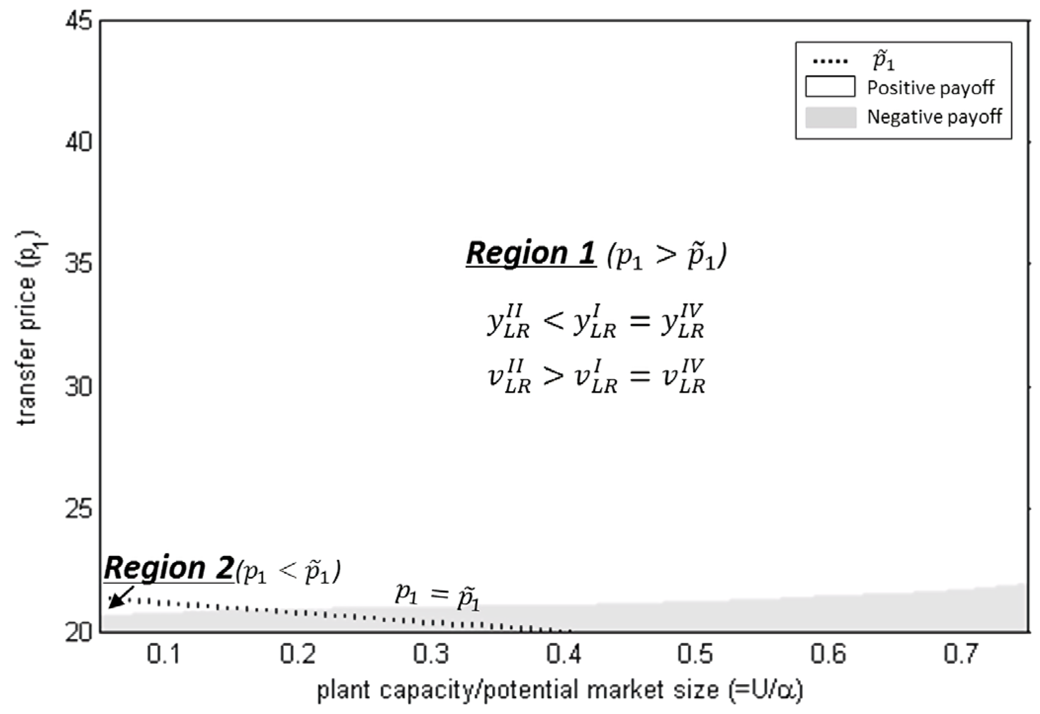
Figure 3 illustrates the dynamics of cumulative pollution and pollution abatement effort in the consumer-aware competitive supply chain compared with the consumer-ignorant supply chains. In
Figure 3, there are two regions: Region 1 (
) implies that the consumer-aware competitive supply chain emits smaller pollution and invests more in pollution abatement than the consumer-ignorant supply chains and Region 2 (
) shows the reverse. However, as shown in
Figure 3, the consumer-aware competitive supply chain outperforms the consumer-ignorant supply chains in terms of environmental performance in most cases (
i.e., Region 1 is much larger than Region 2), where the transfer price and the plant capacity are sufficient enough to guarantee a positive payoff for the manufacturer. It is unlikely to observe Region 2, where the consumer-aware competitive supply chain leads to a larger emission and a smaller abatement effort than the consumer-ignorant supply chains do, except for some extreme cases, where the plant capacity is very small compared to the market size and the transfer price is also very low.
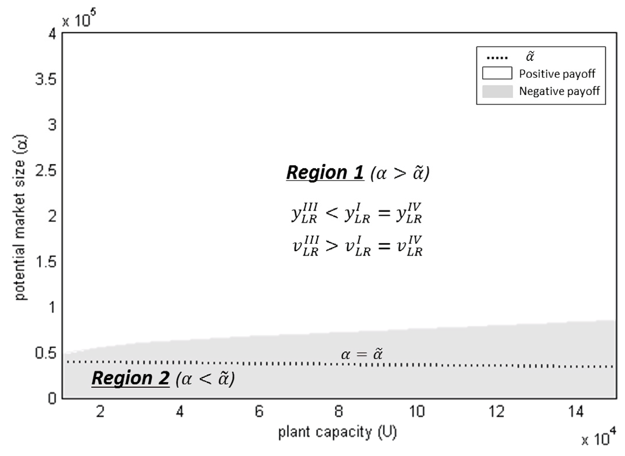
Figure 4 compares the consumer-aware cooperative supply chain and the consumer-ignorant supply chains. It shows two regions,
i.e., one with the potential market size larger than
(Region 1) and the other with the potential market size smaller than
(Region 2). Consistent with Theorem 3, the cumulative pollution is smaller and the pollution abatement effort is larger in the consumer-aware cooperative supply chain than the consumer-ignorant supply chains, provided that the potential market size is large enough to yield a positive payoff and also a positive demand for the supply chain. Intuitively, the cooperative supply chain earns a larger profit by eliminating double marginalization, thus allocating more resources to the abatement effort when the consumers are aware of the firm’s environmental performance. When the potential market size is smaller than
, the consumer-aware cooperative supply chain might emit more pollution and invest less in the abatement than the consumer-ignorant supply chains. However, this circumstance is not sustainable, since such a low potential market size would ultimately put the supply chain out of business in the long-term, it would not be profitable for the firm to be in such a market.
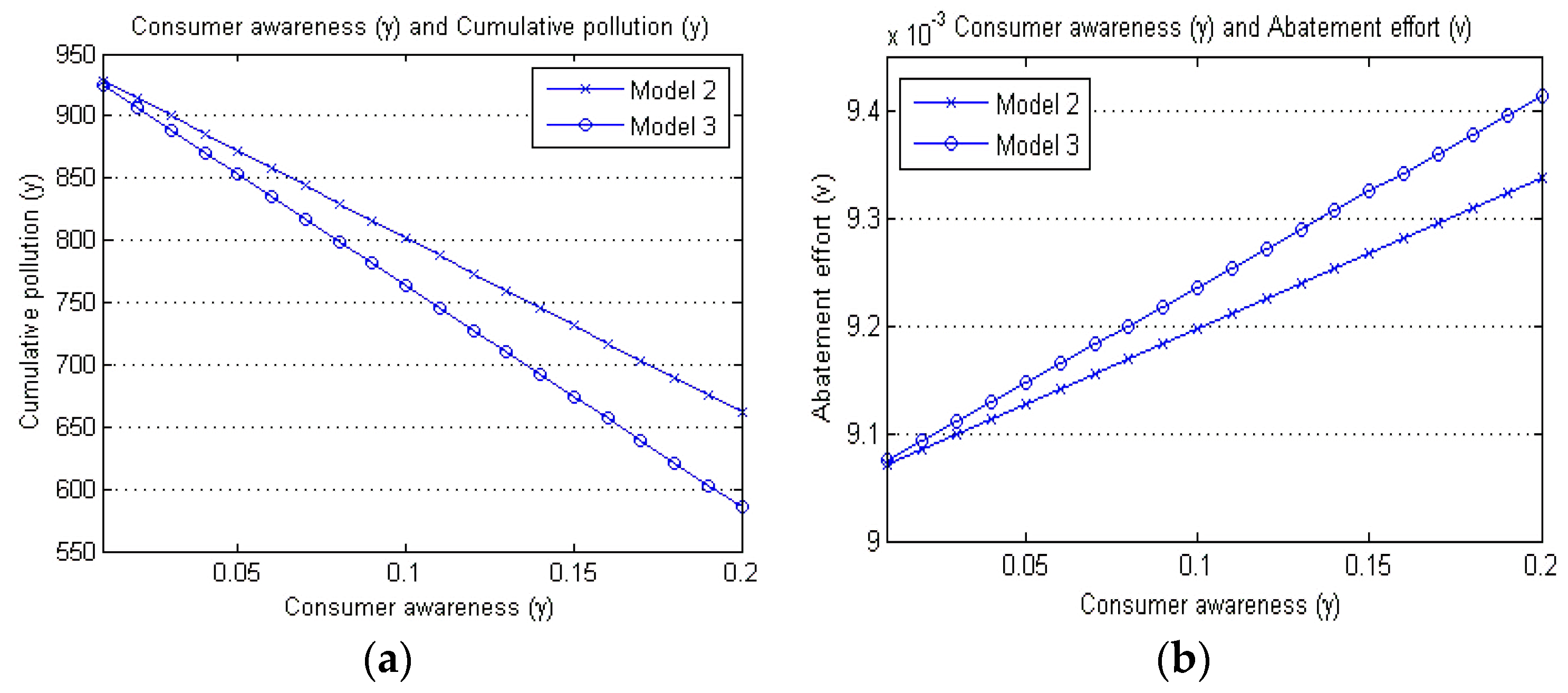
Comparing Model 2 and Model 3,
Figure 5 shows how the consumer’s environmental awareness influences the firm’s pollution abatement effort and cumulative pollution for the consumer-aware supply chains. As proved in Theorem 1, in the consumer-ignorant supply chains, the supply chain coordination (
i.e., competitive
vs. cooperative) has little to do with the firm’s abatement effort and pollution emission. In the consumer-aware supply chains, however, it has a significant impact on the pollution related decisions—the manufacturer in the competitive supply chain invests less in its abatement activity and thus emits more pollution than in the cooperative supply chain. However,
Figure 5 indicates that the effect of supply chain coordination is relatively insignificant when the consumer’s environmental awareness is low. That is, even in the consumer-aware supply chains, the supply chain coordination results in a significant difference in terms of the firm’s emission and abatement behaviors, only when the consumer awareness is sufficiently high. For instance, in
Figure 5a, the cumulative pollution (
y) of Model 3 is about 98% of that of Model 2 when the consumer awareness is relatively low, e.g.,
γ = 0.05, whereas it is less than 93% when the consumer awareness is relatively high, e.g.,
γ = 0.15. This strongly confirms the important role played by the consumer’s environment awareness in curbing the firm’s pollution emission.
6. Discussion and Conclusions
In this section, we further elaborate on each theorem. Theorem 1 highlights the importance of consumer awareness in reducing the pollution emitted by the manufacturer. It is well known that whether the supply chain participants are competing or cooperating with each other affects the consequences of supply chain strategy to a great extent. However, our analysis strongly indicates that unless the consumers are aware of and sensitive to the pollution, i.e., taking into account the pollution when making their purchasing decision, there is no difference between the two supply chain coordination strategies, i.e., competitive and cooperative, in influencing the manufacturer to reduce its pollution emission.
Theorem 2 puts forth that a sufficiently large transfer price from the retailer to the manufacturer ensures that the consumer-aware competitive case is better than the consumer-ignorant cases in reducing the pollution. It also implies that if the transfer price is excessively low, it gives the manufacturer little incentive to make an effort to reduce the pollution, leading to less investment in pollution abatement effort and therefore more accumulated pollution stock.
Theorem 3 shows that the consumer-aware cooperative case is better than the consumer-ignorant cases as long as the potential market size is sufficiently large. By proving that such a condition should hold in order for the long-term demand to be positive, it actually confirms that the consumer-aware cooperative case is always better than the consumer-ignorant ones in reducing the pollution, under normal market conditions.
Finally, Theorem 4 clearly demonstrates that the government penalty is effective for each of the four cases, implying that when executed properly, the government penalty can play an important and effective role in curbing the environmental degradation due to the pollution emission in the supply chain.
We have conducted a numerical analysis to visualize the implications of the theorems. The numerical outcomes are consistent with the theorems. One intriguing observation is concerned with the comparison between the consumer-aware cooperative and the consumer-aware competitive supply chain. As expected, the cooperative supply chain performs better than the competitive counterpart. However, the magnitude of its advantage enlarges as the level of consumer awareness increases. As discussed already, this observation further highlights the key role played by the consumer awareness in reducing the pollution emission.
Our research offers significant economic as well as managerial insights. First of all, Theorem 1 sheds light on understanding the essential role played by the consumers in controlling the pollution in a supply chain. It makes a potentially significant contribution to the literature by postulating a theory, which seems to contradict other existing ones in the literature. That is, the literature suggests that a cooperative supply chain performs better than a competitive supply chain or at least that the two supply chains, i.e., competitive and cooperative, generate different outcomes in most cases. However, our first theorem puts forth that the two supply chains, competitive and cooperative, are not different in terms of pollution reduction, unless the consumers are fully aware of the harmful effect of the pollution and take it into account when making their purchasing decisions. Stated differently, an elimination of double marginalization in a supply chain improves supply chain efficiency in terms of profit, but it alone cannot be a complete solution to environmental issues in a supply chain if it is not accompanied by proper change in a broader society (e.g., mindset of consumers). Therefore, reducing pollution and improving environmental sustainability in a supply chain should be approached from a perspective of entire economic system than the supply chain only.
It is also insightful that the transfer price determines whether the consumer-aware competitive case performs better in reducing the pollution than the consumer-ignorant cases. We conjecture in most situations, the transfer price is high enough to make the consumer-aware competitive case perform better than the consumer-ignorant cases. Nevertheless, it is not impossible for the consumer-ignorant cases to perform better than the consumer-aware competitive case if the transfer price is excessively low and thus the manufacturer has little motivation to make an effort to reduce the pollution. It also alludes to the retailer’s role to curb pollution of upstream manufacturer in the supply chain. For instance, a retailer might be able to influence manufacturer’s payoffs and incentives for abatement by negotiating the transfer price with the manufacturer. This role of retailers, or intermediaries in general, would have more impact when upstream manufacturers do not fully take into account end consumer’s awareness in their decisions. For example, a supplier that provides LCD panel to a TV set manufacturer might not be well aware of end consumer’s awareness (e.g., care about carbon footprint of a supply chain). In such circumstances, the intermediary (the TV set manufacturer here) might impact upstream supplier’s incentives for pollution abatement via negotiating the transfer price. We believe that the role of these intermediaries in improving environmental sustainability in supply chains deserves a closer examination in future research.
For the consumer-aware cooperative case, the analysis result is much stronger. Although the analysis shows that the potential market size determines whether the consumer-aware cooperative case performs better than the consumer-ignorant cases, it turns out that in order to have a feasible solution, i.e., under any possible realistic situations, the consumer-aware cooperative case always performs better in curbing the pollution than the consumer-ignorant cases.
Finally, it is intriguing to note that the government penalty always forces the firm to increase its investment in pollution abatement and thus to reduce the accumulated pollution stock, regardless of whether the supply chain is competitive or cooperative and also whether the consumers are aware or ignorant. In this light, the government policy seems to be an effective tool to control the pollution. Nevertheless, this observation does not necessarily mean that the government penalty is a tool more effective than the consumer’s environmental awareness. In fact, it can be a good topic for future research.
We believe our research helps both government policy makers and managers understand the complicated dynamics among critical factors related with consumers and supply chain strategies so as for them to make a decision to control the pollution more effectively. In essence, it strongly suggests that to reduce the pollution, managers and policy makers should try two methodologies simultaneously, one to encourage more coordination in the supply chain and the other to educate and/or motivate consumers to be more active for the environmental causes.
In this paper, our primary interest lies in the impact of consumer awareness and supply chain strategies on the environmental sustainability. However, we also believe that there might be other factors that influence the dynamics of pollution accumulation and abatement efforts in the supply chain. One of such factors includes bargaining power in a supply chain, which vary across industries, products, and exchange relations. For instance, different bargaining power structure would create different patterns in how the transfer price is determined, thus influencing incentives for pollution abatement in the supply chain. Incorporating the bargaining power issues to our study will not only improve practical relevance of the analysis, but also bring new insights to managers and policy makers. Furthermore, an empirical research that investigates the combined effects of supply chain strategies and consumer awareness on firm’s environmental performance using multiple cases or large-scale data across industries will provide a good opportunity to validate and compare the implications of this study.


