Historic Food Production Shocks: Quantifying the Extremes

Abstract

Understanding global food production trends is vital for ensuring food security and to allow the world to develop appropriate policies to manage the food system. Over the past few years, there has been an increasing attention on the global food system, particularly after the extreme shocks seen in food prices after 2007. Several papers and working groups have explored the links between food production and various societal impacts however they often categorise production shocks in different ways even to the extent of identifying different levels, countries and timings for shocks. In this paper we present a simple method to quantify and categorise cereal production shocks at a country level. This method can be used as a baseline for other studies that examine the impact of these production shocks on the global food system.

1. Introduction

Production of food has changed dramatically over the last century. New crops, expanded growing areas and better agricultural practices and technology have contributed to a significant increase in the total volume of food produced each year. Indeed, in a world with a population that has more than trebled over that time obesity is a major global challenge.

However, the world now faces a number of challenges in continuing to meet food demand over the next century [1,2]. These challenges include a rising population, changes to diet and environmental degradation impacting the productivity of land. Climate change represents a particular challenge to the global food system. Several studies of the impact of climate change on agriculture over a medium to long period of time (see, for example, [3,4]) highlight the need for further research into this area as the impact of temperature, carbon dioxide fertilization, the ability of farms to adapt and the specific adaption pathways currently leave a large range of potential impacts on food production capacity.

Some studies show that by the end of the century there could be a significant short fall in total food availability while others show there could be an increase. Many of these studies also only explore the average (mean) impact of temperature and weather changes while extreme weather events that can have a potentially significant impact on food output are not accounted for. Certain extreme weather events will be significantly impacted by climate change in the future (see, for example, [5]).

Over a shorter time frame there is increasing evidence that extreme weather events are becoming more frequent [6,7]. Drought, heat and extreme rainfall can have significant impact on crop productivity and therefore understanding the changing likelihood and shape of the probability distribution for these short term events is of increasing importance. However, a significant impact on crop productivity does not always translate into a shock in the global food supply system.

Global food supply is now a complex system. The interconnected nature of inter-country food dependence has increased dramatically over the last few decades [8]. A globalised market can make the system itself more resilient to localised shocks when food can be sourced from alternative places not experiencing the particular shock. However, if there are systemic linked events in different regions or across a wide region, or an event is of sufficient size, then this system can be perversely more fragile [9,10]. In particular the tele-connected nature of extreme weather events is becoming an increasing focus of research [9] and while the short to medium term dynamics are not well understood at present it is important to develop methods that can use the outputs of these models to assess potential social impacts.

These systemic risks involving significant global losses of food production could have major societal and economic impacts both through availability and price. Previous production shocks have been linked to major global events such as civil unrest and, in turn, major upheaval [11,12,13]. Understanding the historic causes and transmission of shock through to societal impact is key [14,15]. A recent study examining the evolution of trade networks over the period 1992–2009 concluded:

The global food system does exhibit characteristics consistent with a fragile one that is vulnerable to self-propagating disruptions. That is, in a setting where countries are increasingly interconnected and more food is traded globally over the (last two decades), a significant majority of countries are either dependent on imports for their staple food supply or would look to imports to meet any supply shortfalls.

[10]

A crop production shock results in a global food supply shock through trade and export restrictions [16,17]. The responses of markets and governments to production shocks have been the subject of numerous studies since the 2007/08 price shocks [18,19,20,21,22,23,24,25,26,27] and range from short term speculation to more fundamental changes in policies.

While food systems are both inherently local, particularly in the case of subsistence farming, and global a useful unit to explore production shocks is the country level. An extreme shock in food production will invariably involve a response by a government at country level [16,25] in an attempt to manage local price increases and the impact of the shock. Therefore, developing a detailed understanding of the impact of productions shocks would initially necessitate an analysis at country level to allow a comparison across different studies. While it has been noted previously that the impact of food production shocks on an individual country do not seem to be correlated with whether that country is a net food importer or exporter [11] local infrastructure and processes will of course play an important part including transport, storage, policy responses and subsidies [9]. A common method to identify production shocks is therefore a first step in assessing whether an extreme loss constitutes a risk for a particular country or not.

There is now a substantial effort underway in academic communities to better model the dynamics of the global food system. However, a pre-requisite to these endeavours is to understand past production shocks and their impacts. A common baseline to identify and quantify these past shocks in needed if different studies are to be compared. This paper attempts to present a method to quantify the size of previous global food production shocks to allow an agreed approach to their measurement and use. These production shocks can then be used as a basis for historic event analysis to aid with better model and parameter development in this space. The paper does not attempt to reproduce the work of others on physical climate or weather modelling to explore the underlying causes of these production shocks nor does it attempt to match individual loss events with past extreme events. Section 2 presents our method for defining production shocks. Section 3 presents the results and Section 4 discusses these results and the limitations of our method. Finally we present some conclusions.

2. Production Shock Quantification Method

In this section, we firstly outline the data availability at country level and detail a method to create a consistent database of country level food production trends. We then propose a method of quantification to be applied to this data to identify production shocks. Ideally our method leads to a list of countries who have experienced a food production shock and the year in which this production shock occurs. This then allows further research into particular shocks to start from the same basis which is the intention of the work presented in this paper.

Comparison of analysis of the impacts of food production shocks requires a similar assessment of the size of a particular shock. In this paper we outline an approach to quantifying two scales of food production shock—country level and global. While food production takes place at very local levels, understanding the impact of a physical food production shock on social systems usually involves modelling the impact on food prices. Changes in food price usually come as a supply-demand response through export markets [28,29,30,31] and, therefore, country level analysis is the most appropriate to study, at least initially.

We constrain our choice of food to cereals as defined by the Food and Agriculture Organization (FAO). Cereals are directly impacted by extreme weather events, through droughts, extreme rainfall and temperature, and quantifying this is a key first step in understanding future climate change impacts on food systems in general. We explore production shocks over annual cycles as a basis for the analysis.

As a baseline we look at global cereal production data over the past 17 years. We take data from the Food and Agriculture Organization Corporate Statistical Database (FAOSTAT) [32] for world cereal production from 1995 to 2011 and use this data to plot a linear regression line. Figure 1 shows the data and regression line for world cereal production. As can be seen this shows an increase in global cereal production over this period. If we assume that the trend line represents cereal production under normal conditions then deviations from this trend represent production gains due to ideal conditions or losses due to less favourable conditions. The standard deviation of the differences between the real (as reported in FAOSTAT [32]) and trend data is 3.84%. The largest production shock observed over this period was in 2002 with a 7.15% shock. Does 2002 represent a production shock? At what level should we categorise a production shock? Given global level data only and using this as a basis for trends it is difficult to see how an objective quantified measure based on statistical analysis is possible. Therefore, more detailed analysis on a country by country basis may offer a better method to define an objective statistical measure for production shocks.

To identify food production shocks, yearly cereal production data for 187 countries from 1995 to 2011 was taken from FAOSTAT [32] totaling 3197 data points. To quantify the size of a shock we first need to identify the underlying trend in production for a particular country.

From the data obtained, linear or polynomial regression lines for each of the countries’ time series were calculated depending on the trends in the data to minimize the coefficient of determination (R-squared). The form of the regression lines can be seen from Equations (1) and (2):

$$Linear regression: y_e= {\beta }_{1}x+c$$

(1)

$$Polynomial Regression: y_e= {\beta }_1{x}^2+{\beta }_{2}x+c$$

(2)

where $x$ is the year in the time series, ${\beta }_1$ and ${\beta }_2$ are coefficients of $x$, $y_e$ is the estimated production data and $c$ is a constant. The data obtained from these regression estimations smooths out any production shocks observed in the raw data. These trend lines are assumed to be the “normal” production for that country assuming no shocks.

A percentage difference between the raw data and the regression data for each country was then calculated. This was done in two ways—as a percentage of that particular country’s production and as percentage of global production, as seen in Equations (3) and (4):

$$D_C= \frac{\left(y_d- y_e\right)}{y_e}$$

(3)

$$D_T= \frac{\left(y_d- y_e\right)}{y_t}$$

(4)

where $D_C$ is the country level percentage difference, $D_T$ is the world level percentage difference, $y_d$ is the raw country production data point, $y_e$ is the regression estimation for that country in that year and $y_t$ is the sum of all the raw data points for one year in the time series—the total production of cereal globally in that year.

This gives us two tables with percentage of real observed cereal production away from “normal” production trends. These percentage deviations can be both positive—meaning a country has produced more cereal in a given year than its trend line, or negative—meaning a country has produced less cereal in a given year than its trend line. With no extreme production failures we would expect these production anomalies to follow a normal distribution around the mean trend lines. These trend lines, on average, have a positive gradient over this period of time meaning that global cereal production in 2011 is higher than it was in 1995. This is to be expected as food production has expanded over this period—both in terms of agricultural land and farming productivity. However, not all countries show an increase.

We then calculate the standard deviation of these percentage production anomalies. This standard deviation allow us to estimate the expected size of production changes year on year across countries. We exclude countries that have zero production, and therefore zero percentage production anomalies, so these values do not skew the standard deviations.

To explore shock events we assume a normal distribution in the underlying trend as a first approximation. A shock event is then defined as any deviation away from the trend line that has a significantly low probability of occurring. We take this point as falling outside of 99.7% of a normal distribution—that is 3 standard deviations. This roughly translates as an event with a recurrence of 1 in every 666 years if the distribution is truly normal.

Shocks, or “3 sigma events”, were therefore identified as data points that fall below three standard deviations from the estimated regression data for both country and global level shocks.

At country level this represents a significant shock for that country and allows us to classify shocks per country. However, these shocks may be insignificant on a global level but of course represent a significant local event. At global level the percentage anomalies and their distribution is much smaller than at country level. This is because it is possible for one country to experience a shock of more than 50% of its own production in any year whereas a particular country’s production contribution to global production is of course much smaller. Therefore a country level 3 sigma event is likely to represent a very significant loss in production for that country. The global food system experiences much smaller percentage production losses than individual countries due to the diversity of geographic growing areas.

Global shocks occur when a number of smaller countries, or a major producer, experience a shock at the same time. Given this, the anomalies each year for production shocks are likely to have a smaller distribution at global level and major producers will have a higher impact on global supply than other countries. However, those global production shocks may not represent a country shock in those major producers using our definition of a 3 sigma event. For example, the US and China are both major cereal producing countries and while a particular event in those countries may be under 3 sigma at country level it could still represent a higher than 3 sigma event at global level. If the US lost under 50% of its production, while this may not be categorized as a country level shock, it would represent a global shock in production.

By categorizing shocks both at country level and global level we ensure that any event which will have an impact on country level supply and demand from both the import and export perspective is still categorized as a shock. If a country is categorized as having a shock this then allows the researcher to further explore those particular events to determine whether that shock represents a political or social risk for those countries or elsewhere.

3. Results

Here, we present the results from applying the percentage anomaly calculations at both country and global levels. We then identify production shocks at country and global level and explore the difference between these two approaches.

Table 1. Country percentage difference from trend for a set of countries over the time series considered.

Country	1995	1996	1997	1998	1999	2000	2001	2002	2003	2004
Afghanistan	19.69	12.81	20.66	19.78	3.68	46.32	44.04	−4.86	6.9	17.59
Albania	2.35	−15.55	5.92	11.03	5.59	10.54	−0.48	3.62	−2.85	−2.11
Algeria	−3.25	111.22	64.19	19.13	23.7	66.14	−7.24	−34.4	38.25	26.22
Angola	16.68	30.57	1.31	25.19	1.61	11.82	−5.9	7.15	0.02	−6
Argentina	21.11	−2.36	11.68	15.37	3.98	13.59	3.13	10.28	−4.36	−2.93
Armenia	11.62	8.44	13.85	6.64	4.23	30.11	12.58	24.37	−8.47	33.16
Country	2005	2006	2007	2008	2009	2010	2011
Afghanistan	22.31	−0.34	20.64	22.18	26.39	11.23	16.29
Albania	−1.76	−5.32	11.46	4.23	2.5	6.3	1.12
Algeria	6.74	17.64	2.21	57.73	40.34	3.85	−5.91
Angola	9.69	20.32	21.81	21.46	2.58	9.48	24.52
Argentina	1.49	10.98	13.33	−7.65	34.83	14.76	17.16
Armenia	13.69	40.38	22.38	9.86	−2.98	16.89	10.25

shows an example of the country percentage $D_C$ for a set of countries.

The standard deviations of the two sets of percentage differences obtained were then calculated. This equates to 19% relative to a country’s own production and 0.2% relative to world production. Using the 3-sigma definition to identify a shock, at country level this corresponds to shocks in production of 58% while at global level this corresponds to an individual country contributing a shock of 0.6% to global production. An extreme shock is therefore identified for any country that experiences a drop of 58% or more away from trend or any country that contributes more than 0.6% global production drop below trend by itself.

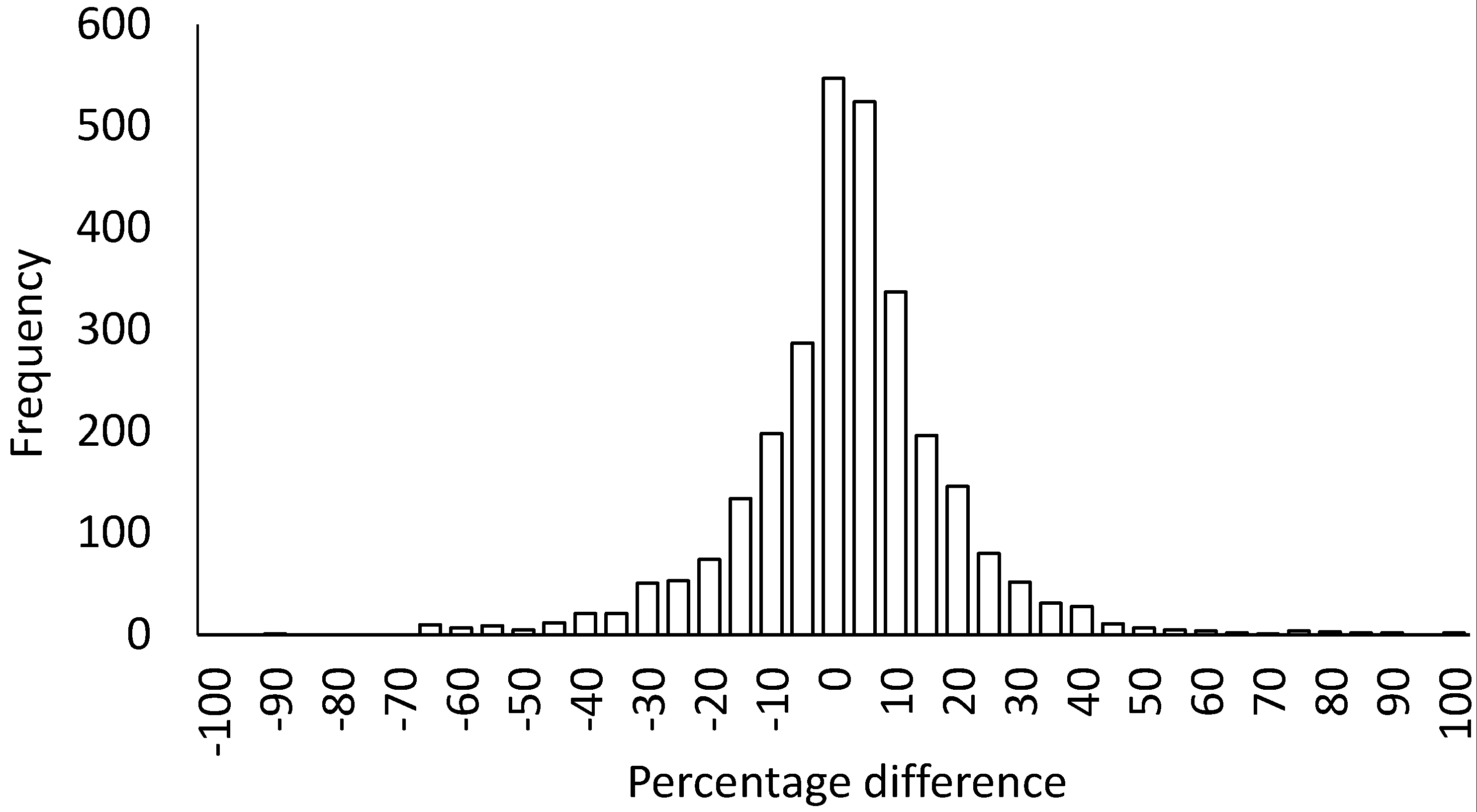
Figure 2 shows the distribution of percentage anomalies for country level production away from trend. As can be seen from the distribution at country level (Figure 2) there appears to be a small group of countries that do experience a significant shock event (larger than 58% loss in production) giving the distribution fat tails—a more common phenomenon in probability distributions such as this given the uncertainty of weather events [33]. Assuming a normal, or Gaussian distribution, will underestimate the frequency of these extreme “3 sigma events” which will be more common than in a normal distribution. However, the first approximation of a normal distribution for 3-sigma events is still valid as this is only used to identify extreme events for further analysis. We do not attribute likelihoods to those events but use them to explore further dynamics of the particular country production losses and how they impact on global food systems. To calculate probabilities of such events and the social consequences will require further analysis of the underlying distribution as well as assigning probabilities to the social responses to those events. This is out of the scope of the current paper.

Figure 3 shows the distribution of percentage anomalies for country level production as a contribution to global production away from trend. Due to the very small standard deviation compared to the furthest outliers in Figure 3, we use a logarithmic scale to represent the shape of the fat-tailed distribution. Although at global level (Figure 3) we see outliers where production deviating from a country trend line amounts to nearly −2% off global production, in fact the largest shock here is −3.45%, but these outliers are not displayed due to the logarithmic scale. Therefore, we see that a few events have contributed to significant shocks.

We then classify the particular countries that fall outside the 3-sigma event and the year in which the shock occurs. This classification allows us to produce a list of countries that we highlight as having experienced a production shock themselves or those that contributed to a shock in global production. The years that particular countries experienced production shocks given the two criteria are listed in

Table 2. Country level shocks.

Country	Year of Shock
Algeria	1997, 2000, 2008
Botswana	1998
Cape Verde	1997, 1998
Cyprus	1997, 2008
Fiji	1998
Iraq	2000
Jordan	1999
Kuwait	2007, 2008
Moldova	2007
Morocco	1995, 2000, 2007
Sao Tome and Principe	1998, 1999
Trinidad and Tobago	1999
Tunisia	2002

and

Table 3. Global level shocks.

Country	Year of Shock
Argentina	2009
Australia	2002, 2006
Canada	2002
China	2000–2005
India	2002, 2004
Russian Federation	1998, 1999, 2003, 2010
Ukraine	2003, 2007
United States	1995, 2001, 2002, 2006, 2011

.

Table 2 shows the countries experiencing significant shocks relative to their own production are usually not major producers. It instead highlights countries that experience the most variability in their annual food production are more likely to be smaller producers with less infrastructure and processes to manage major weather or political events that impact food production. These countries are less secure in their food availability and are more likely to need to increase their dependency on imports during these times of shock. Under usual conditions this may not represent a significant challenge however, if finance was a problem or their shocks coincided with a global shocks or import restrictions then this could represent a major potential impact on those countries. Furthermore, many of the nations identified are African and Middle Eastern states, arguably some of the most unstable parts of the world. There are production shocks in these nations in 1995, 1997, 1998, 1999, 2000, 2002, 2005, 2007 and 2008. If a major producer experienced a food production shock of 58% it would have catastrophic impacts on the global food supply system.

Table 3 shows the countries that experience the largest shocks relative to global production and are, as expected, the biggest producers. These production shocks ripple throughout the world’s food system and affect the producing country as well as all other countries that rely on their exports. Global shocks are experienced in every year except for 1996, 1997 and 2008.

Global production shocks are more often than not the result of a single country experiencing a production loss. However, if more than one major producer experiences a production shock then the global loss can be very high. For example, in 2002 there was a loss of 7.98% of all global cereals in that single year. Depending on what else is happening in the food system, in particular associated with stock levels, these global losses could lead to significant social impacts. At country level at least one country experiences a major shock (loss of more than 58% of its production) every other year.

Using purely global data (Figure 1) we also saw a production shock of 7.15% in 2002, which was less than a two sigma event using global only trend lines. However, using this new method we have shown that Australia, Canada, China, India and United States all having 3 sigma events in 2002 amounting to a 7.98% loss (the overall loss is slightly higher as the regression lines are done on a country by country basis and therefore the overall trend is slightly different to a global trend). In conducting this analysis we emphasise that it is the level of detail that is important and not the overall trend as displayed by the global data. Global 3 sigma events identified using country level data help identify where shocks took place, explaining possible re-orientations of the trading system of food.

4. Discussion

Rises in global food prices can have a significant impact on societies and have in the past led to social unrest [11,13]. However, the causes of food price rises are myriad [27] and the subject of a lot of study. One underlying cause is the physical availability of food. In particular shocks in cereal production are viewed as one of the causal factors in price shocks [16] although a cereal production shock does not always lead to a price shock and a price shock has not always been preceded by a production shock [9]. Never-the-less developing a policy response to food security and global food resilience requires a deep understanding of the food system.

Surprisingly there is no one agreed method for quantifying or categorizing when a country has experienced a food production shock. This paper has presented a linked method to categorize a country level production shock and a shock at country level that leads to a global production shock. We have identified several production shocks over the period 1995–2011 and classed these as country or global shocks while listing the year and country in which the shock originated.

Research which has explored the food system and price shocks can be better grounded in underlying production shocks by using this method. We argue that this would allow for an easier comparison between different arguments for causality of food price shocks. In particular in building quantified models having a similar basis for including cereal production shocks would create a better method for validation and calibration of these models. The simple formulation of identifying 3 sigma shock events presented in this paper should be readily reproducible by other research groups.

Of course several limitations exist with this method when using it for detailed policy development not least the quality of the data contained within the FAOSTAT database. Another key limitation is that food price shocks are rarely directly linked into overall cereal production but rather a complex interaction with imports, exports and stock levels. Also, as previously highlighted, this method does not identify whether a particular country is at risk of political or social impacts as a result of the production shock. The risk factors are myriad and include political responses, transport, storage infrastructure, substitutability of grains with other sources of food, exchange rates and food subsidies, However, we believe an initial categorization of food production shocks using this simple and common method will allow better cross-comparison between studies while given a common basis for further study into these more detailed responses to production shocks. This method should allow an identification of key countries to examine in further detail as potential sources of either shocks to import demand or export capability. Identifying a particular country of course is only the first step in understanding the dynamics of the global food system.

5. Conclusions

In this paper we present a method to categorize food production shocks at country level. We use data from FAOSTAT to list a set of extreme production shocks over the period 1995–2011 and the countries and years in which these shocks occur. We show that global cereal production shocks occur as a result of shocks in major cereal producers including USA, China, Russia, Ukraine, India, Argentina, Canada and Australia. The largest global shock using our method was a 7.98% shock in 2002. Production shocks when an individual country experienced more than 58% loss in annual cereal production has occurred 21 times during that period in countries that are predominantly classed as developing countries.

We argue that this method for categorizing annual cereal production shocks at a country level gives a common framework from which further investigations of the impact of such shocks can be built. Using this common definition for shocks, and the common list of countries contributing to these shocks, will make cross comparison between studies and methods more transparent in future. The cross comparison is important when using these models to inform policy decisions that are intended to better manage the global food system.