Optimal Energy Mix with Renewable Portfolio Standards in Korea

Abstract

Korea is a heavily energy-dependent country whose primary energy consumption ranks ninth in the world. However, at the same time, it promised to reduce carbon emission and planned to use more renewable energy. Thus, the objective of this study is to propose an optimal energy mix planning model in electricity generation from various energy sources, such as gas, coal, nuclear, hydro, wind, photovoltaic, and biomass, which considers more renewable and sustainable portions by imposing governmental regulation named renewable portfolio standard (RPS). This optimization model minimizes various costs such as construction cost, operation and management cost, fuel cost, and carbon emission cost while satisfying minimal demand requirement, maximal annual installation potential, and renewable portfolio standard constraints. Results showed that this optimization model could successfully generate energy mix plan from 2012 to 2030 while minimizing the objective costs and satisfying all the constraints. Therefore, this optimization model contributes more efficient and objective method to the complex decision-making process with a sustainability option. This proposed energy mix model is expected to be applied not only to Korea, but also to many other countries in the future for more economical planning of their electricity generation while affecting climate change less.

1. Introduction

The Republic of Korea, also known as Korea, is a heavily energy-dependent country because it ranks ninth in the world with respect to total primary energy consumption. However, it also depends highly on imports for its oil, coal, and natural gas consumption (second in liquefied natural gas imports, third in crude oil imports, fourth in coal imports, and sixth in dry natural gas imports) as it is not blessed with natural resources (43th in total primary energy production) [1].

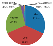
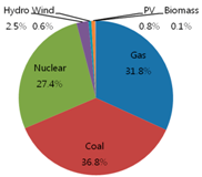
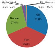
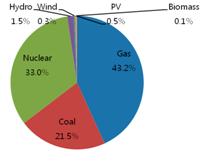
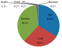
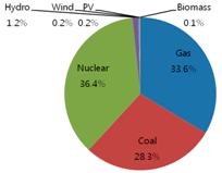
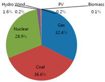
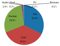
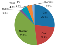
Although Korea consumes a lot of energy for its export-oriented industries, such as steel-making, ship-building, and car-making, it pledged to reduce carbon emissions [2] and it set a goal of using more renewable energy [3]. Additionally, after the Fukushima disaster in Japan, Korea is trying to moderate nuclear power generation targets [1]. Three identical pie charts in the second row of

Table 1. Optimal energy mix of Korean generation capacity.

Year	Optimization Model
	Basic	Basic + CO2 Cost	Basic + CO2 Cost + RPS
Initial (2011)
2020
2030

show the original energy mix of electricity generation in 2011 where gas accounts for 31.8%, coal 36.8%, nuclear 27.4%, hydro 2.5%, wind 0.6%, photovoltaic (PV) 0.8%, and biomass 0.1%, out of total 68.3 GW with respect to generation capacity. Additionally, three identical pie charts in the second row of

Table 2. Optimal energy mix of Korean generation amount.

Year	Optimization Model
	Basic	Basic + CO2 Cost	Basic + CO2 Cost + RPS
Initial (2011)
2020
2030

show the original energy mix of electricity generation in 2011 where gas accounts for 32.4%, coal 36.6%, nuclear 28.9%, hydro 1.6%, wind 0.2%, PV 0.2%, and biomass 0.1%, out of total 511 million MWh with respect to generation amount [4]. However, how to optimally mix those energy sources in the future while satisfying carbon emission limits and installing more renewable energy sources becomes a critical problem. Recently, Park et al. [5] proposed a bottom-up model (The Integrated Markal-Efom System model) for calculating the optimum renewable energy portfolio in the electricity generation sector of Korea. However, the model only focuses on the generation amounts of renewable sources, such as wind, PV, hydro, and geothermal. Thus, this study aims at developing an optimization model for the future energy mix problem in Korea, which calculates renewable energy amounts as well as fossil energy amounts.

So far, various energy mix or expansion optimization models have been developed [6,7,8,9,10] since a simple linear programming model was proposed [11]. Certain models considered the gap between long term investment and short-term operation [12], thermal operation in generation expansion planning [13], unit commitment constraint [14,15,16], and other issues, such as economics, finance, regulation, and uncertainty [17,18,19,20]. Furthermore, some optimization models have been applied to countries, such as Japan [21], Iberian countries of Portugal and Spain [22], and Mexico [23]. However, the full optimization formulations with full datasets were seldom provided, although certain endeavors exist [24]. Thus, this study also intends to provide full optimization information for other researchers to easily apply this model to their own energy mix problem.

2. Optimization Formulation

As mentioned above, Korea is a heavy energy consuming country while pledging to reduce carbon emissions. Thus, the country wants to optimally manage this problem in generating electric energy by considering various factors. Currently, Korea generates electricity from various conventional (gas, coal, and nuclear) and renewable (hydro, wind, PV, and biomass) sources. However, in order to attain the pledged goal of carbon emission reduction, it has to force more renewable amounts to be generated while considering various costs (construction, operation and management, fuel, and carbon emission costs), total electricity demand (including losses and reserves), annual renewable expansion capacity, and renewable portfolio standard (RPS) regulations.

The optimal energy mix model in this study is fundamentally based on the least-cost optimization model in previous research [4]. However, this model improves the formulation structure, uses updated data, and provides more explanatory computation results.

The objective function of the energy mix problem can be the total cost of electricity generation which consists of construction, operation and& management (O and M), fuel, and CO₂ costs as follows:

$$Cos{t}_{Total}=Cos{t}_{Const}+Cos{t}_{O\&M}+Cos{t}_{Fuel}+Cos{t}_{C{O}_2}$$

(1)

Since the energy mix policy is a multi-year one, we may introduce a discount factor [25] and each cost becomes as follows:

$$\begin{array}{l}Cos{t}_{Const}={\displaystyle \sum _e{\displaystyle \sum _{t=1}^T\left[\frac{1}{{\left(1+i\right)}^t}\times C_{Const}^e\times I_t^e\right]}},\\ e\in \{gas,coal,nuclear,hydro,wind,PV,biomass\}\end{array}$$

(2)

where $T$ denotes number of total project years (2012–2030 in this study), $i$ denotes discount rate (5% in this study [4]), $C_{Const}^e$ denotes the unit construction cost (US$/MW) of energy source $e$ (each energy source has different unit construction cost as shown in

Table 3. Construction, operation and management, and fuel costs by energy source.

Energy Source	Construction Cost ($/MW)	O and M cost ($/MWh)	Fuel Cost ($/MWh)
Gas	673,000	4.45	40
Coal	929,000	4.04	110
Nuclear	1,924,000	9.68	4
Hydro	3,951,700	18.81	0
Wind	3,498,000	22.12	0
PV	4,600,000	40.38	0
Biomass	4,334,000	48.05	24

[26,27], and $I_t^e$ denotes installed capacity (MW) of energy source $e$ in year $t$.

$$\begin{array}{l}Cos{t}_{O\&M}={\displaystyle \sum _e{\displaystyle \sum _{t=1}^T\left[\frac{1}{{\left(1+i\right)}^t}\times C_{O\&M}^e\times Q_t^e\times {\mathsf{\tau }}^e\right]}},\\ e\in \{gas,coal,nuclear,hydro,wind,PV,biomass\}\end{array}$$

(3)

where $C_{O\&M}^e$ denotes unit O and M cost (US$/MWh) of energy source $e$ (each energy source has different unit O and M cost as shown in Table 3 [26,27], $Q_t^e$ denotes cumulative generation capacity (MW) of energy source $e$ in year $t$, and ${\tau }^e$ denotes the capacity factor (h) which represents utilized hours of energy source $e$ in a year (each energy source has a different capacity factor as shown in

Table 4. CO₂ emission rate, capacity factor, and initial capacity by energy source.

Energy Source	CO2 Emission Rate (t/MWh)	Capacity Factor (h)	Initial Capacity (MW)
Gas	1.154	7621	21,740
Coal	1.965	7446	25,128
Nuclear	0.631	7884	18,715
Hydro	0.234	4642	1717
Wind	0.127	2890	406
PV	0.057	2190	554
Biomass	0.793	7271	96.8

[28] and maximum hours in a year are 8760 h). Here, it should be noted that the original formulation of Ahn et al. [4] omitted the capacity factor while it considered generation-hour-based O and M cost. In order to give consistency, the formulation in this study has the capacity factor.

$$\begin{array}{l}Cos{t}_{Fuel}={\displaystyle \sum _e{\displaystyle \sum _{t=1}^T\left[\frac{1}{{\left(1+i\right)}^t}\times C_{Fuel}^e\times Q_t^e\times {\mathsf{\tau }}^e\right]}},\\ e\in \{gas,coal,nuclear,hydro,wind,PV,biomass\}\end{array}$$

(4)

where $C_{Fuel}^e$ denotes the unit fuel cost (US$/MWh) of energy source $e$ (each energy source has a different unit fuel cost as shown in Table 3 [29].

$$\begin{array}{l}Cos{t}_{C{O}_2}={\displaystyle \sum _e{\displaystyle \sum _{t=1}^T\left[\frac{1}{{\left(1+i\right)}^t}\times C_{C{O}_2}\times Q_t^e\times {\mathsf{\tau }}^e\times R^e\right]}},\\ e\in \{gas,coal,nuclear,hydro,wind,PV,biomass\}\end{array}$$

(5)

where $C_{C{O}_2}$ denotes the unit CO₂ cost (7.4 US$/tCO₂ in this study and $R^e$ denotes the emission rate (tCO₂/MWh) of energy source $e$ (each energy source has a different emission rate as shown in Table 4 [30]. Here, it should be noted that the original emission rate data of Ahn et al. [4] appeared abnormally high. Thus, the original values were scaled down by multiplying the values by 10⁻³, which results in a reasonable range.

The total cost of electricity generation can be again expressed as follows:

$$\begin{array}{l}Cos{t}_{Total}={\displaystyle \sum _e{\displaystyle \sum _{t=1}^T\left[\frac{1}{{\left(1+i\right)}^t}\times \left(C_{Const}^e{I}_t^e+C_{O\&M}^e{Q}_t^e{\mathsf{\tau }}^e+C_{Fuel}^e{Q}_t^e{\mathsf{\tau }}^e+C_{C{O}_2}{Q}_t^e{\mathsf{\tau }}^e{R}^e\right)\right]}},\\ e\in \{gas,coal,nuclear,hydro,wind,PV,biomass\}\end{array}$$

(6)

Now that we have covered the objective function of the energy mix optimization, let us move on to the constraints. The first constraint can be minimal supply requirement for satisfying electricity demand as follows:

$$\begin{array}{l}{\displaystyle \sum _e\frac{Q_t^e\times {\mathsf{\tau }}^e}{1+k}}\ge \mathsf{\psi }{\displaystyle \sum _{Sector}{D}_t^{Sector}},\\ e\in \{gas,coal,nuclear,hydro,wind,PV,biomass\},\\ Sector\in \{industrial,residential,commercial\}\\ t=1,\dots ,T\end{array}$$

(7)

where $k$ denotes the loss factor due to transmission loss and internal electricity use (6% in this study), $\mathsf{\psi }$ denotes the level of the electricity supply target as a buffer (1.1 in this study), $D_t^{Sector}$ denotes the estimated electricity demand for each sector in year $t$. $D_t^{Sector}$ data can be obtained from various sources or calculated using the annual demand growth rate. This study follows the tabulated data in previous research [4]. Here, it should be noted that the original formulation used $\left(1+k\right)$ in Equation (7); however, this study uses ${\left(1+k\right)}^{-1}$ because the generation amount, including the loss amount, should be greater than the net supply amount. Additionally, while the original formulation used double sigmas, this study uses single sigma in each side of Equation (7), and the sigma for each year is stripped off because this minimal generation constraint can be considered for every year, instead of only once.

The next constraint can be realizable potential constraint as follows:

$$\begin{array}{l}{\displaystyle \sum _{t=1}^{t_2}{I}_t^{e_2}+Q_0^{e_2}\le R{P}_{t_2}^{e_2}},\\ e_2\in \{hydro,wind,PV,biomass,nuclear\},\\ t_2=1,\dots ,T\end{array}$$

(8)

where $I_t^{e_2}$ denotes the installed capacity (MW) of energy source $e_2$ in year $t$, $Q_0^{e_2}$ denotes the initial generation capacity (MW) of energy source $e_2$ as provided in Table 4 [29], and $R{P}_{t_2}^{e_2}$ denotes the realizable potential of energy source $e_2$ in year $t_2$ as partially provided in

Table 5. Predicted realizable potential of certain energy sources.

Energy Source	Realizable Potential (MW)
	2015	2020	2025	2030
Nuclear	23,953	30,532	37,278	43,926
Hydro	2319	3138	3439	3513
Wind	1882	6053	11,468	15,257
PV	2304	5609	10,717	17,865
Biomass	817	1423	2062	2809

[31], which was obtained by a survey from 50 experts in Korea. The potential data for other years can be calculated using interpolation.

This realizable potential constraint only considers renewable and nuclear sources because they are not rapidly expanded. Here, it should be noted that Equation (8) does not use double sigmas different from previous research [4] because this maximal potential constraint should be considered for every energy source and for every year.

Another constraint is RPS which requires the minimal portion of electricity generation from renewable energy sources as follows:

$$\begin{array}{l}{\displaystyle \sum _{e_3}\left[{\displaystyle \sum _{t=1}^{t_2}{I}_t^{e_3}+Q_0^{e_3}}\right]}{\mathsf{\tau }}^{e_3}\ge RP{S}_{t_2}\times {\displaystyle \sum _e\left[{\displaystyle \sum _{t=1}^{t_2}{I}_t^e+Q_0^e}\right]{\mathsf{\tau }}^e},\\ e_3\in \{hydro,wind,PV,biomass\},\\ e\in \{gas,coal,nuclear,hydro,wind,PV,biomass\},\\ t_2=1,\dots ,T\end{array}$$

(9)

where $I_t^{e_3}$ denotes the installed capacity (MW) of energy source $e_3$ in year $t$, and $RP{S}_{t_2}$ denotes the obligated rate for renewable energy supply in year $t_2$. Ahn et al. [4] originally provided the RPS data obtained from KEMCO [32]. However, the level of the RPS data appeared a somewhat high, which made optimization computation infeasible. Thus, this study uses the updated data from Korean Ministry of Trade, Industry and Energy, which briefly mentioned that the RPS in 2015 is 3%, in 2019 it is 5%, in 2022 it is 8%, and in 2024 and after it is 10%. Based on this data and interpolation, new RPS data for every year was generated as presented in the 10th column of

Table 6. Optimized generation amounts from basic + CO₂ + RPS model and RPS.

Year	Gas (MWh)	Coal (MWh)	Nuclear (MWh)	Hydro (MWh)	Wind (MWh)	PV (MWh)	Biomass (MWh)	Renewable (%)	RPS (%)
2012	2.14 × 108	1.87 × 108	1.48 × 108	8.42 × 106	2.24 × 106	2.17 × 106	2.01 × 106	2.6	2
2013	2.14 × 108	1.87 × 108	1.65 × 108	8.42 × 106	2.24 × 106	3.05 × 106	3.32 × 106	2.9	2
2014	2.14 × 108	1.87 × 108	1.65 × 108	9.48 × 106	2.24 × 106	3.05 × 106	3.32 × 106	3.1	2
2015	2.14 × 108	1.87 ×108	1.65 × 108	1.06 × 107	3.43 × 106	4.32 × 106	3.32 × 106	3.7	3
2016	2.14 × 108	1.87 × 108	1.69 × 108	1.15 × 107	6.49 × 106	6.10 × 106	4.55 × 106	4.8	3
2017	2.14 × 108	1.87 × 108	2.07 × 108	1.23 × 107	7.73 × 106	7.63 × 106	6.13 × 106	5.3	4
2018	2.14 × 108	1.87 × 108	2.07 × 108	1.23 × 107	7.73 × 106	7.87 × 106	6.68 × 106	5.4	4
2019	2.14 × 108	1.87 × 108	2.07 × 108	1.34 × 107	1.26 × 107	7.87 × 106	6.68 × 106	6.3	5
2020	2.14 × 108	1.87 × 108	2.10 × 108	1.43 × 107	1.71 × 107	1.07 × 107	8.24 × 106	7.6	6
2021	2.39 × 108	1.87 × 108	2.10 × 108	1.46 × 107	2.06 × 107	1.37 × 107	9.61 × 106	8.4	7
2022	2.39 × 108	1.87 × 108	2.60 × 108	1.47 × 107	2.32 × 107	1.66 × 107	1.05 × 107	8.6	8
2023	2.39 × 108	1.87 × 108	2.60 × 108	1.51 × 107	2.32 × 107	1.66 × 107	1.31 × 107	9	9
2024	2.39 × 108	1.87 × 108	2.60 × 108	1.55 × 107	2.86 × 107	1.90 × 107	1.31 × 107	10	10
2025	2.39 × 108	1.87 × 108	2.60 × 108	1.59 × 107	3.31 × 107	2.14 × 107	1.44 × 107	11	10
2026	2.39 × 108	1.87 × 108	3.03 × 108	1.60 × 107	3.52 × 107	2.49 × 107	1.60 × 107	11.2	10
2027	2.39 × 108	1.87 × 108	3.03 × 108	1.60 × 107	3.59 × 107	2.88 × 107	1.72 × 107	11.8	10
2028	2.39 × 108	1.87 × 108	3.08 × 108	1.61 × 107	3.93 × 107	3.00 × 107	1.78 × 107	12.3	10
2029	2.39 × 108	1.87 × 108	3.29 × 108	1.62 × 107	4.03 × 107	3.34 × 107	1.87 × 107	12.6	10
2030	2.39 × 108	1.87 × 108	3.46 × 108	1.63 × 107	4.25 × 107	3.69 × 107	1.98 × 107	13	10

.

On top of the above-mentioned RPS, Korean government also requires PV RPS by 2017 (276 GWh in 2012, 591 GWh in 2013, 907 GWh in 2014, 1,235 GWh in 2015, 1577 GWh in 2016, and 1577 GWh in 2017) as follows:

$$\left[{\displaystyle \sum _{t=1}^{t_3}{I}_t^{PV}+Q_0^{PV}}\right]{\mathsf{\tau }}^{PV}\ge RP{S}_{t_3}^{PV},t_3=1,\dots ,T_2$$

(10)

where $I_t^{PV}$ denotes the installed capacity (MW) of PV in year $t$, $Q_0^{PV}$ denotes the initial generation capacity (MW) of PV as provided in Table 4, ${\mathsf{\tau }}^{PV}$ denotes the capacity factor (h) of PV as provided in Table 4, and $RP{S}_{t_3}^{PV}$ denotes the obligated amount (GWh) for PV-sourced energy supply in year $t_3$, and $T_2$ denotes the number of PV RPS years (2012–2017 in this study).

3. Optimization Results

The above-developed model for optimal energy mix in Korea with various given, updated, and interpolated data was calculated using Evolver software (Sydney, Australia) [33], which is a robust commercial optimization code based on hybrid scatter-genetic algorithm. Since the software has been successfully applied to energy-related optimization problems, such as wind farm layout design [34] and power plant maintenance scheduling [35], this study also adopts it.

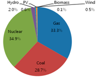
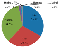
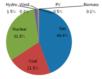
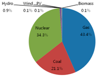
Initially, basic cost-wise optimization was performed with three costs (construction cost in Equation (2), O and M cost in Equation (3), and fuel cost in Equation (4)) and two constraints (minimal supply requirement constraint in Equation (7) and realizable potential constraint in Equation (8)). As seen in the second column of Table 1, the portion of renewable energy sources (hydro, wind, PV, and biomass) is decreasing from 4% (2.5% of hydro + 0.6% of wind + 0.8% of PV + 0.1% of biomass) initially to 3.2% in 2020 to 2.4% in 2030, with respect to generation capacity, because renewable energy sources are not cost-effective. The portion of gas sources is increasing from 31.8%, initially, to 33.3% in 2020, to 44.4% in 2030, while that of coal sources is decreasing from 36.8%, initially, to 28.7% in 2020, to 21.5% in 2030, and that of nuclear sources is fluctuating from 27.4%, initially, to 34.9% in 2020, to 31.8% in 2030.

Table 7. Optimized generation capacity (MW) from the basic model.

Year	Gas	Coal	Nuclear	Hydro	Wind	PV	Biomass	Total
2012	4372	0	1310	0	0	0	0	5682
2013	0	0	350	0	0	0	0	350
2014	0	0	1515	0	0	0	0	1515
2015	0	0	1774	0	0	0	0	1774
2016	239	0	1605	0	0	0	0	1844
2017	592	0	1316	0	0	0	0	1908
2018	667	0	1315	0	0	0	0	1982
2019	724	0	1316	0	0	0	0	2040
2020	775	0	1316	0	0	0	0	2091
2021	1205	0	1349	0	0	0	0	2554
2022	1283	0	1349	0	0	0	0	2632
2023	1363	0	1350	0	0	0	0	2713
2024	1447	0	1349	0	0	0	0	2796
2025	1532	0	1349	0	0	0	0	2881
2026	3015	0	0	0	0	0	0	3015
2027	3105	0	0	0	0	0	0	3105
2028	3199	0	0	0	0	0	0	3199
2029	3297	0	0	0	0	0	0	3297
2030	3393	0	0	0	0	0	0	3393

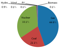
shows the optimized generation capacity from this basic model. As seen in Table 7, there is no additional capacity installation from any renewable source. Additionally, there is no additional capacity installation from coal sources because it has higher construction and fuel costs over gas sources, as presented in Table 3. Table 2 shows a similar energy mix trend with respect to the generation amount.

In order to consider carbon emission problems, the CO₂ cost in Equation (5) was also added to the above basic model. As seen in the third columns of Table 1 and Table 2, the energy mix trends from this basic + CO₂ model are similar to those of the basic model because the CO₂ cost does not contribute much when compared with the construction cost.

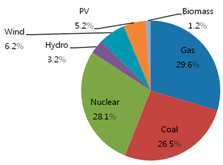
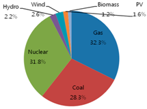
Thus, in order to more actively consider carbon emission problems, the RPS constraint in Equation (9) and PV RPS constraint in Equation (10) were added to the above basic + CO₂ model. As seen in the fourth column of Table 2, the portion of renewable energy sources from this basic + CO₂ + RPS model is increasing from 2.1%, initially, to 7.6% in 2020, to 13.0% in 2030, with respect to the generation amount because of the RPS constraint. Table 6 shows a more detailed result about the generation amount of each energy source and total renewable percentage of each year, which satisfies the RPS constraint in Equation (9). Table 1 shows similar trend of renewable energy portion with respect to generation capacity (4%, initially, to 15.8% in 2020, to 27.3% in 2030).

For this basic + CO₂ + RPS model optimization, the initial values of solution vector $I_t^e$ were set to all zeros. However, this initial solution vector with zeros could not easily find any feasible solution vector. Thus, this study used a more elaborate initial vector. For the starting values of renewable source installed capacity $I_t^{e_3}$, yearly maximum values, instead of zero, were used. For example, if realizable potential in 2012 is 1868 MW and that in 2013 is 2018 MW, the starting value of installed capacity in 2013 becomes 150 MW. 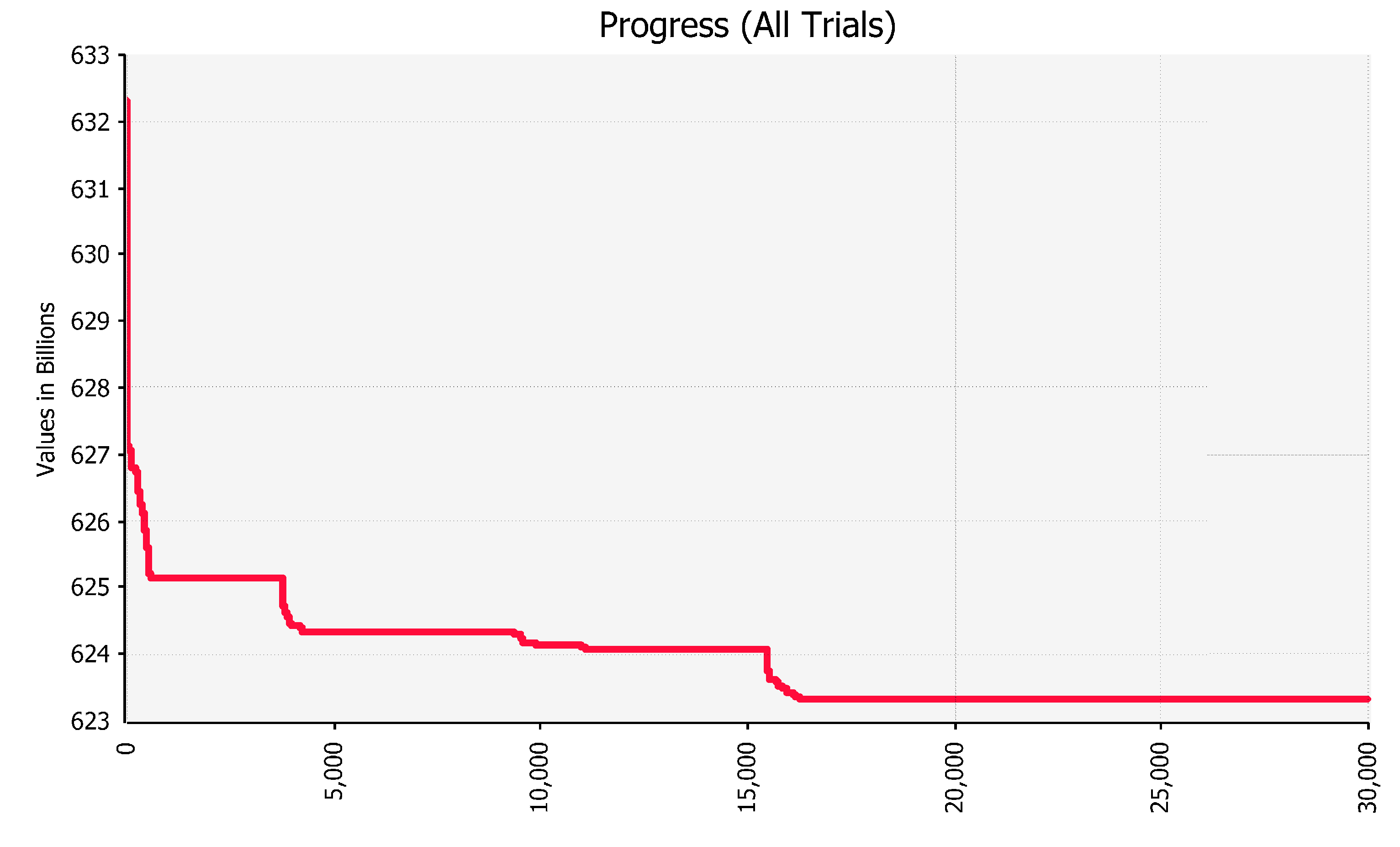Using this improved initial vector, the basic + CO₂ + RPS model could easily find the optimal solution of $623 billion, which consists of $118 billion from construction cost, $66 billion from O and M cost, $370 billion from fuel cost, and $70 billion from CO₂ cost. Figure 1 shows the convergence trend of this optimization computation.

Table 8. Optimized generation capacity (MW) from basic + CO₂ + RPS model.

Year	Gas	Coal	Nuclear	Hydro	Wind	PV	Biomass	Total
2012	6310	0	0	96	369	438	180	7393
2013	0	0	2225	0	0	401	180	2806
2014	0	0	0	230	0	0	0	230
2015	0	0	0	243	413	578	0	1234
2016	0	0	453	197	1059	814	169	2692
2017	0	0	4915	159	427	698	217	6415
2018	0	0	0	0	0	109	76	184
2019	0	0	0	254	1683	0	0	1937
2020	0	0	373	185	1562	1298	215	3632
2021	3262	0	0	69	1218	1380	189	6118
2022	0	0	6303	20	880	1297	120	8619
2023	0	0	0	74	0	0	356	430
2024	0	0	0	90	1888	1121	0	3100
2025	0	0	0	90	1,536	1072	184	2883
2026	0	0	5460	16	729	1623	216	8045
2027	0	0	0	5	252	1760	163	2179
2028	0	0	685	25	1,190	565	90	2555
2029	0	0	2659	15	332	1538	125	4668
2030	62	0	2139	15	758	1601	149	4724

shows annually installed capacity of each energy source from the basic + CO₂ + RPS model. As seen in the table, there is no additional capacity installation from coal sources, while there are only three installations (6310 MW in 2012, 3262 MW in 2021, and 62 MW in 2030) from gas sources.

The results from the basic + CO₂ + RPS model also satisfy all the constraints.

Table 9. Minimal supply requirement result from basic + CO₂ + RPS model.

Year	Generation (MWh)	Net Supply (MWh)	Demand (MWh)	Reserved (MWh)
2012	563,263	531,381	476,018	523,620
2013	582,993	549,993	478,385	526,224
2014	584,060	551,000	488,630	537,493
2015	587,645	554,383	500,622	550,684
2016	598,202	564,342	513,038	564,342
2017	642,026	605,685	525,808	578,389
2018	642,814	606,429	539,060	592,966
2019	648,857	612,129	552,689	607,958
2020	661,576	624,128	566,655	623,321
2021	694,671	655,350	583,651	642,016
2022	750,708	708,215	601,160	661,276
2023	753,641	710,982	619,195	681,115
2024	761,972	718,842	637,774	701,551
2025	770,519	726,905	656,911	722,602
2026	820,875	774,410	676,616	744,278
2027	826,665	779,873	696,910	766,601
2028	837,509	790,103	717,817	789,599
2029	863,777	814,884	739,369	813,306
2030	887,963	837,701	761,546	837,701

shows the results of the minimal supply requirement constraint. The second column of the table represents the total generation amount in each year and the third column represents the net supply amount, which is calculated by dividing the second column by $\left(1+k\right)$. The fourth column represents the demand amount and the fifth column represents the reserve-included demand, which is calculated by multiplying the fourth column and $\mathsf{\psi }$. Thus, the third column should be greater or equal to the fifth column in this constraint, and results show that this constraint is satisfied.

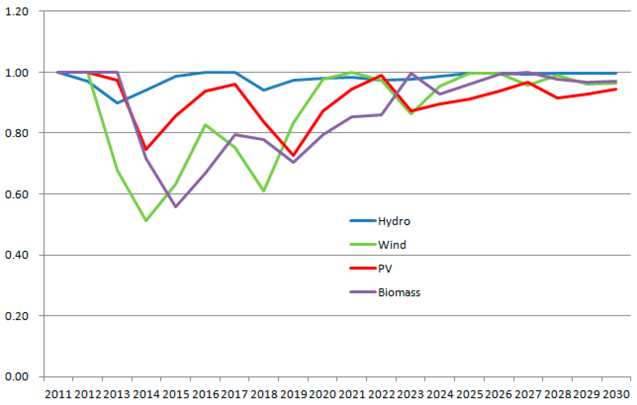
For the realizable potential constraint, the results satisfy each year’s maximal installation limits as shown in Figure 2. As seen in the figure, the hydro source minimally fluctuates near the maximal installation line, while the wind source maximally fluctuates beneath the line.

The RPS constraint was already mentioned that it was met as observed in Table 6, and for the PV RPS constraint, the PV generation amounts from 2012 to 2017 are much greater than PV RPS, as shown in Table 6.

4. Conclusions and Policy Implications

This study proposed an optimal energy mix model for electricity generation in Korea up to 2030. The results showed that from the original energy mix of 32.4% of gas, 36.6% of coal, 28.9% of nuclear, and 2.1% of renewables in 2011, the mix will become 32.3% of gas, 28.3 of coal, 31.8% of nuclear, and 7.6% of renewables in 2020, and 26.9% of gas, 21.1% of coal, 39.0% of nuclear, and 13.0% of renewables in 2030. Contrary to a cost-only optimization model, the model with RPS constraint could produce more environment-friendly energy mix results.

The proposed optimization model improved the exiting optimization formulation (unit of O and M cost, position of loss factor, yearly checking constraint, misused parenthesis, etc.), used updated data (more recent RPS, scale of emission rate, etc.), and provided more explanatory computational results. At the same time, this study tried to be as concise as possible by excluding cost-reducing effects which require complicated functions and corresponding coefficient values. Additionally, this study did not consider external costs from environmental damage because its deviation is still too high among experts [4]. Otherwise, the nuclear portion in the energy mix could be less than current results, which can be a good future research topic.

Furthermore, future study should include more realistic formulation (age structure, scraping factor, etc.), and more up-to-date data (for example, more accurate data from the seventh electricity demand and supply plan and national greenhouse gas reduction targets, and more realistic cost data). This optimization model for nation-wide energy mix planning can be applicable not only to Korea, but also to any country as long as proper data can be collected. Thus, it is expected to see more application of this energy mix model to many other countries in the future for better planning their electricity generation, while including more green energies.

References

1. EIA (U.S. Energy Information Administration). International Energy Data and Analysis. U.S. Energy Information Administration. 2014. Available online: http://www.eia.gov (accessed on 20 January 2016). [Google Scholar]
2. Eom, J.E.; Schipper, L. Trends in passenger transport energy use in Korea. Energy Policy 2010, 38, 3598–3607. [Google Scholar] [CrossRef]
3. Ku, S.J.; Yoo, S.H. Willingness to pay for renewable energy investment in Korea: A choice experiment study. Renew. Sustain. Energy Rev. 2010, 14, 2196–2201. [Google Scholar] [CrossRef]
4. Ahn, J.; Woo, J.R.; Lee, J. Optimal allocation of energy sources for sustainable development in Korea: Focus on the electric power generation industry. Energy Policy 2015, 78, 78–90. [Google Scholar] [CrossRef]
5. Park, S.Y.; Yun, B.-Y.; Yun, C.Y.; Lee, D.H.; Choi, D.G. An analysis of the optimum renewable energy portfolio using the bottom-up model: Focusing on the electricity generation sector in Korea. Renew. Sustain. Energy Rev. 2016, 53, 319–329. [Google Scholar] [CrossRef]
6. Anderson, D. Models for determining least-cost investments in electricity supply. Bell J. Econ. Manag. Sci. 1972, 3, 267–299. [Google Scholar] [CrossRef]
7. Johnston, J.; Mileva, A.; Nelson, J.H.; Kammen, D.M. SWITCH-WECC: Data, Assumptions, and Model Formulation; University of California: Berkeley, CA, USA, 2013. [Google Scholar]
8. Mai, T.; Drury, E.; Eurek, K.; Bodington, N.; Lopez, A.; Perry, A. Resource Planning Model: An Integrated Resource Planning and Dispatch Tool for Regional Electric Systems; Technical Report NREL/TP-6A20-56723; National Renewable Energy Laboratory: Golden, CO, USA, 2013. [Google Scholar]
9. Mai, T.; Barrows, C.; Lopez, A.; Hale, E.; Dyson, M.; Eurek, K. Implications of Model Structure and Detail for Utility Planning: Scenario Case Studies Using the Resource Planning Model; Technical Report NREL/TP-6A20-63972; National Renewable Energy Laboratory: Golden, CO, USA, 2015. [Google Scholar]
10. Hirth, L. The European Electricity Market Model EMMA. Available online: https://www.pik-potsdam.de/members/hirth/emma (accessed on 5 April 2016).
11. Masse, P.; Gibrat, R. Application of linear programming to investments in the electric power industry. Manag. Sci. 1957, 3, 149–166. [Google Scholar] [CrossRef]
12. Haller, M.; Ludig, S.; Bauer, N. Bridging the scales: A conceptual model for coordinated expansion of renewable power generation, transmission and storage. Renewable and Sustainable Energy Reviews 2012, 16, 2687–2695. [Google Scholar] [CrossRef]
13. Batlle, C.; Rodilla, P. An enhanced screening curves method for considering thermal cycling operation costs in generation expansion planning. IEEE Trans. Power Syst. 2013, 28, 3683–3691. [Google Scholar] [CrossRef]
14. Palmintier, B.; Webster, M. Impact of unit commitment constraints on generation expansion planning with renewables. In Proceedings of the IEEE Power and Energy Society General Meeting, Detroit, MI, USA, 24–29 July 2011.
15. Palmintier, B. Incorporating Operational Flexibility into Electric Generation Planning: Impacts and Methods for System Design and Policy Analysis. Ph.D. Thesis, Massachusetts Institute of Technology, Cambridge, MA, USA, February 2013. [Google Scholar]
16. De Sisternes, F.J. Investment Model for Renewable Electricity Systems (IMRES): An Electricity Generation Capacity Expansion Formulation with Unit Commitment Constraints; Working Paper 2013-016; MIT Center for Energy and Environmental Policy Research (CEEEPR): Cambridge, MA, USA, 2013. [Google Scholar]
17. Stoll, H.G. Least-Cost Electric Utility Planning; John Wiley and Sons: New York, NY, USA, 1989. [Google Scholar]
18. Schweppe, F.C.; Merrill, H.M.; Burke, W.J. Least-cost planning: Issues and methods. Proc. IEEE 1989, 77, 899–907. [Google Scholar] [CrossRef]
19. Hirst, E.; Schweitzer, M. Electric utility resource planning and decision making: The importance of uncertainty. Risk Anal. 1990, 10, 137–146. [Google Scholar] [CrossRef]
20. Hobbs, B.F. Optimization methods for electric utility resource planning. Eur. J. Oper. Res. 1995, 83, 1–20. [Google Scholar] [CrossRef]
21. Bhattacharya, A.; Kojima, S. Power sector investment risk and renewable energy: A Japanese case study using portfolio risk optimization method. Energy Policy 2012, 40, 69–80. [Google Scholar] [CrossRef]
22. Mendes, C.; Soares, I. Renewable energies impacting the optimal generation mix: The case of the Iberian Electricity Market. Energy 2014, 69, 23–33. [Google Scholar] [CrossRef]
23. Vidal-Amaro, J.J.; Østergaard, P.A.; Sheinbaum-Pardo, C. Optimal energy mix for transitioning from fossil fuels to renewable energy sources—The case of the Mexican electricity system. Appl. Energy 2015, 150, 80–96. [Google Scholar] [CrossRef]
24. Turvey, R.; Anderson, D. Electricity Economics: Essays and Case Studies; The Johns Hopkins University Press: Baltimore, MA, USA, 1977. [Google Scholar]
25. Mays, L.W.; Tung, Y.K. Hydrosystems Engineering and Management; McGraw-Hill: New York, NY, USA, 1992. [Google Scholar]
26. IEA (International Energy Agency). Projected Costs of Generating Electricity; International Energy Agency: Paris, France, 2010. [Google Scholar]
27. KEPCO (Korea Electric Power Corporation). Financial Effect Analysis and Counterplan Establishment of RPS; Korea Electric Power Corporation: Seoul, Korea, 2010. [Google Scholar]
28. EIA (U.S. Energy Information Administration). Annual Energy Outlook 2012; U.S. Energy Information Administration: Washington, DC, USA, 2012.
29. EPSIS (Korea Electric Power Statistics Information System). EPSIS. 2012. Available online: http://epsis.kpx.or.kr (accessed on 20 January 2016).
30. Kim, S.; Koo, J.; Lee, C.J.; Yoon, E.S. Optimization of Korean energy planning for sustainability considering uncertainties in learning rates and external factors. Energy 2012, 44, 126–134. [Google Scholar] [CrossRef]
31. KEMCO (Korea Energy Management Corporation). Renewable Energy Whitepaper; Korea Energy Management Corporation: Seoul, Korea, 2010. [Google Scholar]
32. KEMCO (Korea Energy Management Corporation). Renewable Portfolio Standard Guidebook; Korea Energy Management Corporation: Seoul, Korea, 2012. [Google Scholar]
33. Evolver, Palisade Corporation. Ithaca, NY, USA, 2016.
34. Geem, Z.W.; Hong, J. Improved formulation for the optimization of wind turbine placement in a wind farm. Math. Probl. Eng. 2013, 2013. Aritcle 481364. [Google Scholar] [CrossRef]
35. Kim, J.; Geem, Z.W. Optimal scheduling for maintenance period of generating units using a hybrid scatter-genetic algorithm. IET Gener. Transm. Distrib. 2015, 9, 22–30. [Google Scholar] [CrossRef]
Figure 1. Convergence history of energy mix optimization in Korea.
Sustainability 08 00423 g001
Figure 2. Optimal generation capacity versus realizable potential in each year.
Sustainability 08 00423 g002