Dynamic EROI Assessment of the IPCC 21st Century Electricity Production Scenario

Abstract

The Energy Return on Investment (EROI) is an important measure of the energy gain of an electrical power generating facility that is typically evaluated based on the life cycle energy balance of a single facility. The EROI concept can be extended to cover a collection of facilities that comprise a complete power system and used to assess the expansion and evolution of a power system as it transitions from one portfolio mix of technologies to another over time. In this study we develop a dynamic EROI model that simulates the evolution of a power system and we perform an EROI simulation of one of the electricity production scenarios developed under the auspices of the Intergovernmental Panel on Climate Change (IPCC) covering the global supply of electricity in the 21st century. Our analytic tool provides the means for evaluation of dynamic EROI based on arbitrary time-dependent demand scenarios by modeling the required expansion of power generation, including the plowback needed for new construction and to replace facilities as they are retired. The results provide insight into the level of installed and delivered power, above and beyond basic consumer demand, that is required to support construction during expansion, as well as the supplementary power that may be required if plowback constraints are imposed. In addition, sensitivity to EROI parameters, and the impact of energy storage efficiency are addressed.

1. Introduction

1.1. Background

The Intergovernmental Panel on Climate Change (IPCC) scenarios that describe the portfolio mix of global electricity sources for the 21st century are characterized by a transition from carbon-based fossil fuels to renewables that implies a dramatic expansion in particular of solar and wind power. These sources are different than traditional ones in terms of their Energy Return on Investment (EROI) and the timing of energy investment over their life cycle (nearly all input energy goes to construction and very little during operation). In addition, other factors such as the need for energy storage tend to reduce overall EROI. Our study aims to address these concerns and identify possible risks associated with the planned expansion. In the prior development of the dynamic EROI concept by Kessides and Wade [1] the focus was on a closed-form solution for energy payback time and energy doubling of a power system with fixed plowback fraction. In the present work we extend this concept to accommodate arbitrary time-dependent demand scenarios in order to determine the required expansion of power generation, including the plowback needed for new construction and to replace facilities as they are retired. Since it is very difficult to generalize the EROI parameters, especially the input energy requirement, we look at a range of values to examine sensitivity.

1.2. EROI Definitions

The definition of EROI used herein is described by the following equations.

$$EROI=\frac{E_{output}}{E_{input}}$$

(1)

The numerator E_output, is the gross electrical energy produced over the lifetime of a power generating facility and the denominator, E_input, is the energy invested to fabricate, construct and operate the facility over its lifetime. Since some of the invested input energy may not be in the form of electricity it is necessary to express all input and output energy quantities on the basis of their primary thermal equivalents. Calculation of E_output is relatively straightforward using basic, readily available parameters.

$$E_{output}=\frac{P_r{f}_d{T}_L}{\eta }$$

(2)

where

• P_r(t) is the total rated nameplate capacity
• f_d is the duty cycle (capacity factor)
• T_L is the individual plant lifetime
• η is the efficiency of conversion from primary thermal power to electrical power that is characteristic of the host electrical grid, which we assume equal to 0.333

Calculation of E_input is complicated by the need for a Life Cycle Analysis (LCA) that considers the entire energy supply chain involved in constructing a power generating facility, providing the fuel resource, operating the facility, and decommissioning the facility. Note that, in cases where a fuel (e.g., gas, coal, uranium, etc.) is involved the energy content of the fuel itself is not included, only the energy required to mine, process, and deliver it is included.

An additional complexity arises when the various energy input sources (e.g., for manufacturing components, mining fuel, etc.) are summed. To capture the full input energy in a consistent manner it is necessary to consider the conversion efficiency involved in producing secondary input energy sources such as electricity, and to sum over the primary thermal equivalent energies of all input sources. Electrical input energy must always be included based on its thermal equivalent based on an assumed thermal-to-electrical conversion efficiency.

In our analysis we consider the production of electrical energy by various types of sources and, for each type of source, divert a fraction of the gross electrical output energy toward the operation of existing sources and construction of new ones of the same type. In reality, input electrical energy to, say, manufacture solar panels would be derived from the full portfolio of generators on the grid but in the present work we require that the capacity expansion of each type of source be self-sufficient (to the extent that it can, within limits) in terms of input energy.

Moreover, for any type of source, whether or not the various needs for input energy (manufacturing, mining, transportation, etc.) would in practice be met using electricity or not, we plow back the electrical energy and factor in the conversion efficiency such that input needs are supplied by that source on a primary thermal equivalent basis as follows.

$$E_{input}=E_{cd}+\frac{P_r{f}_d{f}_o{T}_L}{\eta }$$

(3)

where

• E_cd is the primary thermal equivalent energy for construction and decommissioning
• f_o is the fraction of generated electrical power for operation and maintenance

2. Materials and Methods

2.1. Modeling

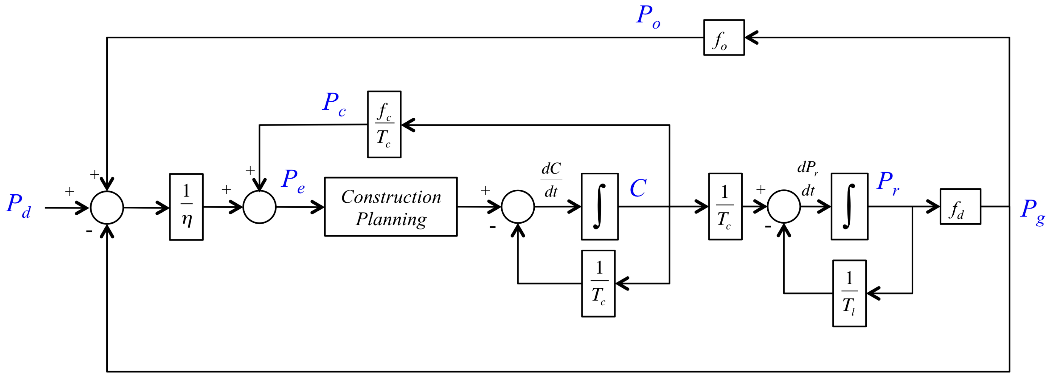
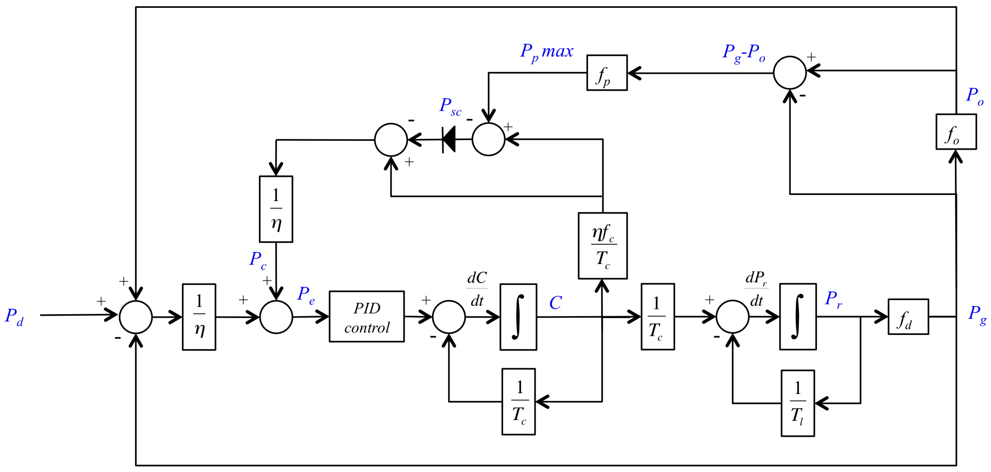
2.1.1. Simulation Model

Again, following [1], except using a different variable name convention, modeling is based on two coupled first order differential equations, one covering the mobilization of construction activities, the other covering the construction of new units and the retirement of old units.

$$\frac{d}{dt}{P}_r(t)=-\frac{1}{T_L}{P}_r(t)+\frac{C(t)}{T_c}$$

(4)

$$\frac{d}{dt}C(t)=\frac{(1-f_o)f_d{f}_p{P}_r(t)}{f_c}-\frac{C(t)}{T_c}$$

(5)

where

• P_r(t) is the total rated nameplate capacity
• T_L is the individual plant lifetime
• T_c is the individual plant construction time
• C(t) is the nameplate rated generating capacity under construction
• f_o is the fraction of generated power required for operations and maintenance
• f_d is the duty cycle (capacity factor)
• f_p is the fraction of generated power that is plowed back to construct new plants
• f_c is the primary thermal equivalent energy for construction per unit of nameplate rating

In this treatment we make the approximation that the energy required for decommissioning is negligible compared to that for construction so that f_c is derived from E_cd but is used to determine output energy diverted to construction (only).

A block diagram representation is given in Figure 1, where P_d is the electrical demand, P_g is the generated electrical power, P_o is the electrical power used for operation and maintenance, P_c is the “plowback power” used for construction, and P_e is the imbalance (error) power. Note that P_c and P_e are expressed in terms of their thermal equivalents. A “construction planning” process is applied to the error to stimulate new construction.

We developed a construction planning scheme as incorporated in Figure 2. Here we use the plowback fraction f_p to enforce a limit on plowback power P_p, and introduce supplemental power P_s when necessary to achieve the desired level of construction power P_c. The supplemental power would come from some other source, and the collection of plants being modeled would only supply the plowback power P_{p_max}. This allows for the simulation of situations where another source is “cannibalized” to provide the energy necessary to deploy the source in question. We deploy a proportional-integral-derivative (PID) controller with settings chosen to minimize sum of squares error over the period of simulation.

2.1.2. Simulation Input Data

We considered coil, gas, nuclear, solar, wind, and hydro sources of electricity. We examined EROI, Energy Payback Time (EPBT), and LCA data from numerous published sources over the range of power generating technologies and converged on those sources which provided enough detail so that we could understand the technological basis, and separate the energy inputs into categories of construction, decommissioning, operations, and fuel processing. Then, for each power generating technology, we averaged the data from multiple studies after normalizing to power rating and harmonizing on capacity factor and lifetime. All energy inputs were converted to a primary thermal equivalent (PTE) basis (electricity input was multiplied by 1/η).

We note that much of the published information is based on meta-analysis that typically mixes together different technologies, capacity factors, lifetimes, etc., sometimes leading to questionable and misleading results. The approach we have taken aims to provide an equitable basis for comparison. We also note that one our references Weisbach et al. [2], is chosen in part because it covers the full range of power generating sources, separately lists each category of energy input, and indicates the fraction of each category derived from electricity. However, this reference has been subject to some criticism [3], mainly concerning issues related to EROI definitions. But the basic data concerning energy input has not been the cause for debate, and in fact we have found it to be relatively close to the findings of others, after proper harmonization.

For coal we harmonized to a 40 year lifetime and 0.55 capacity factor [4] and then averaged the input energy data from Weisbach et al. [3] for hard coal and brown coal with the results from White and Kulchinski [5]. After harmonization, the data from these sources was in relatively close agreement.

For gas we harmonized to a 40 year lifetime and 0.56 capacity factor [2] and then averaged the input energy data from Meier and Kulchinski [6] with the results from Spath and Mann [7], both of which correspond to Combined Cycle Gas Turbine (CCGT) technology. After harmonization, the data from these sources was in relatively close agreement. The data on gas from Weisbach et al. [2] differed by an order of magnitude for reasons not understood, although in that study the fuel processing energy lost to gas flaring was excluded whereas it was included in the others.

For nuclear we harmonized to a 40 year lifetime and 0.92 capacity factor [2] and then averaged the input energy data from Weisbach et al. [2], White and Kulchinski [5], Lenzen [8], and Schneider et al. [9] (fuel portion only). All included data was based on centrifuge fuel enrichment technology. This is a key point since the (now obsolete) diffusion technology has a much higher input energy and the mixing of centrifuge and diffusion technology in meta-analysis that includes old data leads to misleading results. We find that all of the cited sources are in relatively close agreement after harmonization. Note that all cases are based on “once-through” fuel processing in which case the residual energy in spent fuel is not recovered using re-processing. The possibility of advanced breeding fuel cycles that could result in more than two orders of magnitude more energy per kg of mined uranium [9] is noted but was not considered.

For solar we consider photovoltaic (PV) only. We harmonized to a 25 year lifetime and 0.17 capacity factor and then averaged the input energy data from Bhandari et al. [10]. This harmonized data set covers five different PV technologies (mono-Si, poly-Si, a-Si, CdTe, and CIGS). Since all of these are candidates for present and future use we averaged the data with equal weighting. We do note that these technologies exhibit a wide range of EPBT/EROI so that competition on this basis could lead to a preference toward the better performers (e.g., CdTe) in the future. We chose a 25 year lifetime since this is the typical manufacturer’s warranty period, at which time the performance has degraded by 20% based on a degradation rate of 0.8% per year [11]. This degradation, due to environmental exposure and aging, is not reflected in the performance data used herein. The chosen capacity factor of 0.17 (1486 kWh/m²-year) corresponds to the global average insolation across regions of land where the average incoming solar radiation exceeds 1000 kWh/m², considered to be the cut-off for economic viability [12]. The fact that this is less than the EIA value (based on U.S. average in 2015) [2] is consistent with the notion that existing installations utilize prime sites, whereas deployment on a global basis will be less optimal.

For wind we harmonized to a 25 year lifetime and 0.23 capacity factor and then averaged the input energy data from Weisbach et al. [2] and White and Kulchinski [5], both corresponding to on-shore wind technology. We assume global exploitation will be implemented at midrange of average wind speeds presently used in wind turbine design [13], corresponding to annual average of 6.5 m/s, 2000 full-load hours per year, f_d = 23%. Again, the fact that this is less than the EIA value (based on U.S. average in 2015) [2] is consistent with the notion that existing installations utilize prime sites, whereas deployment on a global basis will be less optimal.

For hydro we harmonized to a 70 year lifetime and 0.36 capacity factor [2] and adopted the input energy data from Weisbach et al. [2]. This data corresponds to a “run-of-river” plant and exhibits a lower EROI than “reservoir” plants but considering that most future exploitation will involve run-of-river, it is more relevant to the present study.

Note that the data do not factor in, for solar and wind, the energy associated with grid integration (energy storage and transmission expansion). These factors will tend to increase the input energy E_cd as required for initial deployment, and will introduce losses associated with charge and discharge of energy storage systems and long distance transmission. Some researchers [2,14] have attempted to quantify this but the lack of technologically mature, large scale electrical energy storage options is problematic so we have only considered the possible degradation due to efficiency reduction and have not included the embodied energy. Input data used in this study is given in

Table 1. Input data for dynamic Energy Return on Investment (EROI) analysis.

Parameter	Coal	Gas	Hydro	Nuclear	Solar	Wind
fd	0.55	0.56	0.36	0.92	0.17	0.23
TL (years)	40	40	70	40	25	25
Tc (years) [15]	6	6	4	6	2	3
fo (TJ_e/TJ_e)	0.022	0.117	0.000	0.010	0.007	0.003
fc (MW-year_pte/MW_e)	0.170	0.124	0.655	0.344	1.163	0.246
EROI (Tj_e/Tj_pte)	13	3	38	25	4	19
EROI (Tj_pte/Tj_pte)	40	8	115	74	11	58
EPBT_pte (months)	1.3	1.0	21.9	1.5	27.3	4.3
Construction (TJ_pte/MW_e)	5.0	3.9	20.0	6.6	35.7	7.6
Decommissioning (TJ_pte/MW_e)	0.3	0.0	0.7	4.3	0.9	0.2
Operations (MJ_pte/MW-h_e)	36	18	0	54	25	31
Fuel Processing (MJ_pte/MW-h_e)	205	1250	0	59	0	0

. All data is on a primary thermal equivalent (PTE) basis.

We do acknowledge that, for each source, a more diverse technological range will exist and will evolve over time. We also note that, as the grid transitions to renewable technologies that do not require energy conversion from thermal to electrical, the overall grid efficiency η will improve alter the EROI. We do not factor this into the present work.

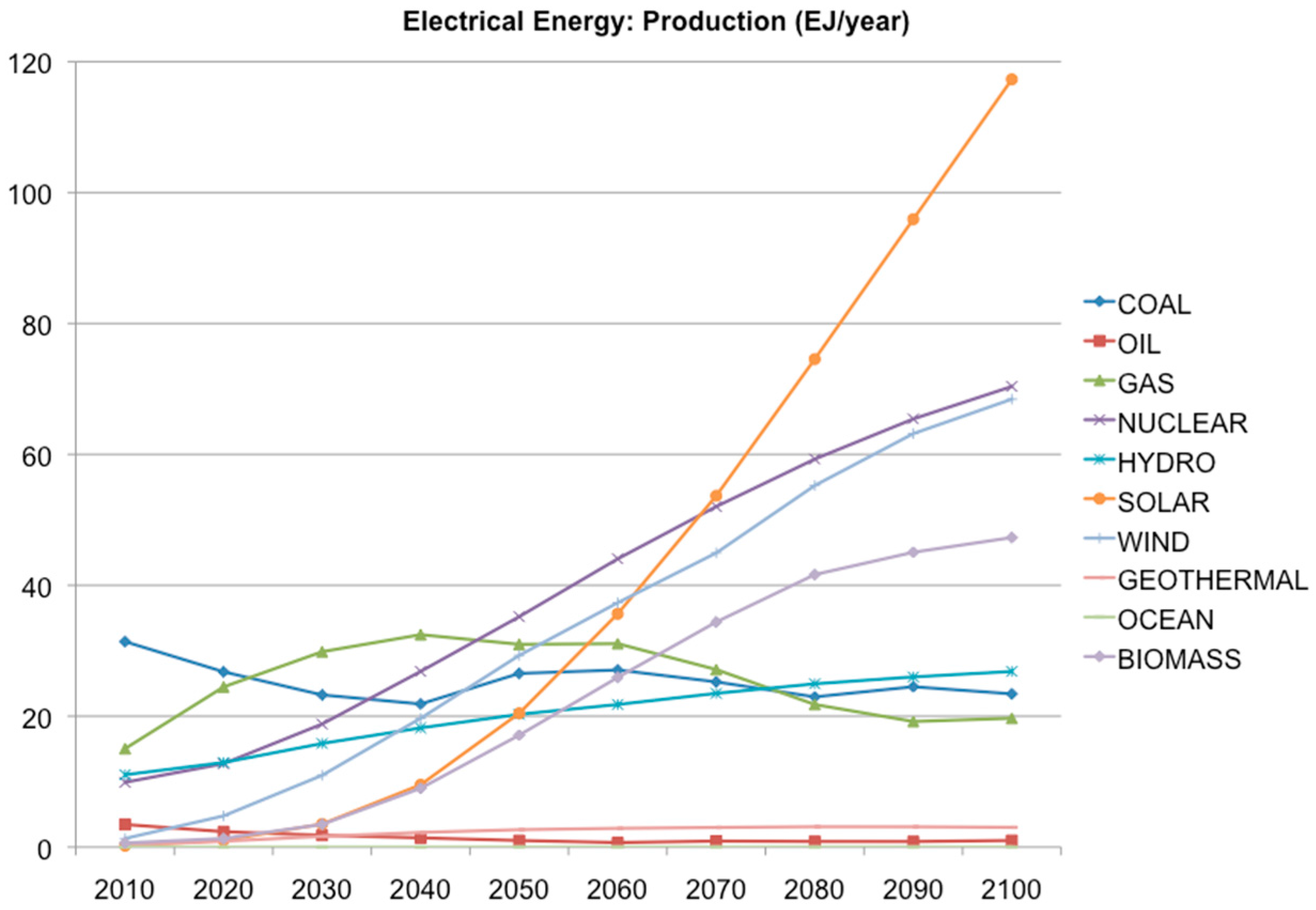
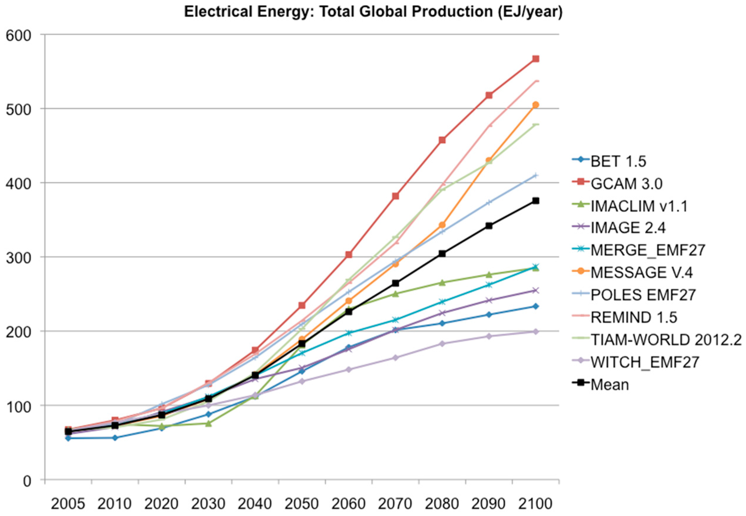
2.1.3. Simulation Scenario

The Intergovernmental Panel on Climate Change (IPCC) is evaluating means for limiting the atmospheric greenhouse gas concentration to 450 or 550 ppm CO₂ equivalent by 2100. The Fifth Assessment Report (AR5) of Working Group III of the IPCC has amassed a scenario database comprised of 31 models and 1184 scenarios. The Stanford Energy Modeling Forum Study 27 (EMF-27) is one of the sources that fed into the AR5 scenario database. We have evaluated one particular global electricity supply and consumption scenario from the AR5 database called “EMF27-450-Full_Tech” that is associated with one of the more aggressive (and successful) cases that aims to limit greenhouse gases at the end of the century at a 450 ppm CO₂ limit with mitigation using the full set of available technologies [16]. As shown in Figure 3 the AR5 database contains the results of 10 different integrated assessment models as they apply to the EMF-27 scenario. In our work we take the mean of these 10 scenarios as the basis for evaluation. The utilization of the various sources of electricity (coal, oil, gas, nuclear, hydro, solar, wind, geothermal, ocean, and biomass) is shown in Figure 4 by source, in Figure 5 by fraction of total, and in Figure 6 by production normalized to 2010 value. Several aspects of the EMF27-450-Full_Tech scenario are noteworthy:

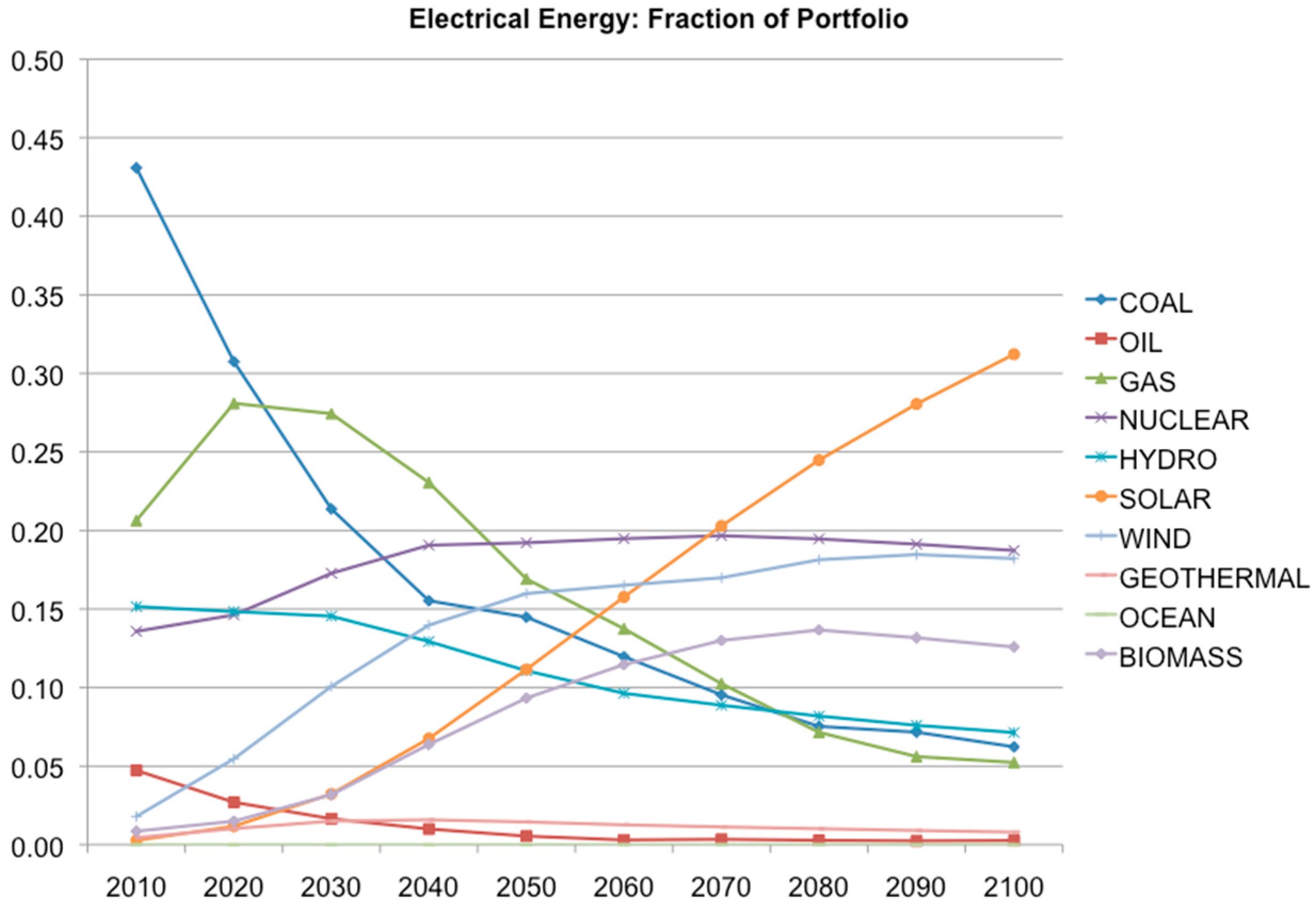
• It covers global electricity production, and the portfolio fractions may be markedly different in individual regions;
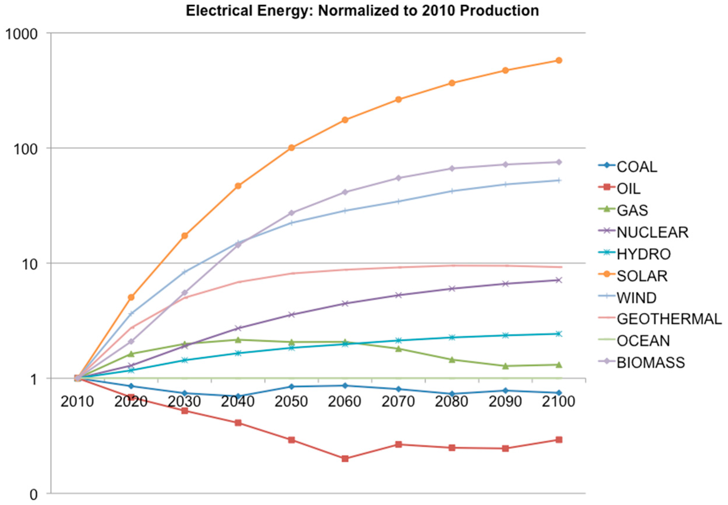
• Solar (117 EJ/year), Nuclear (70 EJ/year), Wind (68 EJ/year) and Biomass (47 EJ/year), become the dominant sources at end of century;
• Growth in solar over present levels is a prominent feature (Solar 580x, Biomass 75x, Wind 52x, Nuclear 7x);
• The fraction of intermittent sources (solar + wind) is ~50% at the end of the century on a global basis (presumably higher in some regions and lower in others but global distribution not provided with the data).

3. Results

We applied the simulation model, using the data given in Table 1, to the mean of EMF27-450-Full Tech scenario models for coal, gas, nuclear, hydro, solar, and wind. We did not analyze oil or geothermal since their portfolio fraction is small and since LCA data was not readily available. Data is linearly extrapolated between breakpoints (every 10 years, which is noted to cause some minor noise in the PID loop since the derivative is discontinuous at the breakpoints). We set a limit on plowback fraction f_pmax = 1.0, allowing, potentially, all the net output from each energy source to be used for constructing new infrastructure of the same type. Results are given in Figure 7, Figure 8, Figure 9, Figure 10, Figure 11 and Figure 12 where the power (P) and energy (E) in various categories (see following key) is plotted along with the EROI and plowback fraction f_p.

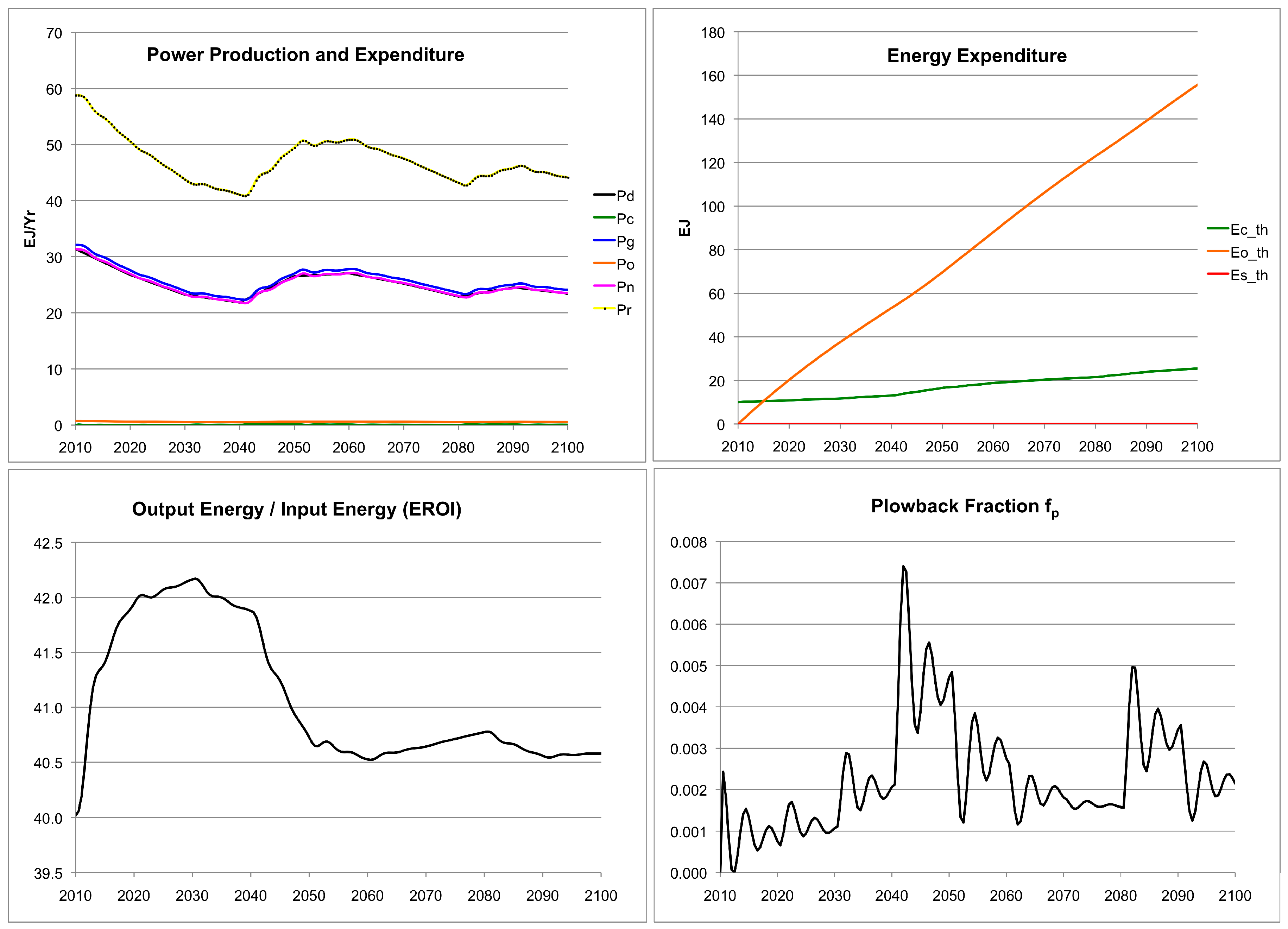
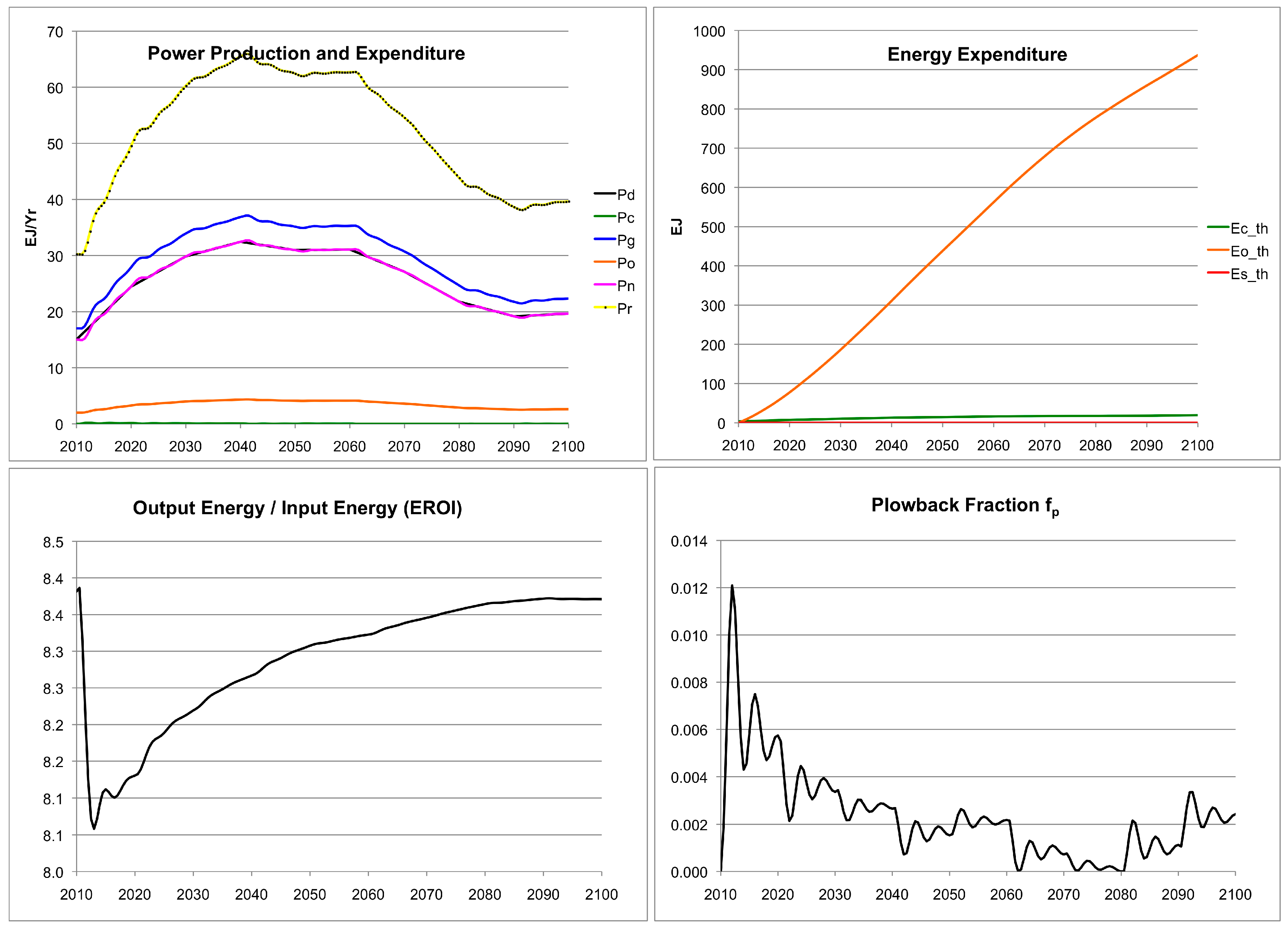
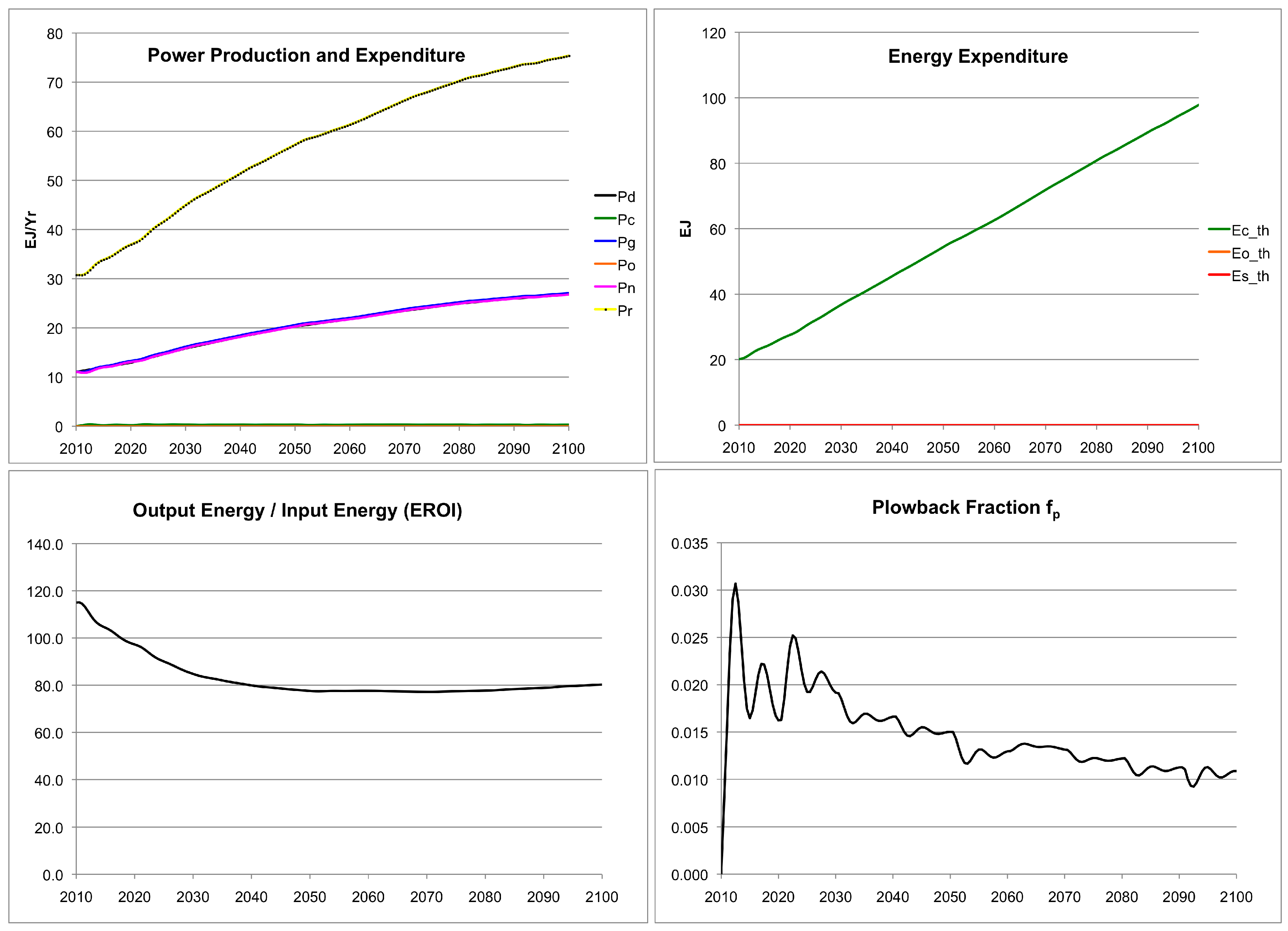
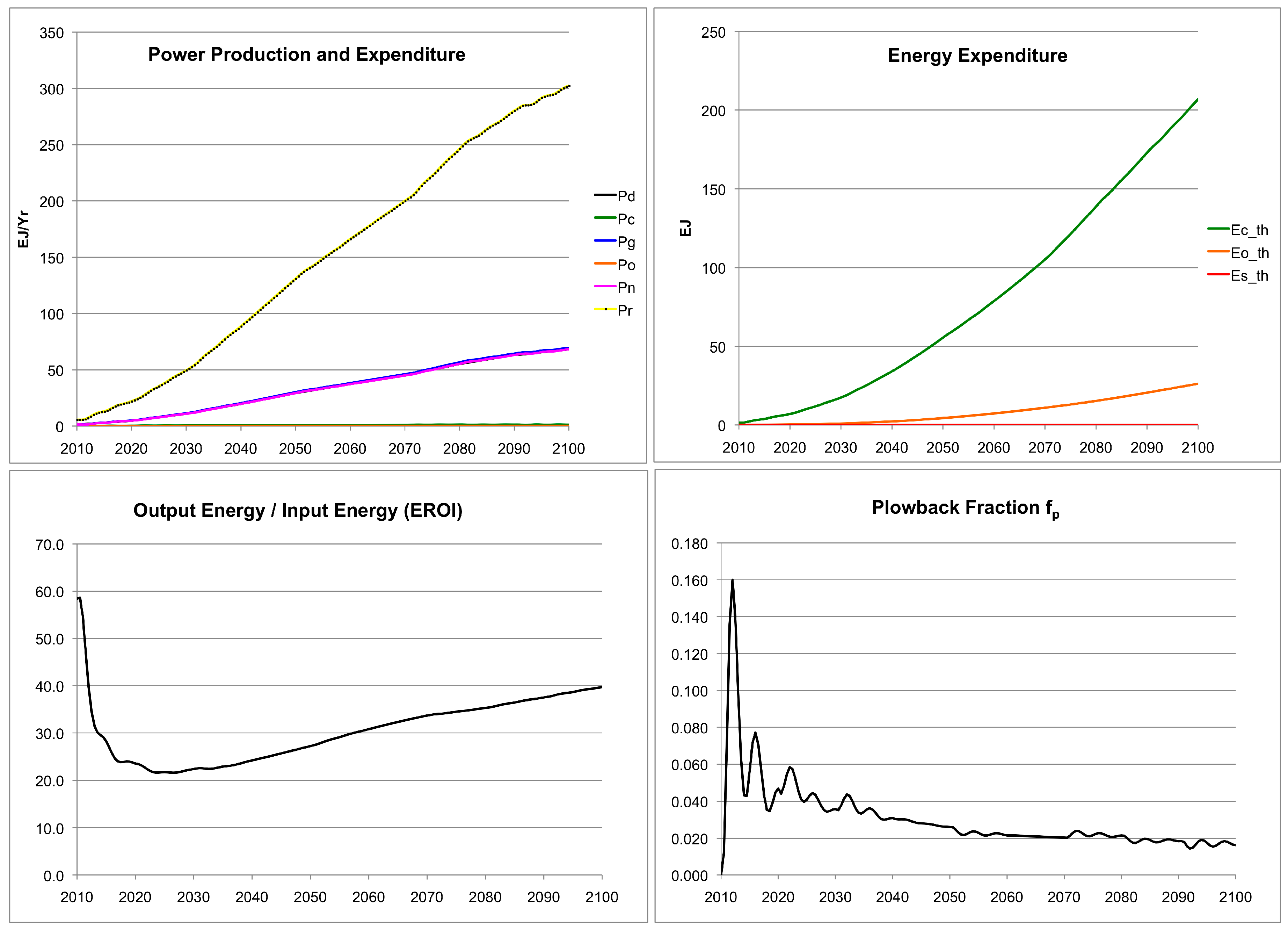
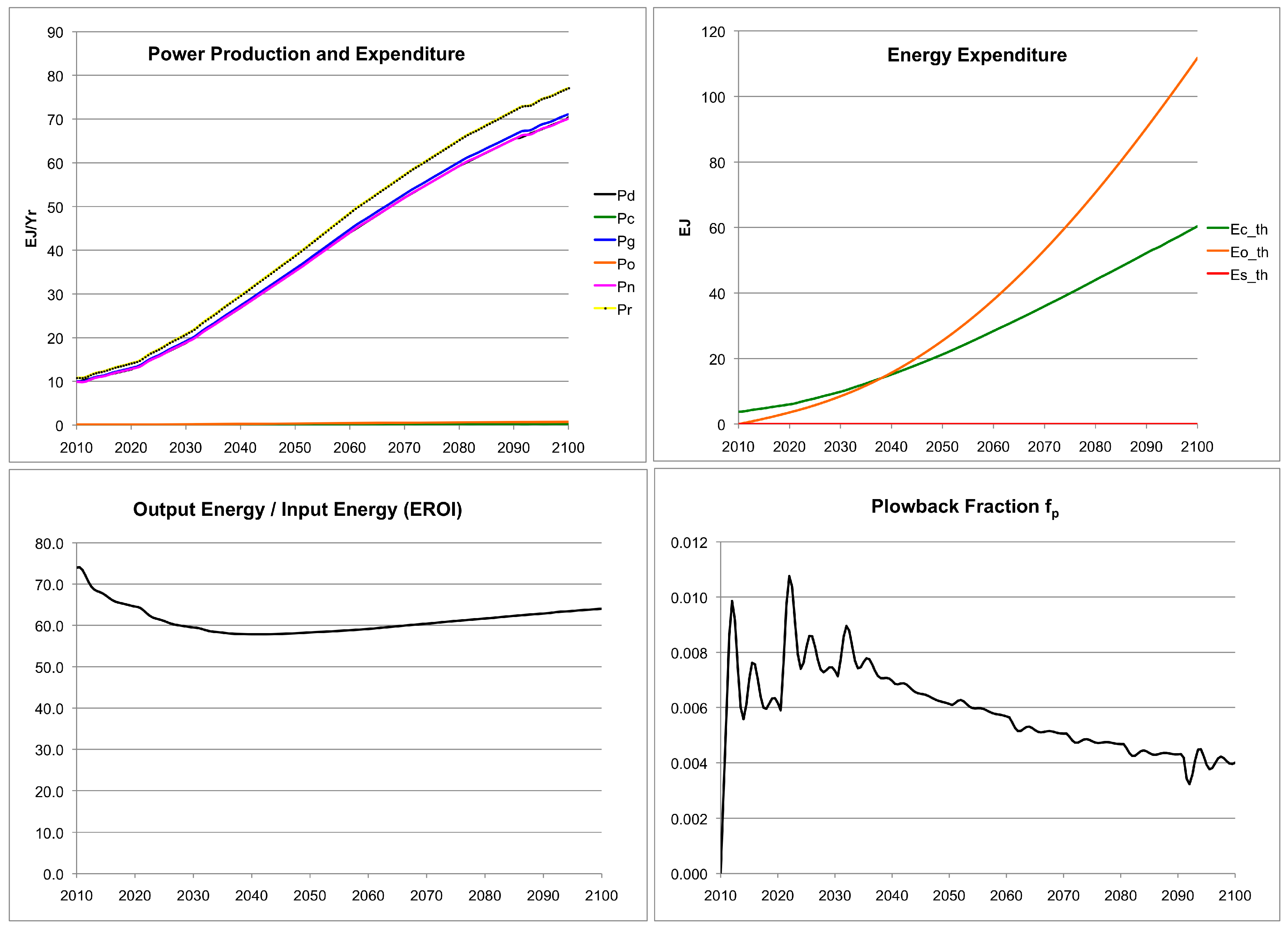
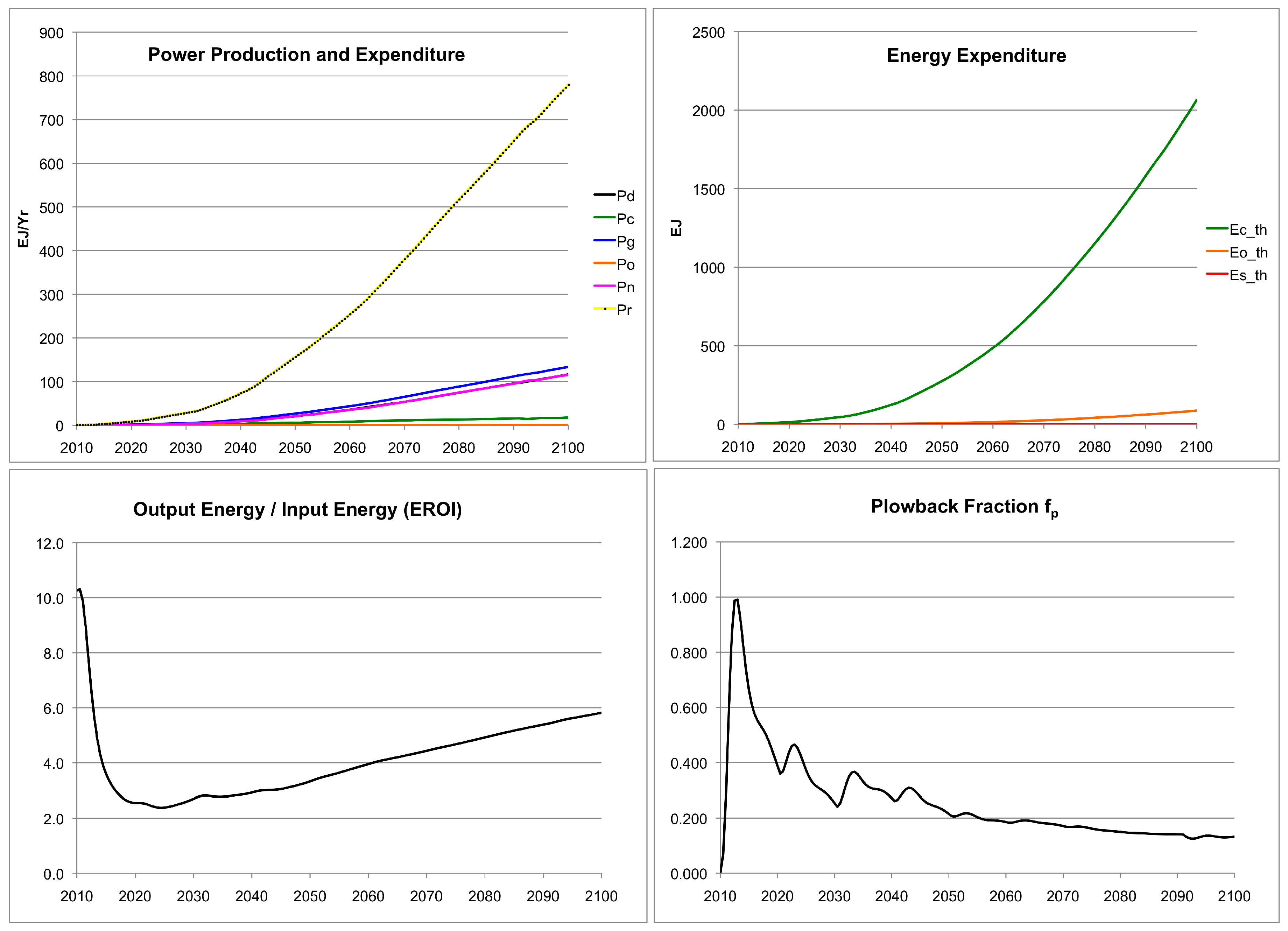
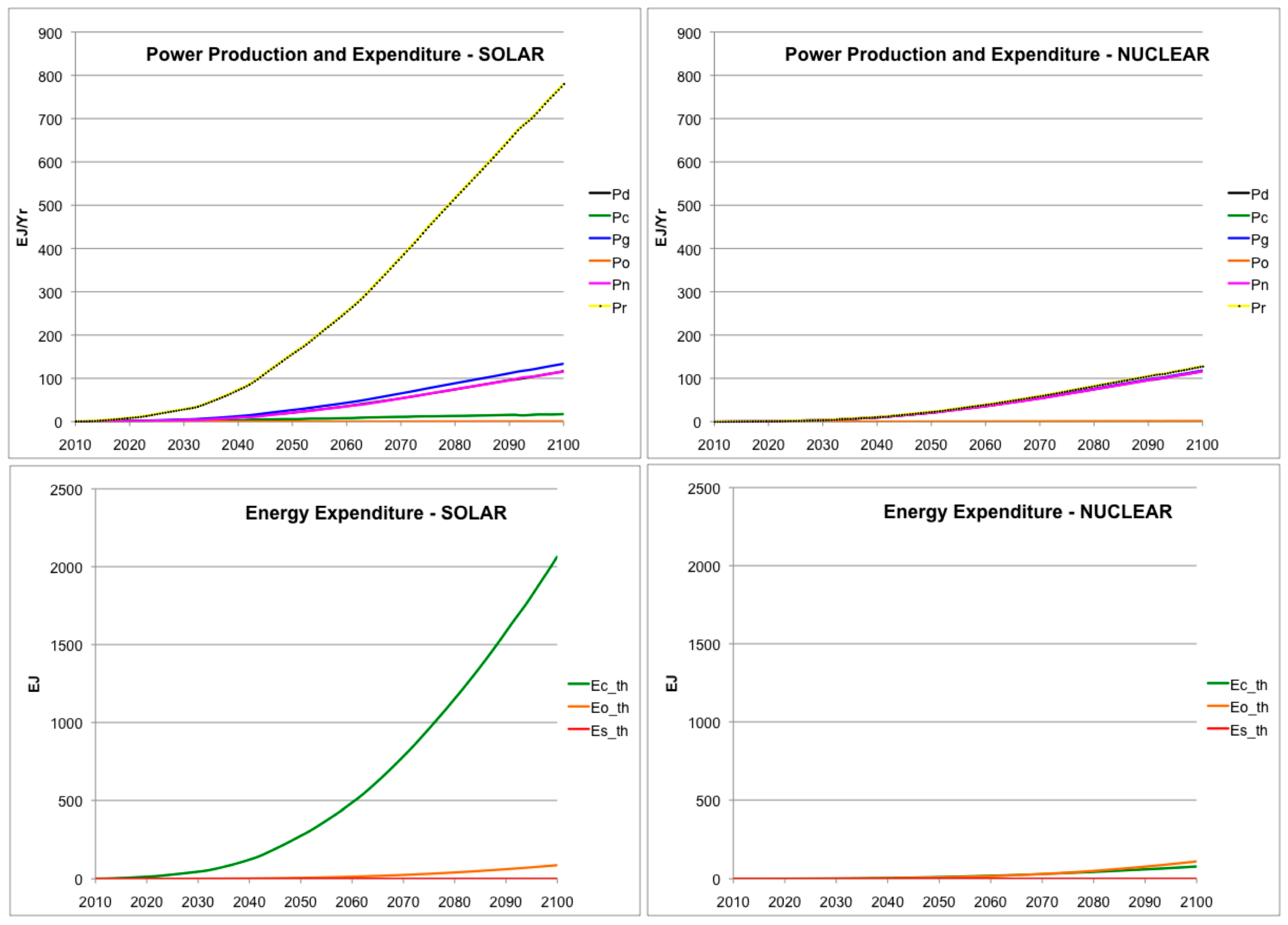
Key for variable name subscripts:

• d = demand
• c = construction
• p = plowback
• g = generated
• o = operating
• n = net (generated – operating)
• r = nameplate rated
• s = supplemental

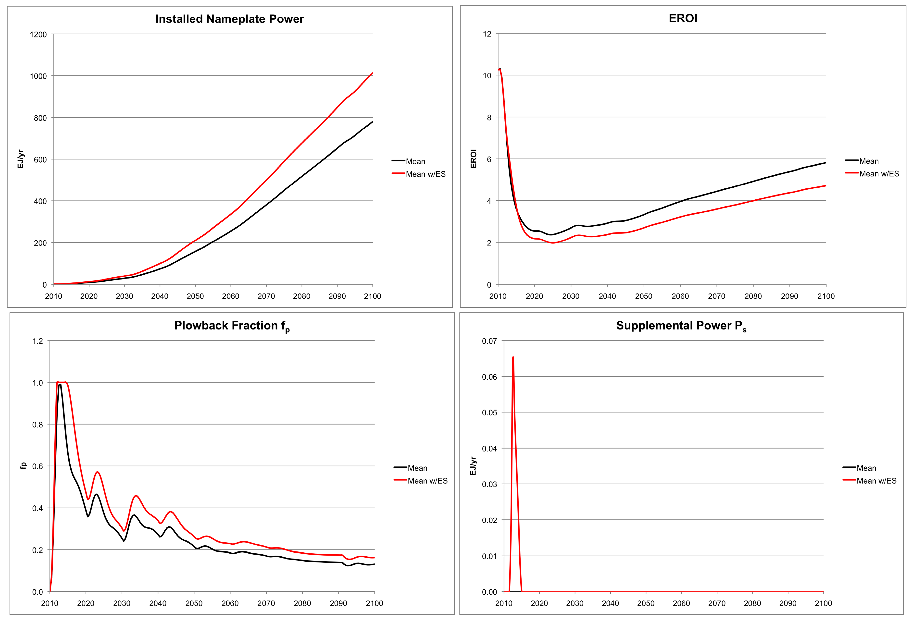
4. Discussion

The simulation results show that the plowback power and energy lead that arise from capacity expansion tend to increase the installed power requirement and diminish the EROI compared to a static situation. Sources with rapid growth exhibit the largest difference between static and dynamic EROI. Energy generated and consumed is summarized in

Table 2. Summary of electrical energy 2010–2100 (EJ PTE).

	Generated	Operations Consumption	Construction Consumption	Net to Loads	Dynamic EROI	Static EROI
Coal	6953	156	25	6771	38	40
Gas	7976	937	20	7019	8	8
Nuclear	10,747	112	60	10,574	62	74
Hydro	5535	0	98	5437	57	115
Solar	12,510	87	2066	10,358	6	11
Wind	9175	26	207	8942	39	58
Total	53,276	1326	2478	49,472	14	-

.

By the end of the century the total generated energy must exceed the energy supplied to consumers by about 8% in order to supply operations and to emplace new infrastructure. We find that solar reaches the plowback limit of 1.0 briefly during the period of initial capacity expansion. Because its portfolio fraction remains relatively constant compared to other sources that are rapidly expanding, nuclear provides the largest total energy to consumers by the end of the century.

It is informative to compare the base case of supply expansion for solar to a case where nuclear is substituted to supply solar’s share of energy delivery. A comparison, with data plotted on the same scale, is given in Figure 13. Roughly 2000 EJ more energy has to be expended to meet the demand using solar, compared to nuclear. This result highlights the difference in behavior between a traditional power source (nuclear) and a renewable (solar) under dynamic conditions of power system expansion. The traditional source has higher EROI and capacity factory, longer lifetime, and a high fraction of its input energy requirement is spread over the operating lifetime because of the fuel requirement. The renewable source has a lower EROI and capacity factory, shorter lifetime, and requires nearly all of its input energy at the beginning since it does not require fuel.

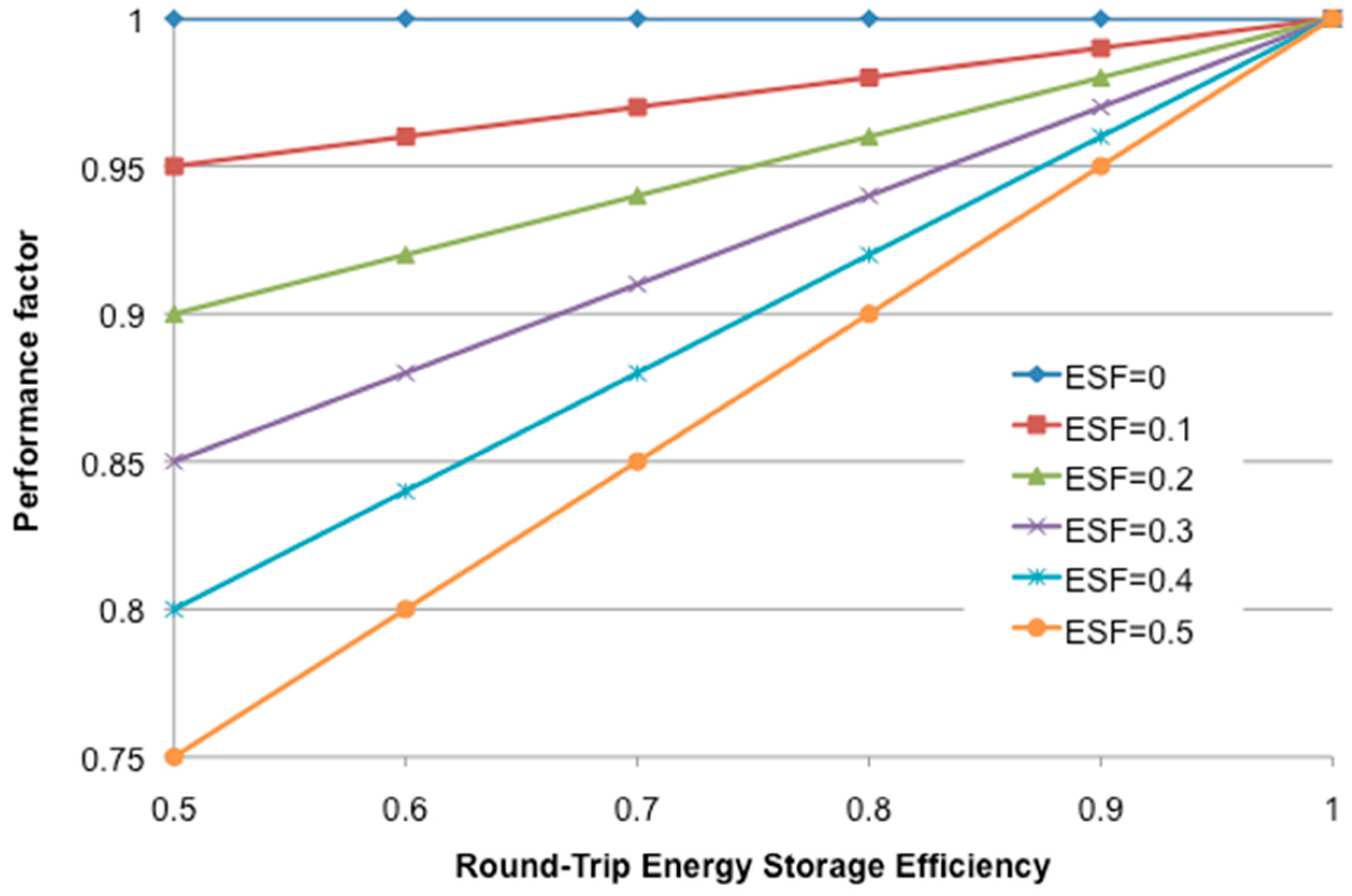
Sensitivity Analysis

We assessed sensitivity of the results with a partial accounting for grid integration. As previously mentioned the data does not include, for solar and wind, the energy associated with grid integration (energy storage and transmission expansion). These factors will tend to increase the input energy E_cd for initial infrastructure deployment, and will reduce operating efficiency due to the charge and discharge of energy storage systems. To investigate this effect, partially at least, it is easy to factor in the losses based on the round-trip efficiency η_ES of the energy storage system and the fraction f_ES of generated energy that is stored before delivery as shown in Figure 14.

$$f=1-f_{ES}\left(1-{\eta }_{ES}\right)$$

(6)

To bracket the effect, we adopt a factor of 0.8, based on η_ES = 60% efficiency and f_ES = 50% storage. To investigate the sensitivity we ran the simulation for solar with a range of EROI values from Table 1 with, and without, the performance degradation due to energy storage.

Results for solar are given in Figure 15 with and without inclusion of losses due to energy storage. Note that these results do not present the complete picture because the energy required to emplace the energy storage and transmission infrastructure is not factored in. Note that as the performance degrades with the inclusion of energy storage, more supplementary power is required to cover the demand when the plowback limit is reached.

5. Conclusions

Our results, based on the Kessides and Wade [1] dynamic EROI model, extend the assessment of power system expansion by allowing an arbitrary, time dependent demand scenario. We then collected the best available EROI data over the range of power sources and applied the model to a set of scenarios developed by the Stanford EMF-27 group for the global supply of electricity through the remainder of the 21st century.

We find that:

• The energy required to emplace and operate the infrastructure can be significant, especially at high rates of expansion, and has not been included explicitly in the overall IPCC scenario assessment;
• Due to significant uncertainty in the input energy (the denominator of the EROI ratio), there is a significant uncertainty in the results;
• The energy to emplace features necessary for integration (energy storage, transmission expansion, etc.) along with loss of efficiency due to energy storage, will tend to degrade the overall performance.

The results highlight the relatively low EROI of solar energy and the high level of installed capacity of solar and wind owing to the low capacity factor of renewables. Moreover, the combination of high rate of expansion, and need to invest nearly all of the input energy up front leads to a significant drop in EROI due to dynamic effects. The results do not indicate a significant need for “energy cannibalization” of other sources to support the expansion of the renewables if large plowback fractions up to 100% can be supplied by the expanding infrastructure. If the energy inputs for grid integration are factored in, the performance of the renewables will be degraded.

Future work would benefit from harmonization of the Life Cycle Analysis, with perhaps a set of analyses performed on hypothetical systems over the range of energy source technologies using identical techniques and assumptions clearly stated. The analysis should report separately on all components of input energy (fabrication of components, construction, operation and maintenance, and decommissioning) with electrical and thermal components separated. Where major subdivisions exist within a technology category (e.g., the type of semiconductor used for solar PV, or the source and method of processing of uranium fuel for nuclear plants, which strongly influence the input energy) these cases should be treated separately. The capacity factor should be left as a variable, or at least stated, when developing the EROI for each technology, so that the results for renewables can be applied to particular geographic situations with particular levels of annual insolation and wind speed.

The present work has attempted to characterize the global expansion of electricity production but clearly individual regions have unique characteristics and constraints, and modeling of individual regions may be more appropriate. Future work could address individual regions and include various strategies for supplying the energy needed for capacity expansion via plowback and supplemental power to satisfy various optimization criteria. This would tie together the full portfolio of sources interacting as a group and would also adjust the grid efficiency η as a function of the portfolio mix as it evolves (η is held constant in this study).

Energy planners may wish to consider the type of modeling described herein as part of the overall scenario modeling process so that the energy required to emplace the infrastructure is included along with that demanded by consumers.

References

- Kessides, I.N.; Wade, D. Deriving an Improved Dynamic EROI to Provide Better Information for Energy Planners. Sustainability 2011, 3, 2339–2357. [Google Scholar] [CrossRef]
- Weisbach, D.; Ruprechta, G.; Hukea, A.; Czerskia, K.; Gottlieba, S.; Hussein, A. Energy intensities, EROIs (energy returned on invested), and energy payback times of electricity generating power plants. Energy 2013, 52, 210–221. [Google Scholar] [CrossRef]
- Raugei, M.; Carbajales-Dale, M.; Barnhart, C.J.; Fthenakis, V. Rebuttal: “Comments on ‘Energy intensities, EROIs (energy returned on invested), and energy payback times of electricity generating power plants’—Making clear of quite some confusion”. Energy 2015, 82, 1088–1091. [Google Scholar] [CrossRef]
- US Energy Information Administration. Electric Power Monthly. Table 6.7.A and 6.7.B. Available online: http://www.eia.gov/electricity/monthly/pdf/epm.pdf (accessed on 27 March 2016).
- White, S.; Kulcinski, G. Birth to death analysis of the energy payback ratio and CO2 gas emission rates from coal, fission, wind, and DT-fusion electrical power plants. Fusion Eng. Design 2000, 48, 473–481. [Google Scholar] [CrossRef]
- Meier, P.; Kulcinski, G.L. Life-Cycle Energy Cost and Greenhouse Gas Emissions for Gas Turbine Power. Research Report 202-1 Prepared for Energy Center of Wisconsin. Available online: https://www.seventhwave.org/sites/default/files/202-1.pdf (accessed on 8 April 2016).
- Spath, P.; Mann, M. Life Cycle Assessment of a Natural Gas Combined-Cycle Power Generation System; Report NREL/TP-570-27715; National Renewable Energy Laboratory (NREL): Golden, CO, USA, 2000.
- Lenzen, M. Life cycle energy and greenhouse gas emissions of nuclear energy: A review. Energy Convers. Manag. 2008, 49, 2178–2199. [Google Scholar] [CrossRef]
- Schneider, E.; Carlsen, B.; Tavrides, E.; van der Hoeven, C.; Phathanapirom, U. Measures of the environmental footprint of the front end of the nuclear fuel cycle. Energy Econ. 2013, 40, 898–910. [Google Scholar] [CrossRef]
- Bhandari, K.P.; Collier, J.M.; Ellingson, R.J.; Apul, D.S. Energy paybacktime (EPBT) and energy return on energy invested (EROI) of solar photovoltaic systems: A systematic review and meta-analysis. Renew. Sustain. Energy Rev. 2015, 47, 133–141. [Google Scholar] [CrossRef]
- Jordan, D.; Kurtz, S. Photovoltaic Degradation Rates—An Analytical Review; Report NREL/JA-5200-51664; National Renewable Energy Laboratory (NREL): Golden, CO, USA, 2012.
- Hoogwijk, M. On the Global and Regional Potential of Renewable Energy Sources. Available online: http://dspace.library.uu.nl/handle/1874/782 (accessed on 14 January 2015).
- Hoogwijk, M.; de Vries, B.; Turkenburg, W.C. Assessment of the global and regional geographical, technical and economic potential of onshore wind. Energy Econ. 2004, 26, 889–919. [Google Scholar] [CrossRef]
- Carbajales-Dale, M.; Barnharta, C.; Benson, S. Can we afford storage? A dynamic net energy analysis of renewable electricity generation supported by energy storage. Energy Environ. Sci. 2014, 7, 1538–1544. [Google Scholar] [CrossRef]
- US Energy Information Administration. Electricity Market Module Table 8.2. Cost and Performance Characteristics of New Central Station Electricity Generating Technologies, September 2015. Available online: https://www.eia.gov/forecasts/aeo/assumptions/pdf/electricity.pdf (accessed on 24 September 2015).
- Luderer, G.; Krey, V.; Calvin, K.; Merrick, J.; Mima, S.; Pietzcker, R.; van Vliet, J.; Wada, K. The role of renewable energy in climate stabilization: results from the EMF27 scenarios. Clim. Chang. 2014, 123, 427–441. [Google Scholar] [CrossRef]