Sustainable Optimization for Wastewater Treatment System Using PSF-HS

Abstract

The sustainability in a river with respect to water quality is critical because it is highly related with environmental pollution, economic expenditure, and public health. This study proposes a sustainability problem of wastewater treatment system for river ecosystem conservation which helps the healthy survival of the aquatic biota and human beings. This study optimizes the design of a wastewater treatment system using the parameter-setting-free harmony search algorithm, which does not require the existing tedious value-setting process for algorithm parameters. The real-scale system has three different options of wastewater treatment, such as filtration, nitrification, and diverted irrigation (fertilization), as well as two existing treatment processes (settling and biological oxidation). The objective of this system design is to minimize life cycle costs, including initial construction costs of those treatment options, while satisfying minimal dissolved oxygen requirements in the river, maximal nitrate-nitrogen concentration in groundwater, and a minimal nitrogen requirement for crop farming. Results show that the proposed technique could successfully find solutions without requiring a tedious setting process.

1. Introduction

Sustainability is the capacity to maintain any system in terms of environment, economics, and society. In this regard, the sustainability of wastewater treatment systems is very important because it is strongly related with environmental pollution, economic expenditure, and public health.

This study is mainly interested in a wastewater treatment system in which effluent contamination dumped to a river stream should satisfy river quality standards; life cycle cost, instead of initial construction cost, should be minimized under the available budget, and groundwater contamination should satisfy drinking-water quality standards.

This optimal design of a wastewater treatment system can be complicated and venturous. The treatment system for the wastewater discharged to the river should consider various factors, such as waste sources and properties, treatment processes, transport of the wastes in the river, and waste effects on biota and human beings. While each component in the system can be analyzed separately, the problem can be also considered in its totality for managing it optimally [1].

In order to make the river biologically healthy, a certain level of dissolved oxygen (DO) is required and wastewater treatment, which is a procedure to make wastewater into an effluent that is turned back to the water cycle with less environmental issues [2], should be implemented. So far, there has been research on optimal DO control issues for various rivers, such as the Willamette River in the USA [3], the Nitra River in Slovakia [4], and the Yamuna River in India [5]. Additionally, more broadly modeling and optimization techniques have been applied to wastewater treatment systems [6,7]. However, Haith [1] proposed one of the most challenging and practical problems for the wastewater treatment optimization.

The real-scale problem by Haith was previously tackled by the harmony search (HS) algorithm [8]. Results showed that while a calculus-based technique, generalized reduced gradient (GRG), found worse solutions or even diverged, HS robustly found better solutions. When compared with another meta-heuristic technique, genetic algorithm (GA), HS also found better solutions than those from GA in terms of best and average solutions. Nonetheless, the ranking of performance among metaheuristic algorithms is not fixed because of the no free lunch theorem [9,10,11].

Actually, the solution quality of the calculus-based GRG technique is very sensitive to the initial solution. Only with good starting solutions can good final solutions be obtained. On the contrary, soft-computing approaches, such as HS and GA, are free from the task of assigning a good initial solution because they handle multiple initial solutions.

However, those meta-heuristic algorithms also have their own inherent drawback: they have to carefully choose good values for algorithm parameters, such as crossover rate, mutation rate, harmony memory considering rate (HMCR), and pitch adjusting rate (PAR), in order to guarantee good final solutions [12]. Thus, researchers have, so far, tried to find ways to avoid the tedious and boring task of setting proper algorithm parameter values by introducing dynamic or adaptive techniques (this technique was named as parameter-setting-free (PSF) in HS) for various engineering applications, such as chlorine injection [13], sewer network design [14], structural design [15,16], energy consumption of air-handling units [17], water network design [18], hydrologic parameter calibration [19], and economic dispatch [20].

The goal of this study is, for the first time, to introduce the parameter-setting-free harmony search (PSF-HS) technique to the sustainable wastewater treatment optimization for river conservation in order to eliminate the tedious parameter setting process, which helps any researcher or practical engineer to more easily optimize the design of the wastewater treatment system.

2. Problem Description

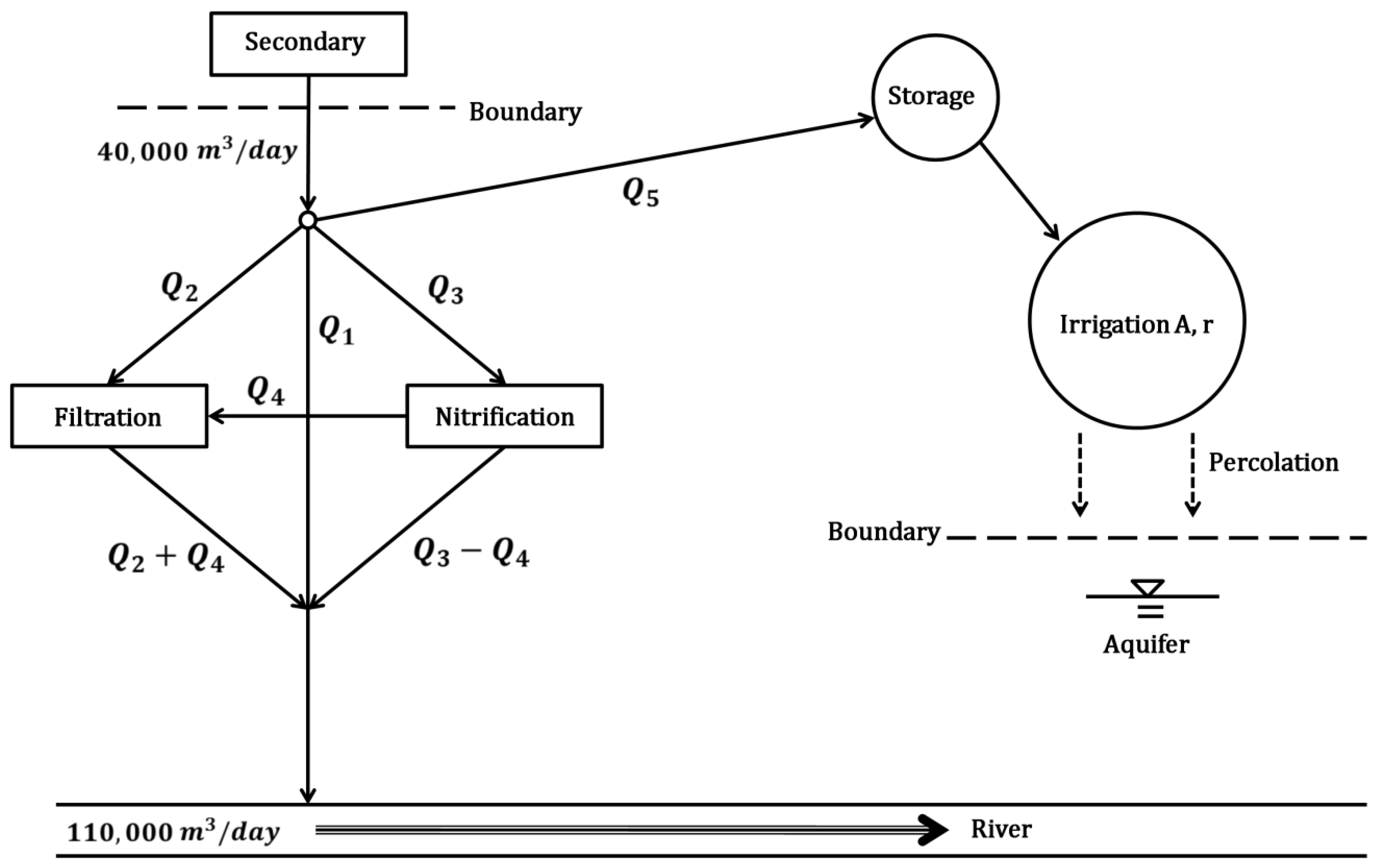
A city with the population of 100,000 people disposes of wastewater into a river. The wastewater of 40,000 m³/day is first treated with two operations of settling and biological oxidation to eliminate organic material. However, these treatments are not enough to satisfy the water quality standard of 5 ppm (or 5 mg/L) dissolved oxygen (DO) during summertime, which was set by regulation agencies for maintaining aquatic life. Thus, the city is forced to construct additional treatment systems to enhance the effluent quality.

The expanded wastewater treatment system consists of two additional treatment systems (filtration and nitrification) and one diverted irrigation system as shown in Figure 1. In the system, we have to decide five decision variables, including (1) wastewater amount discharged directly into the river ($Q_1$ 10³ m³/day); (2) wastewater amount treated by filtration operations ($Q_2$ 10³ m³/day); (3) wastewater amount treated by nitrification operations ($Q_3$ 10³ m³/day); (4) wastewater amount treated by both nitrification and filtration operations ($Q_4$ 10³ m³/day); and (5) wastewater amount diverted for irrigation and fertilization ($Q_5$ 10³ m³/day).

Table 1. Effluent quality after each treatment.

Treatment	Effluent Quality (ppm)
	DO	CBOD	NBOD
Secondary only ($Q_1$)	2	25	54
Secondary+Filtration ($Q_2$)	2	13	50
Secondary+Nitrification ($Q_3-Q_4$)	2	13	10
Secondary+Nitrification+Filtration ($Q_4$)	2	7	10

shows the effluent quality after each treatment.

Additionally, there exists one more decision variable $r$ which stands for irrigation rate (cm/week). For the diverted wastewater amount $Q_5$, the following mass balance equation can be considered:

$$Percolation=rT+P-ET$$

(1)

where $T$ is irrigation period (13 weeks in this study), $P$ is the precipitation amount (cm) during the irrigation period, and $ET$ is the evapotranspiration amount (cm) during the irrigation period ($ET$ is assumed to be equal to $P$ in this study). If the nitrogen concentration of the diverted amount $Q_5$ is $n$ (20 ppm in this study), the total nitrogen amount becomes $0.1rTn$ (kg/ha). If crop nitrogen uptake amount is $NC$ (170 kg/ha in this study), the surplus nitrogen amount of $Q_5$ becomes $0.1rTn-NC$, and the nitrate-nitrogen concentration $c_n$ (ppm) in the percolation amount becomes as follows:

$$c_n=\frac{surplusnitrogen}{percolation}=\frac{10(0.1rTn-NC)}{rT+P-ET}$$

(2)

Here, the city-regulated $c_n$ is less than or equal to 10 ppm for drinking water usage. Additionally, the nitrogen amount in $Q_5$ should be enough to cover the crop’s nitrogen requirement as follows:

$$0.1rTn\ge NC$$

(3)

For the discharged amount ($Q_1+Q_2+Q_3$) into the river, dissolved oxygen $C(x)$ at a distance ($x$ km) from the point of wastewater discharge can be expressed as the following differential equation:

$$u\frac{dC}{dx}=k_2(C_s-C)-k_{1}B-k_{n}N$$

(4)

where $u$ is river flow velocity (7.9 km/day in this study); $k_2$ is the re-aeration rate (0.5/day in this study); $C_s$ is saturation DO (8.0 ppm in this study); $B$ and $N$ are the remaining carbonaceous biochemical oxygen demand (CBOD) and nitrogenous biochemical oxygen demand (NBOD) (ppm) at distance $x$; and $k_1$ and $k_n$ are rate constants (0.35/day and 0.2/day, respectively). The first term on the right-hand side of Equation (4) denotes an oxygen increase due to re-aeration and the second and third terms denote an oxygen decrease due to oxidation of carbonaceous and nitrogenous material, respectively.

From the following relationship:

$$u\frac{dB}{dx}=-k_{1}B$$

(5)

$$u\frac{dN}{dx}=-k_{1}N$$

(6)

Equation (4) becomes:

$$\frac{dC}{dx}=\frac{k_2}{u}(C_s-C)-\frac{k_1}{u}{B}_0{e}^{-k_{1}x/u}-\frac{k_n}{u}{N}_0{e}^{-k_{n}x/u}$$

(7)

where $B_0$ and $N_0$ are, respectively, river CBOD and NBOD right after discharge. Additionally, Equation (7) can be rewritten in the format of a first-order non-homogeneous ordinary differential equation as follows:

$$\frac{dC}{dx}+\frac{k_2}{u}C=q(x),q(x)=\frac{k_2}{u}{C}_s-\frac{k_1}{u}{B}_0{e}^{-k_{1}x/u}-\frac{k_n}{u}{N}_0{e}^{-k_{n}x/u}$$

(8)

We can set an integral factor $\mu$ as follows:

$$\mu =e^{{\displaystyle \int \frac{k_2}{u}dx}}=e^{\frac{k_2}{u}x}$$

(9)

Then, if we multiply $\mu$ and both sides of Equation (8), it becomes as follows because $\frac{d\mu }{dx}=\frac{k_2}{u}\mu$:

$$\mu \frac{dC}{dx}+C\frac{d\mu }{dx}=\mu q(x)$$

(10)

Or, it becomes:

$$\frac{d}{dx}(\mu C)=\mu q(x)$$

(11)

If we integrate Equation (11), it becomes:

$$\mu C={\displaystyle \int \mu }q(x)dx+\tilde{C}$$

(12)

If we divide both sides of Equation (12) by $\mu$, it becomes:

$$C=\frac{1}{\mu }{\displaystyle \int \mu }q(x)dx+\frac{1}{\mu }\tilde{C}=e^{-\frac{k_2}{u}x}{\displaystyle \int e^{\frac{k_2}{u}x}}q(x)dx+\tilde{C}{e}^{-\frac{k_2}{u}x}$$

(13)

Here, ${\displaystyle \int e^{\frac{k_2}{u}x}}q(x)dx$ becomes:

$$\begin{array}{l}{\displaystyle \int \left(\frac{k_2}{u}{C}_s{e}^{\frac{k_2}{u}x}-\frac{k_1}{u}{B}_0{e}^{\frac{-k_1}{u}x}{e}^{\frac{k_2}{u}x}-\frac{k_n}{u}{N}_0{e}^{\frac{-k_n}{u}x}{e}^{\frac{k_2}{u}x}\right)}dx\\ =C_s{e}^{\frac{k_2}{u}x}-\frac{k_1}{k_2-k_1}{B}_0{e}^{\frac{k_2-k_1}{u}x}-\frac{k_n}{k_2-k_n}{N}_0{e}^{\frac{k_2-k_n}{u}x}+\tilde{\tilde{C}}\end{array}$$

(14)

Thus, Equation (13) becomes:

$$C=C_s-\frac{k_1}{k_2-k_1}{B}_0{e}^{\frac{-k_1}{u}x}-\frac{k_n}{k_2-k_n}{N}_0{e}^{\frac{-k_n}{u}x}+\tilde{\tilde{C}}{e}^{\frac{-k_2}{u}x}+\tilde{C}{e}^{\frac{-k_2}{u}x}$$

(15)

If $x=0$ and $D=\tilde{\tilde{C}}+\tilde{C}$, Equation (15) becomes:

$$C_0=C_s-\frac{k_1{B}_0}{k_2-k_1}-\frac{k_n{N}_0}{k_2-k_n}+D$$

(16)

where $C_0$ is the river DO right after discharge. Finally, we can obtain the analytic solution as follows. Actually, the name of the equation is Streeter–Phelps [21], which is also known as the DO sag equation, and first derived in 1925 based on data from the Ohio River. The model conveniently shows how DO decreases along the river reach by degradation of the biological oxygen demand (BOD).

$$\begin{array}{l}C(x)=C_s-\frac{k_1{B}_0}{k_2-k_1}{e}^{\frac{-k_1}{u}x}-\frac{k_n{N}_0}{k_2-k_n}{e}^{\frac{-k_n}{u}x}+\left(C_0-C_s+\frac{k_1{B}_0}{k_2-k_1}+\frac{k_n{N}_0}{k_2-k_n}\right)e^{\frac{-k_2}{u}x}\\ =C_s\left(1-e^{\frac{-k_2}{u}x}\right)+C_0{e}^{\frac{-k_2}{u}x}-\frac{k_1{B}_0}{k_2-k_1}\left(e^{\frac{-k_1}{u}x}-e^{\frac{-k_2}{u}x}\right)-\frac{k_n{N}_0}{k_2-k_n}\left(e^{\frac{-k_n}{u}x}-e^{\frac{-k_2}{u}x}\right)\end{array}$$

(17)

If river water and wastewater are completely mixed at the discharge point, the initial $C_0$, $B_0$, and $N_0$ can be calculated using a weighted average. Since the river flow is 110,000 m³/day, river DO is 8.0 ppm, river CBOD is 2.0 ppm, and river NBOD is 5.0 ppm, $C_0$, $B_0$, and $N_0$ become as follows:

$$C_0=\frac{8(110)+2(Q_1+Q_2+Q_3)}{110+Q_1+Q_2+Q_3}$$

(18)

$$B_0=\frac{2(110)+25Q_1+13Q_2+13(Q_3-Q_4)+7Q_4}{110+Q_1+Q_2+Q_3}$$

(19)

$$N_0=\frac{5(110)+54Q_1+50Q_2+10(Q_3-Q_4)+10Q_4}{110+Q_1+Q_2+Q_3}$$

(20)

The above-mentioned problem originally came from Haith [1]. However, because it does not reflect full aspects of the optimization procedure, this study modifies the problem by adjusting cost coefficients to obtain more reasonable optimization results.

3. Optimization Formulation

The objective function of this wastewater treatment problem is the total design cost of the system, which should be minimized while satisfying all the design constraints, as follows [1,8]:

$$\text{Minimize\hspace{1em}}z=f(Q_1,Q_2,Q_3,Q_4,Q_5,r)=C_{ft}+C_{nt}+C_{ir}$$

(21)

The objective function consists of three costs, such as filtration cost $C_{ft}$, nitrification cost $C_{nt}$, and irrigation cost $C_{ir}$. While many design optimization problems just consider initial capital (or construction) cost, this study considers life cycle costs, including operation and maintenance costs, crop sales benefit, and land rental fee.

The filtration cost $C_{ft}$ ($10³/year), which consists of capital costs (first term in right hand side) and operation and maintenance (O and M) costs (second term), is expressed as follow:

$$C_{ft}=1.5{(Q_2+Q_4)}^{0.93}+3.35{(Q_2+Q_4)}^{0.55}$$

(22)

The nitrification cost $C_{nt}$ ($10³/year), which consists of capital costs and O and M costs, is expressed as follow:

$$C_{nt}=6.9Q_3{}^{0.68}+5.3Q_3{}^{0.42}$$

(23)

The irrigation cost $C_{ir}$ ($10³/year), which consists of capital cost of transmission pipe, capital cost of the storage system, O and M costs of the storage system, capital cost of irrigation system, O and M costs of the irrigation system, and net benefit of crop farming (crop sales minus land rent), is expressed as follow:

$$\begin{array}{l}{C}_{ir}=21.9Q_5^{0.28}+1.2Q_5^{0.78}+0.2Q_5^{0.54}\\ +(13.1+48/r)Q_5^{(0.74+0.32/r)}+(5.1+19/r)Q_5^{(0.79+0.28/r)}-0.68A\end{array}$$

(24)

where $A$ is the irrigated area (ha), which can be calculated as $70Q_5/r$. Constraints for this problem are:

$$Q_1+Q_2+Q_3+Q_5=40$$

(25)

$$Q_3\ge Q_4$$

(26)

$$0\le Q_i\le 40,i=1,\dots ,5$$

(27)

$$\begin{array}{l}8(1-e^{-0.063x})+C_0{e}^{-0.063x}-2.33B_0(e^{-0.044x}-e^{-0.063x})\\ -0.67N_0(e^{-0.025x}-e^{-0.063x})\ge 5\end{array}$$

(28)

$$6.54\le r\le 13.07$$

(29)

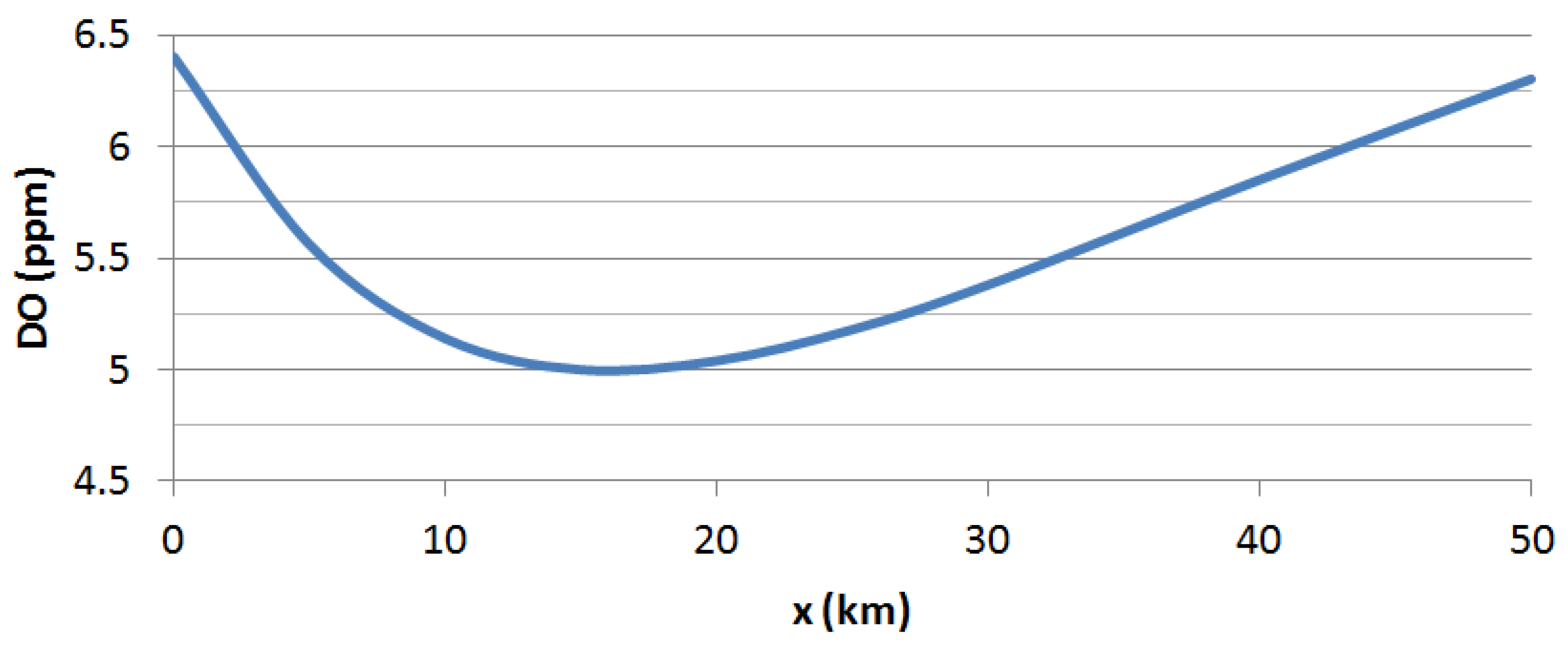
The constraint in Equation (25) represents that total wastewater amount is equal to 40,000 m³/day; the constraint in Equation (26) represents that the amount for nitrification should be greater than, or equal to, that for both nitrification and filtration; the constraint in Equation (27) represents that any individual amount cannot exceed the total amount as a non-negative value; the constraint in Equation (28) represents that DO concentration at any point ($x$ km downstream from the discharged point) should be greater than or equal to 5 ppm as regulated. In reality, we cannot test all the points because the number of them is astronomical. Thus, we instead test eight points with an even interval (5 km or 10 km) as previous studies did, which contain the DO sag curve; and the constraint in Equation (29) represents that the nitrate-nitrogen concentration $c_n$ should be less than, or equal to, 10 ppm as in Equation (2) and the total nitrogen amount should be greater than, or equal to, the crop nitrogen requirement as in Equation (3).

4. Parameter-Setting-Free Harmony Search

The basic harmony search algorithm starts with a solution pool named harmony memory (HM), where randomly generated and feasible solutions are initially filled to the size of the harmony memory (HMS; 30 in this study) as follows [8]:

$$HM=\left[\begin{array}{cccccc}{Q}_1^1& Q_2^1& Q_3^1& Q_4^1& Q_5^1& r^1\\ Q_1^2& Q_2^2& Q_3^2& Q_4^2& Q_5^2& r^2\\ ⋮& ⋮& ⋮& ⋮& ⋮& ⋮\\ Q_1^{HMS}& Q_2^{HMS}& Q_3^{HMS}& Q_4^{HMS}& Q_5^{HMS}& r^{HMS}\end{array}|\begin{array}{c}f(x^1)\\ f(x^2)\\ ⋮\\ f(x^{HMS})\end{array}\right]$$

(30)

Next, a new harmony (solution vector) $x^{New}$ is improvised based on HM as follows:

$$x_i^{New}\leftarrow \{\begin{array}{ccc}{x}_i\in [x_i^{Lower},x_i^{Upper}]& \mathrm{w}.\mathrm{p}.& (1-HMCR)\\ x_i\in HM=\{x_i^1,x_i^2,\mathrm{...},x_i^{HMS}\}& \mathrm{w}.\mathrm{p}.& HMCR\cdot (1-PAR)\\ x_i+\Delta ,x_i\in HM& \mathrm{w}.\mathrm{p}.& HMCR\cdot PAR\end{array},i=1,\dots ,6$$

(31)

where $\Delta$ is the pitch adjusting amount, which is calculated as $(x_i^{Upper}-x_i^{Lower})/1000\times u(-1,1)$ in this study ($u(-1,1)$ is uniform random number between −1 and 1), HMCR denotes a harmony memory considering rate (0 ≤ HMCR ≤ 1) and PAR denotes pitch adjusting rate (0 ≤ PAR ≤ 1). In memory considering operation, any value in HM can be selected using uniform random index $int(HMS\times u(0,1))+1$ ($int(\cdot )$ is integer function which returns the integer portion of a number).

If the newly generated harmony $x^{New}$ satisfies all the constraints and is better than the worst harmony $x^{Worst}$ stored in HM, the former replaces the latter as follows:

$$x^{New}\in HM\wedge x^{Worst}\notin HM$$

(32)

The basic HS algorithm repeats Equations (31) and (32) until a termination criterion is satisfied.

In this study, the PSF-HS algorithm has one more matrix, named operation type matrix (OTM), as follows:

$$OTM=\left[\begin{array}{cccc}{o}_1^1=Random& o_2^1=Pitch& \cdots & o_6^1=Memory\\ o_1^2=Memory& o_2^2=Memory& \cdots & o_6^2=Pitch\\ ⋮& \cdots & \cdots & \cdots \\ o_1^{HMS}=Memory& o_2^{HMS}=Random& \cdots & o_6^{HMS}=Memory\end{array}\right]$$

(33)

OTM retains the operation (memory consideration, pitch adjustment, or random selection) by which each variable value is obtained. At the early stage of computation (for example, number of iterations is less than 4 × HMS), HMCR and PAR are fixed into 0.5 and OTM are being updated. Then, after the early stage, based on OTM, HMCR, and PAR are iteratively calculated, instead of using fixed values, as follows:

$$HMC{R}_i=\frac{ct\left(o_i^j=Memory\vee o_i^j=Pitch,\forall j\right)}{HMS}$$

(34)

$$PA{R}_i=\frac{ct\left(o_i^j=Pitch,\forall j\right)}{ct\left(o_i^j=Memory\vee o_i^j=Pitch,\forall j\right)}$$

(35)

where $ct(\cdot )$ denotes the function which counts the number of designated operation.

Since each decision variable has its own HMCR and PAR, Equation (31) should be slightly modified as follows:

$$x_i^{New}\leftarrow \{\begin{array}{ccc}{x}_i\in [x_i^{Lower},x_i^{Upper}]& \mathrm{w}.\mathrm{p}.& (1-HMC{R}_i)\\ x_i\in HM=\{x_i^1,x_i^2,\mathrm{...},x_i^{HMS}\}& \mathrm{w}.\mathrm{p}.& HMC{R}_i\cdot (1-PA{R}_i)\\ x_i+\Delta ,x_i\in HM& \mathrm{w}.\mathrm{p}.& HMC{R}_i\cdot PA{R}_i\end{array},i=1,\dots ,6$$

(36)

5. Computation Results

In previous research [8], the basic HS algorithm, which was applied to the optimal design of the wastewater treatment system for river conservation, found good solutions while GRG got stuck in local optima, or even diverged.

However, the solution quality of the basic HS algorithm was influenced by the algorithm parameter values to some degree. With good parameters (HMCR = 0.95, PAR = 0.3, iterations = 10,000, and 10 runs), the basic HS algorithm found the best solution of 302.1 ($10³/year) and the average solution of 302.4 ($10³/year). Meanwhile, with worse parameters (HMCR = 0.5, PAR = 0.5, iterations = 10,000, and 10 runs), it found the best solution of 308.2 ($10³/year) and the average solution of 312.7 ($10³/year).

To make matters worse, the original approach had a tendency to choose only $Q_1$ (no treatment) and $Q_5$ (irrigation) without choosing $Q_2$ (filtration) or $Q_3$ (nitrification). In other words, although we elaborate the filtration and nitrification treatment formulation, it is useless if it is not chosen in optimization process. Thus, a couple of cost functions (Equations (22) and (23)) were modified in order for every decision variable to have certain value.

When the PSF-HS approach (iterations = 5000 and 10 runs) in this study was applied to the modified real-scale wastewater treatment problem, it was able to find good solutions with the best solution of 175.18 ($10³/year) and the average solution of 207.87 ($10³/year). PSF-HS successfully produced the solutions without demanding the tedious algorithm parameter setting process.

Table 2. Optimization results by PSF-HS.

Run No.		#1	#2	#3	#4	#5	#6	#7	#8	#9	#10
Total Cost (k$/year)		235.54	210.31	190.13	217.26	248.77	200.63	175.18	207.85	176.51	216.55
$Q_1$ (k ton/day)		0.16	0.28	0.19	0.45	0.34	0.34	0.19	0.87	0.12	0.30
$Q_2$ (k ton/day)		0.44	0.54	1.30	0.37	0.88	0.34	0.68	0.43	0.54	0.49
$Q_3$ (k ton/day)		35.66	38.17	38.44	37.70	33.56	38.80	39.14	38.08	39.34	37.75
$Q_4$ (k ton/day)		22.49	31.78	37.49	30.77	21.38	32.67	34.64	36.41	33.53	30.27
$Q_5$ (k ton/day)		3.74	1.00	0.07	1.48	5.22	0.52	0.00	0.63	0.00	1.47
$r$ (cm/week)		13.07	13.07	11.75	12.96	13.07	13.07	6.54	13.07	13.07	13.07
Crop Nitrogen (≥ 170 kg/ha)		339.82	339.82	305.47	336.83	339.82	339.82	170.04	339.82	339.82	339.82
Percolation $c_n$ (≤ 10 ppm)		9.99	9.99	8.87	9.91	9.99	9.99	0.00	9.99	9.99	9.99
$x$ km (≥ 5 ppm)	5	5.61	5.57	5.56	5.58	5.64	5.56	5.56	5.57	5.56	5.58
	10	5.16	5.14	5.14	5.15	5.17	5.14	5.14	5.14	5.14	5.15
	15	5.00	5.00	5.00	5.00	5.00	5.00	5.00	5.00	5.00	5.00
	20	5.03	5.03	5.04	5.03	5.02	5.04	5.04	5.03	5.04	5.03
	25	5.16	5.17	5.18	5.17	5.15	5.18	5.18	5.17	5.18	5.17
	30	5.36	5.38	5.38	5.37	5.35	5.38	5.38	5.37	5.38	5.37
	40	5.83	5.84	5.84	5.84	5.82	5.85	5.85	5.84	5.85	5.84
	50	6.29	6.29	6.29	6.29	6.27	6.30	6.30	6.29	6.30	6.29

shows the computational results of 10 runs from PSF-HS.

The best solution ($175.18 × 10³/year) of PSF-HS with the solution vector ($Q_1$ = 0.2; $Q_2$ = 0.7; $Q_3$ = 39.1; $Q_4$ = 34.6; $Q_5$ = 0.0; $r$ = 6.5) satisfies the minimum DO requirement constraint (DO ≥ 5 ppm) specified in Equation (28) at all river reaches, the maximal nitrate-nitrogen concentration constraint (0.0 ppm ≤ 10 ppm) specified in Equation (2), and the minimal nitrogen requirement constraint specified in Equation (3) (170.04 kg/ha ≥ 170 kg/ha). Figure 2 shows DO sag curve of the best solution ($175.18 × 10³/year), which satisfies the minimal DO constraint.

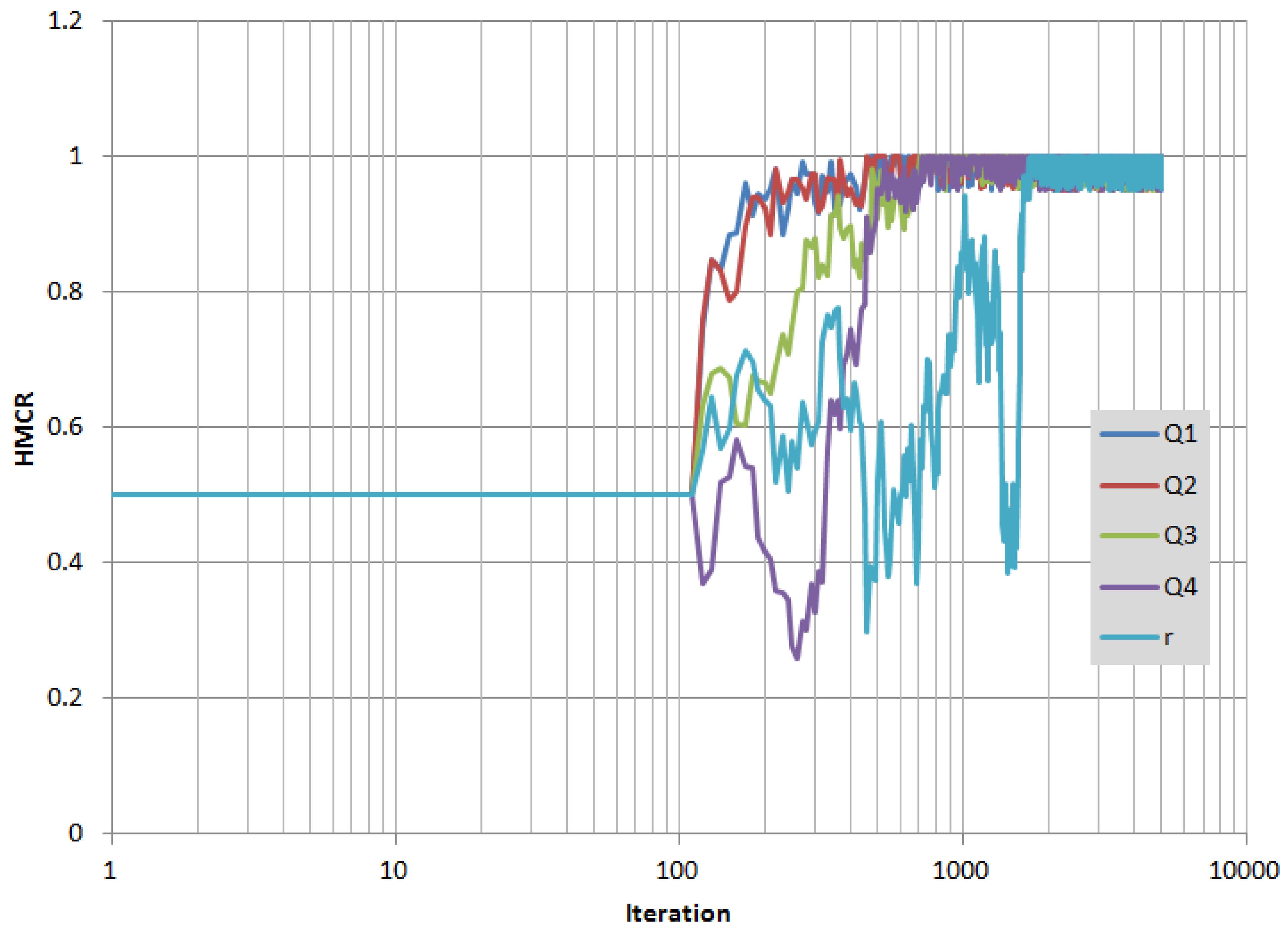
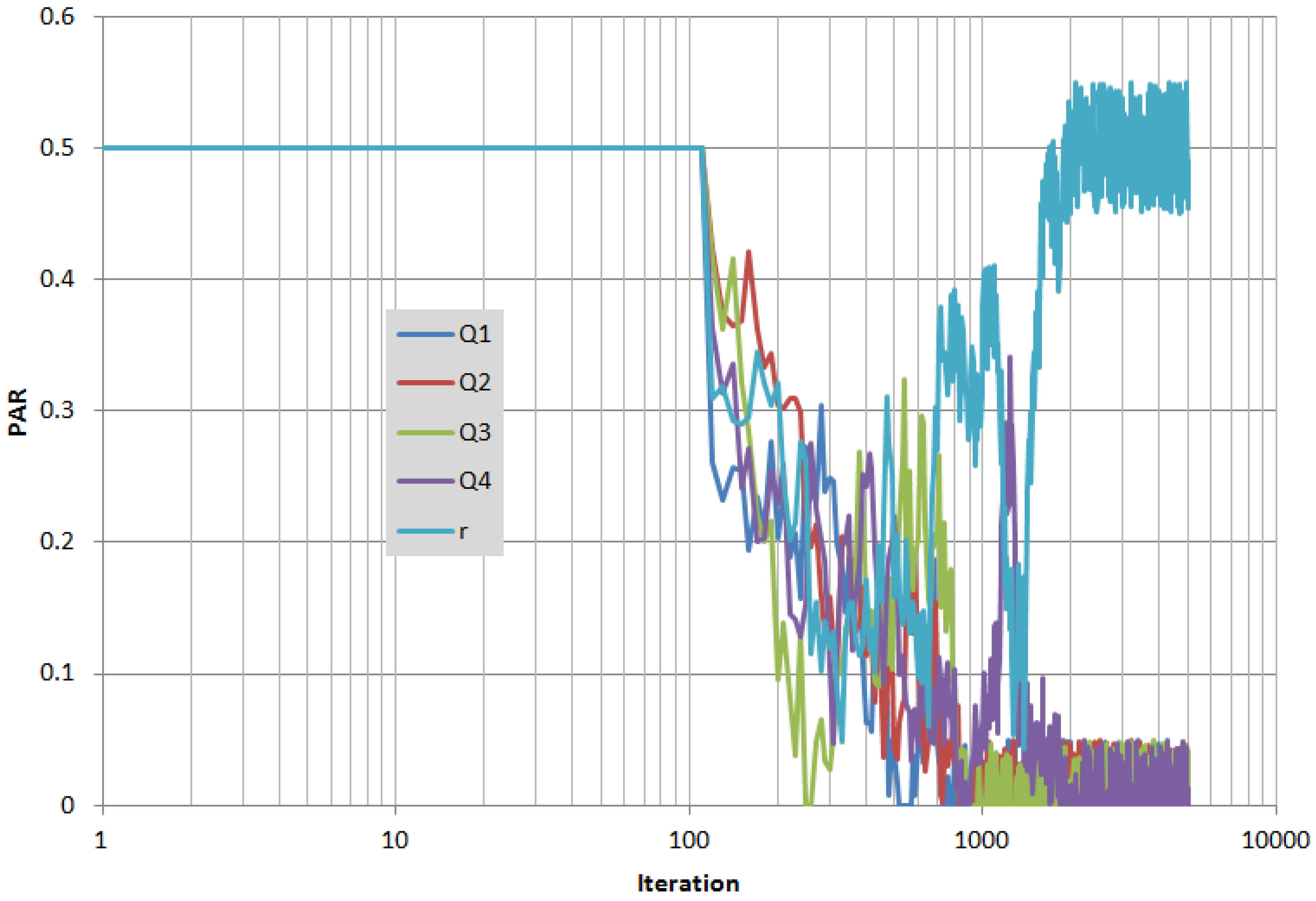
Figure 3 and Figure 4 show the trends of HMCR and PAR, which have been automatically adapted, as the iteration goes.

As seen in Figure 3, all HMCR’s have converged into higher values (more than 0.95) after 2000 iterations. Meanwhile, as seen in Figure 4, all PARs, except that from irrigation rate $r$, came down to lower values between 0.0 and 0.05 after 2000 iterations. The PAR for irrigation rate $r$ soared to around 0.5 after fluctuating between 0.05 and 0.4.

6. Conclusions

For river sustainability, a wastewater treatment system, which has three different options of treatments, such as filtration, nitrification, and diverted irrigation, was optimally designed using the PSF-HS technique which does not require the tedious task of algorithm parameter value setting.

When the PSF-HS technique was applied to the system, it could find the lowest cost design while satisfying the minimal DO requirement in the river, maximal nitrate-nitrogen concentration in groundwater, and the minimal nitrogen requirement for crop farming by automatically adapting its parameter values. This user-friendliness can help any designer/engineer to more easily use this model in real-world design process.

For future study, more realistic and up-to-date wastewater treatment systems can be considered and more robust PSF-HS techniques are expected to be developed. Additionally, because the optimization model in this study searches for the minimal budget solution in terms of life cycle costs (construction, operation, and management costs), while satisfying environmental criteria, the general format of this model can possibly be applied to other sustainability problems, such as a waste-disposal plant design.