Multi-Regional Input-Output (MRIO) Study of the Provincial Ecological Footprints and Domestic Embodied Footprints Traded among China’s 30 Provinces

Abstract

Rapid development in China has led to imbalances and inequities of ecological resources among the provinces and regions. In this study, an environmentally extended multi-regional input-output (MRIO) model was used to analyze the imbalances, inequities and pressures of the ecological footprints (EF) of China’s 30 provinces in 2007. In addition, by decomposing the total product consumption coefficients, we calculated the net embodied EF of the flows among the provinces by the total amount, land type and sector. The results showed that most provinces presented EF deficits. Significant differences were observed between the ecological pressure in consumption (EPC) and ecological pressure in production (EPP) for each province because of the net embodied EF trade; the EPCs of Shanghai (15.16), Beijing (7.81) and Tianjin (7.81) were the largest and presented descending EPPs, whereas the EPCs of Heilongjiang (0.98), Hebei (0.98), Xinjiang (0.98) and Guangxi (0.98) were under the threshold value (1) and presented ascending EPPs. The carbon footprint in the secondary sector was the main embodied EF of the flows among the provinces responsible for inequities. Finally, based on the various conditions of the provinces in different geographical regions, we have provided suggestions for regionally balanced development that can maintain the EPP and EPC values under the threshold for each province.

1. Introduction

The sustainable development of global resources and the environment, balanced usage of resources and environmental fairness among countries and regions are becoming increasingly important issues. Regarding the sustainable development of the ecological environment, polluter-pays and consumer-pays principles have been discussed in many studies [1]. In recent years, first, the division of ecological responsibility based on consumption has been well recognized and appears to be more reasonably managed. In addition, second, consumers have become more aware of the embodied content of ecological resources in their daily consumption habits, and the overall awareness of ecological protection issues has been improved. Moreover, ecological responsibility in production practices cannot be ignored because local ecological destruction is directly caused by these practices’ content. To quantify the depletion of ecological resources, ecological footprints (EFs) are analyzed in this study.

The concept of an EF was initially proposed by Rees [2] and Wackernagel [3] in the 1990s as a land resource accounting tool that is based on consumption and is capable of tracking the impact of local consumption on ecology and the environment and promoting policies for sustainability. Currently, the EF model has been calculated at different scale levels, including the national, sub-national, city and campus level, and the method has been improved in many studies, such as by the concepts of exergy [4,5,6], emergy [7], net primary productivity [8,9,10,11] and input-output analysis (IOA). In thermodynamics, the exergy of a system is the maximum useful work possible during a process that brings the system into thermodynamic equilibrium with the surrounding environment [12]. The modified EF by exergy is calculated by summarizing all the exergy content in all kinds of substance and energy in the consumption of social terminal/end products and services. Then, the conversion factor of exergy to EF is used to calculate the corresponding EF [4]. According to the Odum Emergy theory [13], all terminal products’ and services’ consumption can be transferred into uniform solar emjoules (sej), which could be further converted to an EF by using the conversion factor of emergy to EF. As far as net-primary-productivity-based EFs are concerned, they focus on the improvement of the yield factor and equivalence factor, whereas IOA-based methods serve as better options to study the flow difference in the industry. Nevertheless, the mainstream EF method is the National Footprint Accounting (NFA) method developed by the Global Footprint Network (GFN), which mainly focuses on issues at the national scale. For China, an increasing number of studies of sub-national EFs have emerged; however, issues related to assessing sub-national EFs via the NFA remain [14].

Weinzettel et al. [15] compared the differences in the national EF calculated by the NFA, multi-regional input-output (MRIO) and hybrid-MRIO methods and indicated that the main drawbacks of the NFA are the EFs of imported and exported products, including the yield factor (YF) of traded products, a reduced number of products used in the calculation and the embodied EFs in the trade products. Wiedmann [16] indicated that EF calculations should include three levels: first, the direct use of the local EF; second, the embodied EF in product trade; and third, all embodied EFs of all the products, including local products with embodied external EFs. Although the NFA’s method does not consider the third level, in the calculation of China’s sub-national (regional) EFs because of the non-comprehensive local production data and lack of interprovincial trade data, accurately calculating local EFs are still difficult, which decreases the relevance of many associated studies and results in a loss of information related to embodied EFs in the intermediate link between local and external regions.

The environmentally extended multi-regional input-output (EE-MRIO) model was first introduced by Lenzen et al. [17]. The EE-MRIO model has been applied to environmental issues in many studies. To calculate the CO₂ emissions, Xi and Xie calculated the carbon footprints of eight regions in China in 2007 [18,19]. Zhang and Anadon used the EE-MRIO model to analyze Chinese domestic water footprint trade [20]. Giljum, Bruckner and Aldo Martinez [21] utilized the EE-MRIO to calculate global material consumption. Wilting used the model to calculate the consumption of land use and carbon emissions in The Netherlands [22]. Studies related to EFs [15] were also performed. Weinzettel and Steen-Olsen [23] created an assessment model to track global anthropogenic pressure by analyzing EFs, carbon footprints and water footprints with the EE-MRIO model. Galli et al. [24] proposed a framework for a footprint family based on the EE-MRIO to evaluate global sustainable development. A comparison of carbon and water footprint calculations indicated that integrating EFs into the EE-MRIO footprint family framework is imperative. Ewing [25] combined EFs and water footprints with a MRIO model. Although most of above studies were performed at the national level, they can be applied to research at the sub-national level [26].

With the rapid development of China’s economy, issues related to monitoring and protecting the environment have received increasing attention. Many studies on China’s EF have focused on comparisons with other countries at national and regional scales; however, studies of the interregional EF within China are rare. Because of the differences and imbalances between China’s regional or provincial industrial structures, economic levels and ecological endowments, the differences of regional EFs, biocapacities, EF intensities and embodied EF transferal paths must be evaluated.

In this paper, the EE-MRIO model was adopted to study China’s EF and its flow so as to assess the imbalances and inequities of EFs and related ecological issues. According to EE-MRIO theory, in the method, (1) external and local footprints can be distinguished comprehensively; (2) the missing footprints calculated by the NFA, mainly the embodied EFs of the intermediate link, can be tracked; (3) issues of interregional trade data can be overcome; and (4) it is convenient and effective to obtain each flow of EF among regions and sectors. EE-MRIO is just suitable for the issues to be solved in this paper. By taking advantage of the merits of EE-MRIO, the local and external provincial direct and embodied EFs can be comprehensively calculated. The following specific work has been done in this paper:

(1)

The provincial EF and biocapacity (BC) calculated by the EE-MRIO can be used to demonstrate differences in the EF and per capita EF among the provinces. The EF and corresponding BC data are used to quantitatively investigate the ecological pressure (EP) in consumption and production.

(2)

The net embodied interprovincial EF calculated by total amount, sector and EF type according to the EE-MRIO model are used to track details of China’s embodied EF trade in 2007.

(3)

The EP based on consumption and production contexts is analyzed to offer a quantitative basis by which ecological environment protection promotes sustainable consumption [27] and production.

2. Materials

2.1. Study Areas and Sectors

Because of the lack of energy data in Tibet as well as the lack of an input-output table in this paper, the research scope consists of China’s 30 provinces (excluding Hong Kong, Macao, Taiwan, Tibet, and part of Sansha Islands).

Based on the socioeconomic development of the different regions, China State Council provided the basis for regional development policies by “promoting the rise of the central region based on a number of opinions” [28], “issuing a number of policies and measures on the western development implementation of policies” [29] and the promoting the spirit of the Party Congress report. Currently, China’s economic regions are divided into the northeast, eastern, central and western regions [30]. As shown in Figure 1, the areas are divided as follows: the northeast region includes Liaoning, Jilin and Heilongjiang; the eastern region includes Beijing, Tianjin, Hebei, Shanghai, Jiangsu, Zhejiang, Fujian, Shandong, Guangdong and Hainan; the central region includes Shanxi, Anhui, Jiangxi, Henan, Hubei and Hunan; and the western region includes Inner Mongolia, Guangxi, Chongqing, Sichuan, Guizhou, Yunnan, Tibet, Shaanxi, Gansu, Qinghai, Ningxia and Xinjiang.

The six sectors are agriculture, industry, construction, transportation and warehousing, wholesale and retail, and other services as shown in

Table 1. China’s six sectors in 2007.

Sector	Abbreviation	Sector	Abbreviation
Farming, Forestry, Animal Husbandry, and Fishing	Agriculture	Transportation and Warehousing	Transportation
Industry	Industry	Wholesale and Retail	Sales
Construction	Construction	Other Services	Other

.

2.2. Data and Processing

2.2.1. Data Sources

Compiling MRIO data represents a complex project, and the most recent project is the China multi-region input-output table for 2007, which was sourced from Liu et al.’s research China’s 30 provinces and autonomous regions in 2007: Regional Input-Output Table Compilation Theory and Practice [31]. This table contains 30 Chinese provinces and six sectors. The data required for the environmentally extended matrix are all derived from direct production, including the production of arable land, forests, grazing land, fishing areas, built-up land, and tons of CO₂ emissions. Therefore, the following statistical data should be collected. (1) Data for the provincial production (kg) and yield (kg/ha) of arable, forest, grazing, fishing, and built-up land by product are sourced from the China Agriculture Yearbook 2008 [32] and the China Statistical Yearbook 2008 [33]. The direct and intermediate provincial energy consumption data are sourced from the provincial energy balance in the China Energy Statistical Yearbook 2008 [34]; (2) Data for the provincial and available arable, forest, grazing, fishing, and built-up land in 2007 are sourced from the China Statistical Yearbook 2008 [33]; and (3) data for the provincial Gross Domestic Product (GDP) and population and sectoral data for the provincial GDP are sourced from the China Population and Employment Statistics Yearbook 2008 [35] and the China Statistical Yearbook 2008 [33].

2.2.2. Land Data Processing

Table 2. Items and sub-items for each land type.

Land Type	Items	Sub-Items
Arable	Food crops	Rice, wheat, corn, millet, sorghum, other grains, soybeans, potatoes
	Oil crops	Rapeseed, peanuts, sesame, sunflowers, Hu Mazi
	Hemp	Yellow kenaf, ramie, flax, hemp
	Sugar	cane, beet
	Other	Tobacco, cotton
Forest	Fruit	Apples, oranges, pears, grapes, bananas
	Wood	Wood, bamboo, timber, artificial board
Grazing	Animal products	Beef, mutton, poultry, milk, eggs, honey
Fishing	Seafood	Fish, shellfish, algae
Carbon	Carbon uptake	Raw coal, cleaned coal, coal briquettes, coke, coke oven gas, crude oil, gasoline, kerosene, diesel oil, fuel Oil, PLG, refinery gas, natural gas
Build-up	Build-up	Residential land, industrial and mining land, transportation land, land for water conservancy facilities

shows the items and sub-items for each land type. According to the national average yield, the provincial domain data are converted into the number of hectares for the national average yield. According to Liu et al. [36], the YF and the equivalence factor (EQF) are adopted in the WWF’s Living Planet Report 2006 [37].

Table 3. Yield factor (YF) and equivalence factor (EQF) for each land type.

	Arable/Built-Up Land	Forest/Carbon Land	Grazing Land	Fishing Land
YF	1.74	0.86	0.51	0.74
EQF	2.21	1.34	0.49	0.36

The YF represents the conversion factor of the local yield per unit area for a certain product to its world average yield. And EQF is the factor with which the ecological footprint (EF) of land use types with different productivity could be converted into unified unit with global average productivity.

lists the data for the YF and EQF used in this study.

2.2.3. Energy Data Processing

According to the energy balance sheet classifications [34], 17 types of energy are investigated in this study: raw coal, cleaned coal, washed coal, coal briquettes, coke, coal coke, other gas, crude oil, gasoline, kerosene, diesel oil, fuel oil, liquefied petroleum gas (LPG), refined oil, natural gas, petroleum and coking coal. The oxidation rates are from A Guide of the Compilation of Provincial Greenhouse Gas Inventory for Low Carbon Development [38], which was edited by the National Development and Reform Commission. We employ the average low calorific value data from the China Energy Statistical Yearbook 2008. The emission factors are adopted from the IPCC’s 2006 recommendations [39].

To avoid calculating the primary energy and corresponding secondary energy twice, the sector for energy transformation should be calculated as shown below. According to the classification of the energy balance table in the China energy statistical yearbook, the energy sectors of transformation are as follows: thermal power, heating supply, coal washing, coking, petroleum refineries, gas works and coal product processing. The main task is to calculate the transformation emission coefficients of coking and petroleum refineries, which are represented by 0.406 tCO₂/t (tons of carbon dioxide per one ton of energy) for coke [40] and 0.312 tCO₂/t for petroleum [41] in this study. The fuel conversion of thermal power generation and heating can be directly calculated, and the direct emissions of washed coal, gas, and coal product processing can be ignored because they produce low levels of carbon emissions.

3. Methods

3.1. Indicators

(1) EFs of Production

There are six types of EFs related to production: arable land, forest, fishing, grazing land, carbon land and built-up land [42]. The EFs of production for the first four land types can be calculated with Formula (1), and the EF for carbon land can be calculated with Formula (2).

$$E{F}_P={\displaystyle \sum _i\frac{P_i}{Y_i}}\cdot Y{F}_i\cdot EQ{F}_i$$

(1)

where $P_i$, $Y_i$, $Y{F}_i$ and $EQ{F}_i$ represent the annual production, national average yield, yield factor and equivalence factor for land type of product $i$, respectively.

$$E{F}_{P,carbon}=\frac{P_c\cdot (1-S_{ocean})}{Y_c}EQ{F}_{carbon}$$

(2)

where $P_c$ denotes the regional carbon emissions per year, $Y_c$ is the global forest average carbon uptake capacity, and $S_{ocean}$ refers to the proportion of global human carbon emissions absorbed by the ocean. According to the calculation of GFN 2007, the oceans absorbed 28% of the global CO₂ emissions [42].

(2) Biocapacity

BC denotes the capacity of a region to support the human consumption of ecosystem services within ecologically productive land areas and the ability of a region to regenerate ecological resources and land services for human use, and it is the main unit used to assess sustainability in EF methods [43]. BC is calculated as follows:

$$BC={\displaystyle \sum _i{A}_i\cdot Y{F}_i\cdot EQ{F}_i}\cdot (1-BD)$$

(3)

where $A_i$ is the available area (in actual hectares) for the production of product $i$ in a region; $Y{F}_i$ is region-specific yield factor; $EQ{F}_i$ is the equivalence factor for converting the average productivity area of each EF type into global hectares of the average productivity for all EF types, and BD is a constant for the conservation occupancy of biological diversity (13.4% in this study) [44].

(3) Ecological Pressure

BC is a threshold indicator that is compared with the corresponding EF and used to assess whether a region is in an ecologically sustainable state; if not, it is also used to compare the differences among regions to quantify the degree of sustainability. EP is the ratio of local EF to local BC and indicates the number of years required by the environment to convert the EF of local human interactions to achieve a sustainable state. Niccolucci’s [45,46] use of a 3D EF model is similar in expression to EP and an intuitive method of expressing the relationship between EF, ecological deficits (ED; and ED = EF − BC, when EF > BC) and BC. For simplicity, we use EP to analyze the degree of sustainability for each of the studied regions.

$$EP=\frac{EF}{BC}$$

(4)

when the EP of a region is equal to or less than 1, it is in a state of sustainable development; otherwise, it is beyond the local BC. In this study, we consider the EP both from two different perspectives: from the ecological pressure in consumption (EPC) perspective, and that of an ecological pressure in production (EPP) perspective.

(4) Ecological Footprint Intensity (EFI)

EFI is the ratio of the total amount of the local EF to the local gross domestic product (ten thousand yuan) as calculated in Formula (5), and it indicates the ecological depletion in gha for one unit of GDP production. Larger values are correlated with lower eco-efficiency.

$$EFI=\frac{EF}{GDP}$$

(5)

3.2. Methods of Ecological Footprint (EF) Calculation with the Environmentally Extended Multi-Regional Input-Output (EE-MRIO) Model

Figure 2 shows the framework for calculating EFs based on the EE-MRIO. And the process can be divided into three steps:

The first step is about the construction of an environmentally-extended matrix. The direct energy consumption or agricultural (arable, forest, grazing and fishing) harvest (which could result in direct land appropriation or direct carbon emission and it is calculated as product quantity in the physical unit before being converted into land area) of each product in Table 2 is assigned to the row vector of the matrix first by region and then by sector. For all regions, the direct energy consumption of each sector is assigned with the energy data as cited in Section 2.2.3. Built-up land is divided into industrial, commercial, transportation. And water conservancy facilities are assigned into the sectors of industry, transportation, sale and agriculture, respectively. We adopted the first approach in product allocation as discussed by Weinzettel [23], since it is easy and independent of regional trade data to allocate the products to producing sectors. Based on the approach, the direct production of all products generated by arable land, forest land, grazing land and fishing land is assigned to the agriculture sector because all these products come from direct land appropriation. The second step is the calculation of direct product consumption coefficient and total product consumption coefficient for each product from each sector in each region which were discussed at length in Section 3.2.2. The final step is to covert the embodied product consumption, which was obtained by EE-MRIO, into corresponding EF according to Formulas (12)–(15) explained in Section 3.2.3.

In this study, due to varied YF in each region, the product consumption is not transferred into corresponding land use area except for built-up land in MRIO calculation. Also, built-up land is calculated by actual area directly. In order to facilitate the presentation, “consumption of a product related to EF” or “consumption of a product (EF)” (calculated as in the physical unit) is used to express the consumption of EF in production of agricultural harvest, consumption of energy and land appropriation of built-up. In other words, the land appropriation of the six land use types are expressed in the form of product consumption firstly before being transferred into EF.

3.2.1. Construction of EE-MRIO

Below lists the common used superscripts and subscripts in Section 3.2.

• $m$: the number of total regions
• $n$: the number of total sectors
• $r$, $s$: region identifier
• $i$, $j$: sector identifier
• $k$: product identifier.

Table 4. Structure of China’s interregional input-output table with the environmentally extended matrix in 2007.

		Intermediate Demand	Final Use	Total Output
		s: 1, 2, …, m	s: 1, 2, …, m
Intermediate input	r:	$Z^{rs}$	$F^{rs}$	$X^r$
	1
	2
	…
	m
Total input		$X^s$
Environmentally extended matrix (Products in physical units):		$P^s$	$P^{fs}$

shows the structure of China’s interregional input-output table with an environmentally extended matrix in 2007. The direct consumption coefficient ${\mathrm{a}}_{ij}^{rs}$ expresses the direct consumption from producing one monetary unit of production of sector $j$ in region $s$ from sector $i$ in region $r$ as follows:

$${\mathrm{a}}_{ij}^{rs}=\frac{z_{ij}^{rs}}{x_j^s}(r,s=1,2,...,m;i,j=1,2,...,n)$$

(6)

where $z_{ij}^{rs}$ is the intermediate consumption from sector $i$ in region $r$ to sector $j$ in region $s$ and $x_j^s$ is the total consumption of sector $j$ in region $s$.

$$\begin{array}{l}Let:A^{rs}=\left[\begin{array}{cccc}{a}_{11}^{rs}& a_{12}^{rs}& \dots & a_{1n}^{rs}\\ a_{21}^{rs}& a_{22}^{rs}& \dots & a_{12}^{rs}\\ ⋮& ⋮& \ddots & ⋮\\ a_{n1}^{rs}& a_{n2}^{rs}& \dots & a_{nn}^{rs}\end{array}\right],A=\left[\begin{array}{cccc}{A}^{11}& A^{12}& \dots & A^{1m}\\ A^{21}& A^{22}& \cdots & A^{2m}\\ ⋮& ⋮& \ddots & ⋮\\ A^{m1}& A^{m2}& \dots & A^{mm}\end{array}\right]\\ \\ F^{rs}=\left(\begin{array}{c}{f}_1^{rs}\\ f_2^{rs}\\ ⋮\\ f_n^{rs}\end{array}\right), F=\left[\begin{array}{cccc}{F}^{11}& F^{12}& \cdots & F^{1m}\\ F^{21}& F^{22}& \cdots & F^{2m}\\ ⋮& ⋮& \ddots & ⋮\\ F^{m1}& F^{m2}& \cdots & F^{mm}\end{array}\right]\\ \\ X^r=\left(\begin{array}{c}{x}_1^r\\ x_2^r\\ ⋮\\ x_m^r\end{array}\right), X=\left[\begin{array}{c}{X}^1\\ X^2\\ ⋮\\ X^m\end{array}\right]\end{array}$$

where $A^{rs}$ and $F^{rs}$ express the sub-matrices of intermediate consumption and final consumption, respectively, from region $r$ to region $s$; and $f_i^{rs}$ indicates the final consumption of region $s$ from sector $i$ in region $r$.

Each product $k$ has a corresponding EF type—$TYP{E}^k,(1,2,...6)$ that represents arable, forest, grazing, fishing, built-up and carbon uptake EFs in order. The $TYP{E}^k$ for each product $k$ can be obtained from Table 2.

For the $m$ regions and $n$ sectors in the MRIO model, $A$, $X$ and $F$ indicate the direct consumption matrix, the total output vector and final demand matrix, respectively. The column vector of total output in MRIO is expressed as follows:

$$X={(I-A)}^{-1}F$$

(7)

where ${(I-A)}^{-1}$ is referred to as the Leontief inverse matrix and marked as $L$ in Formula (8) , which is the core concept of MRIO.

$$L={(I-A)}^{-1}=[\begin{array}{cccc}{L}^1& L^2& \cdots & L^m\end{array}]$$

(8)

where $L^s$ is the sub-matrix of $L$ in region $s$, and can be decomposed into $L^s=[\begin{array}{cccc}{L}_1^s& L_2^s& \cdots & L_m^s\end{array}]$. $L_j^s$ is the column vector of $L^s$ for sector $j$ in region $s$.

3.2.2. Total Product Consumption Coefficient

For the environmentally extended matrix, the element is referred to as the direct product consumption coefficient (DPCC) and the coefficient for product $k$ of sector $j$ in region $s$ is $q_{k,j}^s$ as follows, expressing the consumption of product (EF) $k$ in physical unit for one monetary unit production of sector $j$ in region $s$.

$$q_{k,j}^s=\frac{p_{k,j}^s}{x_j^s}$$

(9)

where $p_{jk}^s$ is the direct consumption of product (EF) $k$ from sector $j$ in region $s$. For all sectors in region $s$, the row vector of the DPCCs for product (EF) $k$ is expressed as $Q_k^s=(q_{k,1}^s,q_{k,2}^s,\cdots ,q_{k,n}^s)$. For product (EF) $k$, the vector of DPCCs for $m$ regions and $n$ sectors is $Q_k=[Q_k^1,Q_k^2\cdots ,Q_k^m]$, and the vector of total product consumption coefficients (TPCCs) is calculated as follows:

$$T_k=Q_k\cdot L=Q_k{(1-A)}^{-1}=[T_k{}^1,T_k{}^2,\cdots ,T_k{}^m]$$

(10)

where $T_k{}^s=(t_{k,1}^s,t_{k,2}^s,\cdots ,t_{k,n}^s)$ is the row sub-vector of total product consumption coefficients (TPCC) in region $s$ for product (EF) $k$, and it corresponds to each sector of this region. $t_{k,j}^s$ is the TPCC for product (EF) $k$ of sector $j$ in region $s$, expressing the total (embodied) consumption of product (EF) $k$ in physical unit for one monetary unit production of sector $j$ in region $s$.

3.2.3. EF Calculation Based on EE-MRIO

In this study, the final consumption of regional stocks and exports is not calculated, and the total amount of EF is allocated between direct and embodied EF based on the final product. However, because direct ecological consumption does not apply to arable, forest, grazing and fishing land for the final use, a total of four EFs are calculated only by the embodied EF in the final use, and the total EFs of type $et$ for the four EFs in region $s$ are calculated as follows:

$$E{F}_{et}^s=EQ{F}_{et}\cdot {\displaystyle \sum _{TYP{E}^k=et}\frac{Y{F}_k^s\cdot T_k\cdot F^s}{Y_i}},(et=1,2,\cdots 4)$$

(11)

where $EQ{F}_{et}$ is the equivalence factor of EF for type $et$; $Y{F}_k^s$ is the yield factor of product $k$ in region $s$; and $F^s$ is the vector of final use in region $s$.

For the carbon footprint corresponding to the energy required for each product $k$, the conversion from energy to CO₂ emissions in each sector in each region is necessary to calculate the carbon footprint in the next step. In addition, because of the direct emissions related to the final product, the total CO₂ emissions are compounded by the embodied and direct amounts. The total CO₂ emissions in region $s$ are calculated as follows:

$$C{P}^s={\displaystyle \sum _{TYP{E}^k=6}(T_k\cdot F^s}+P_k^{fs})\cdot G_k\cdot O_k\cdot C_k$$

(12)

where $P_k^{fs}$ is the final energy usage of energy $k$ in region $s$; and $G_k$, $O_k$, and $C_k$ are the average low calorific value, oxidation rate, and gas emission coefficient of energy $k$, respectively. Based on the result of Formulas (12) and (2), the carbon footprint of region $s$ can be calculated as follows:

$$E{F}_{carbon}^s=\frac{C{P}^s\cdot (1-S_{ocean})}{Y_c}\cdot EQ{F}_{carbon}$$

(13)

Because of a lack of data, built-up land is divided into industrial, commercial, transportation, water conservancy facilities, and residential and governmental land. For the built-up footprint, the calculation is similar to that for the carbon footprint:

$$E{F}_{built-up}^s=EQ{F}_{built-up}\cdot {\displaystyle \sum _{TYP{E}^k=5}Y{F}_{built-up}^s\cdot (T_k\cdot F^s}+P_k^{fs})$$

(14)

where $P_k^{fs}$ is the built-up land area of residents and the government region $s$. Finally, the total EF based on final consumption in region $s$ is as follows:

$$E{F}^s={\displaystyle \sum _{et}E{F}_{et}^s}+E{F}_{carbon}^s+E{F}_{built-up}^s,(et=1,2\cdots 4)$$

(15)

3.2.4. Decomposition of Total Product Consumption Coefficients (TPCCs) and EF

The EF in region $s$ calculated by Formula (15) can be decomposed into the direct residential and governmental (in consumption) EF and embodied EF:

$$E{F}^s=E{F}^{direct,s}+E{F}^{embodied,s}$$

(16)

where $E{F}^{direct,s}$ is the direct carbon footprint and the direct built-up footprint in region $s$ as shown in Figure 3, which is derived from direct CO₂ emissions and residential and governmental built-up EF (from direct consumption); $E{F}^{embodied,s}$ is the EF for region $s$ embodied in the final use product, which is composed of the local embodied EF ($E{F}^{local,s}$) and external embodied EF ($E{F}^{external,s}$) based on production.

$$E{F}^{embodied,s}=E{F}^{local,s}+E{F}^{external,s}$$

(17)

As shown in Figure 3, the EFs of the local final consumption produced locally and externally are composed of the local embodied EF and external embodied EF; thus, $E{F}^{local,s}$ is the embodied EF in region $s$ that is ultimately traced to a local ecological appropriation (actual land appropriation or carbon emissions), and $E{F}^{external,s}$ is the embodied EF in region $s$ that is ultimately traced to the external ecological appropriation and both of these values contain local and external products in final use.

As shown in Figure 3, it is important to separately calculate the external embodied EF in the final consumption form or the intermediate link, respectively [26]. A production process may require intermediate products or services from other sectors externally or locally, for example, clothes’ production in region r may require raw material from region s. In order to track the real ecological appropriation (land use appropriation or carbon emission), we can decompose the TPCCs by region and then by sector [14,19].

The final consumption of region $s$ from sector $k$ in region $r$ is $F_k^{rs}$, which consists of EFs that are embodied in each sector in each region and represents a single total amount. Therefore, it is necessary to decompose each TPCC by sector and then by region to study the details of the embodied EF. TPCC is actually a dot product of a row vector of DPCCs and a column vector of Leontief inverse matrix as follows.

$$t_{k,j}^s=Q_k\cdot L_j^s=[\begin{array}{cccc}{Q}_k^1& Q_k^2& \cdots & Q_k^m\end{array}]\left[\begin{array}{c}{L}_j^{1,s}\\ L_j^{2,s}\\ ⋮\\ L_j^{m,s}\end{array}\right]$$

(18)

where $t_{k,j}^s$ is TPCC for product $k$ of sector $j$ in region $s$; $L_j^s$ is the sub-vector of $L$. And $t_{k,j}^s$ can be decomposed into column vector $G_{k,j}^s$ as follows:

$$G_{k,j}^s=\left[\begin{array}{cccc}{Q}_k^1& 0& \cdots & 0\\ 0& Q_k^2& \cdots & 0\\ ⋮& ⋮& \ddots & ⋮\\ 0& 0& \cdots & Q_k^m\end{array}\right]\left[\begin{array}{c}{L}_j^{1,s}\\ L_j^{2,s}\\ ⋮\\ L_j^{m,s}\end{array}\right]=\left[\begin{array}{c}{g}_{k,j}^{1,s}\\ g_{k,j}^{2,s}\\ ⋮\\ g_{k,j}^{m,s}\end{array}\right]$$

(19)

where $g_{k,j}^{r,s}$ is a component of TPCC for product $k$ of sector $j$ in region $s$ from region $r$ and $t_{k,j}^s={\displaystyle \sum _r{g}_{k,j}^{r,s}}$. In order to facilitate analyzing the net embodied EF flows among regions by sector in the below, $g_{k,j}^{r,s}$ is decomposed into sector-specific coefficients:

$$g_{k,j}^{r,s}=Q_k^r\cdot L_j^{r,s}=\left(\begin{array}{cccc}{q}_{k,1}^s& q_{k,2}^s& \cdots & q_{k,n}^s\end{array}\right)\left(\begin{array}{c}{l}_{1,j}^{r,s}\\ l_{2,j}^{r,s}\\ ⋮\\ l_{n,j}^{r,s}\end{array}\right)$$

(20)

$$D_{k,j}^{r,s}=\left[\begin{array}{cccc}{q}_{k,1}^s& 0& \cdots & 0\\ 0& q_{k,2}^s& \cdots & 0\\ ⋮& ⋮& \ddots & ⋮\\ 0& 0& \cdots & q_{k,n}^s\end{array}\right]\left(\begin{array}{c}{l}_{1,j}^{r,s}\\ l_{2,j}^{r,s}\\ ⋮\\ l_{n,j}^{r,s}\end{array}\right)=\left(\begin{array}{c}{d}_{k,1,j}^{r,s}\\ d_{k,2,j}^{r,s}\\ ⋮\\ d_{k,n,j}^{r,s}\end{array}\right)$$

(21)

Let $D_k^{r,s}=\left[\begin{array}{cccc}{d}_{k,1,1}^{r,s}& d_{k,1,2}^{r,s}& \cdots & d_{k,1,n}^{r,s}\\ d_{k,2,1}^{r,s}& d_{k,2,2}^{r,s}& \cdots & d_{k,2,n}^{r,s}\\ ⋮& ⋮& \ddots & ⋮\\ d_{k,n,1}^{r,s}& d_{k,n,2}^{r,s}& \cdots & d_{k,n,n}^{r,s}\end{array}\right]$, then the ith row vector of $D_k^{r,s}$ is $D_{k,i}^{r,s}=(\begin{array}{cccc}{d}_{k,i,1}^{r,s}& d_{k,i,2}^{r,s}& \cdots & d_{k,i,n}^{r,s}\end{array})$, where $d_{k,i,j}^{r,s}$ is a component of TPCC for product $k$ of sector $j$ in region $s$ from region sector $i$ in region $r$. The embodied consumption of product $k$ in region $s$ from sector $i$ in region $r$ ($r\ne s$) can be calculated with Formula (22)

$$P^{*}{}_{k,i}^{r,s}=\left[\begin{array}{cccc}{D}_{k,i}^{r,1}& D_{k,i}^{r,2}& \cdots & D_{k,i}^{r,m}\end{array}\right]\left[\begin{array}{c}{F}^{1,s}\\ F^{2,s}\\ ⋮\\ F^{m,s}\end{array}\right]={\displaystyle \sum _v{\displaystyle \sum _j{f}_j^{v,s}\cdot d_{k,i,j}^{r,v}}}$$

(22)

where $f_j^{v,s}\cdot d_{k,i,j}^{r,v}$ is the embodied consumption (EF) of product $k$ in region $s$ from sector $i$ in region $r$ via an intermediate transferal of the actual product from sector $j$ in region $v$ ($r\to v\to s$). The embodied consumption of product (EF) $k$ in region $s$ from sector $i$ in region $r$ ($r\ne s$) is as follows:

The embodied consumption of product (EF) $k$ in region $s$ from region $r$ ($r\ne s$) is as follows:

$$P^{*}{}_k^{r,s}={\displaystyle \sum _v{\displaystyle \sum _i{\displaystyle \sum _j{f}_j^{v,s}\cdot d_{k,i,j}^{r,v}}}}$$

(23)

Based on Formulas (15) and (22), each type of EF flow between all regions by sector can be calculated in Formula (24). Instead of $P^{*}{}_{k,i}^{r,s}$ with $P^{*}{}_k^{r,s}$ in Formula (24), the EF flow from region $r$ to region $s$ can be calculated.

$$\begin{array}{l}E{F}_i{}^{r,s}={\displaystyle \sum _{et}EQ{F}_{et}\cdot {\displaystyle \sum _{TYP{E}^k=et}\frac{Y{F}_k^s\cdot P^{*}{}_{k,i}^{r,s}}{Y_i}}}+\frac{{\displaystyle \sum _{TYP{E}^k=6}(P^{*}{}_{k,i}^{r,s}}\cdot G_k\cdot O_k\cdot C_k)\cdot (1-S_{ocean})}{Y_c}EQ{F}_{carbon}\\ +EQ{F}_{built-up}\cdot {\displaystyle \sum _{TYP{E}^k=5}Y{F}_{built-up}^s\cdot P^{*}{}_{k,i}^{r,s}}\\ et=1,2,3,4\end{array}$$

(24)

4. Results

4.1. EF Results from the EE-MRIO

4.1.1. Provincial EF and Biocapacity (BC)

In 2007, the total EF of China (30 provinces in this study) was 16.67 billion gha, which was 1.5 times the value of BC for the year. The per capita EF was 1.27 gha. Of the six footprints, the carbon footprint had the most serious ecological sustainability issues in terms of the total footprint and mainly provided all provincial forest EPCs greater than 1.

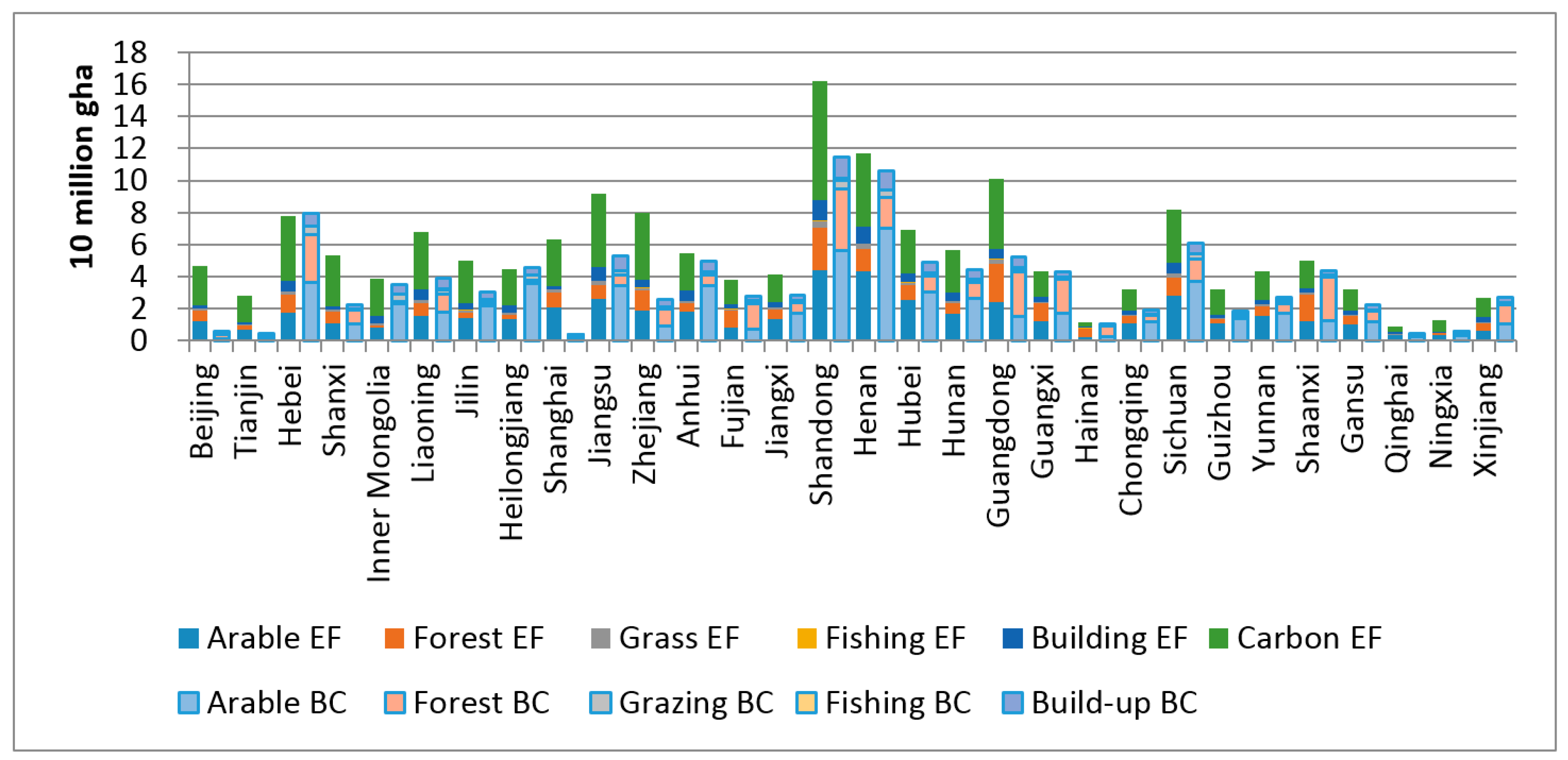
As shown in Figure 4, significant differences are observed among the values for the 30 provincial EFs in China in 2007. The EFs of Shandong, Henan, Guangdong and Jiangsu are the four highest regions, reaching 162 million, 117 million, 101 million and 92 million gha, respectively, and accounting for 9.78%, 7.06%, 6.12% and 5.52% of all national EFs, respectively. These four provinces have large populations and specific driving factors: Shandong is an energy-based province; Henan is China’s grain production base; and Guangdong and Jiangsu have well-developed industries. It is worth noting that Qinghai is the smallest province in terms of EF with 8.86 million gha, which is only 5% of Shandong’s EF. This result is mainly related to the reduced development of Qinghai, Ningxia, Xinjiang and Gansu regions and their small economic scales, minimal industrial structures and low per capita consumption levels. Because of the small populations, the EFs of Hainan and Tianjin are also relatively small. In Beijing, the total EFs are among the highest of the municipalities of Shanghai; although the population is relatively small, the high per capita consumption level is high.

Moreover, the BCs of Shandong and Henan, at more than 100 million gha, are ranked as the top two in China and account for 10.42% and 9.62% of the national BC, and these BC values are larger than the EF proportions. However, the BCs of Guangzhou and Jiangsu only account for 4.77% and 4.82% of the national BC, and these values are less than the EF proportion. The non-equilibrium of regional ecological resources involves significant differences in ecological deficits.

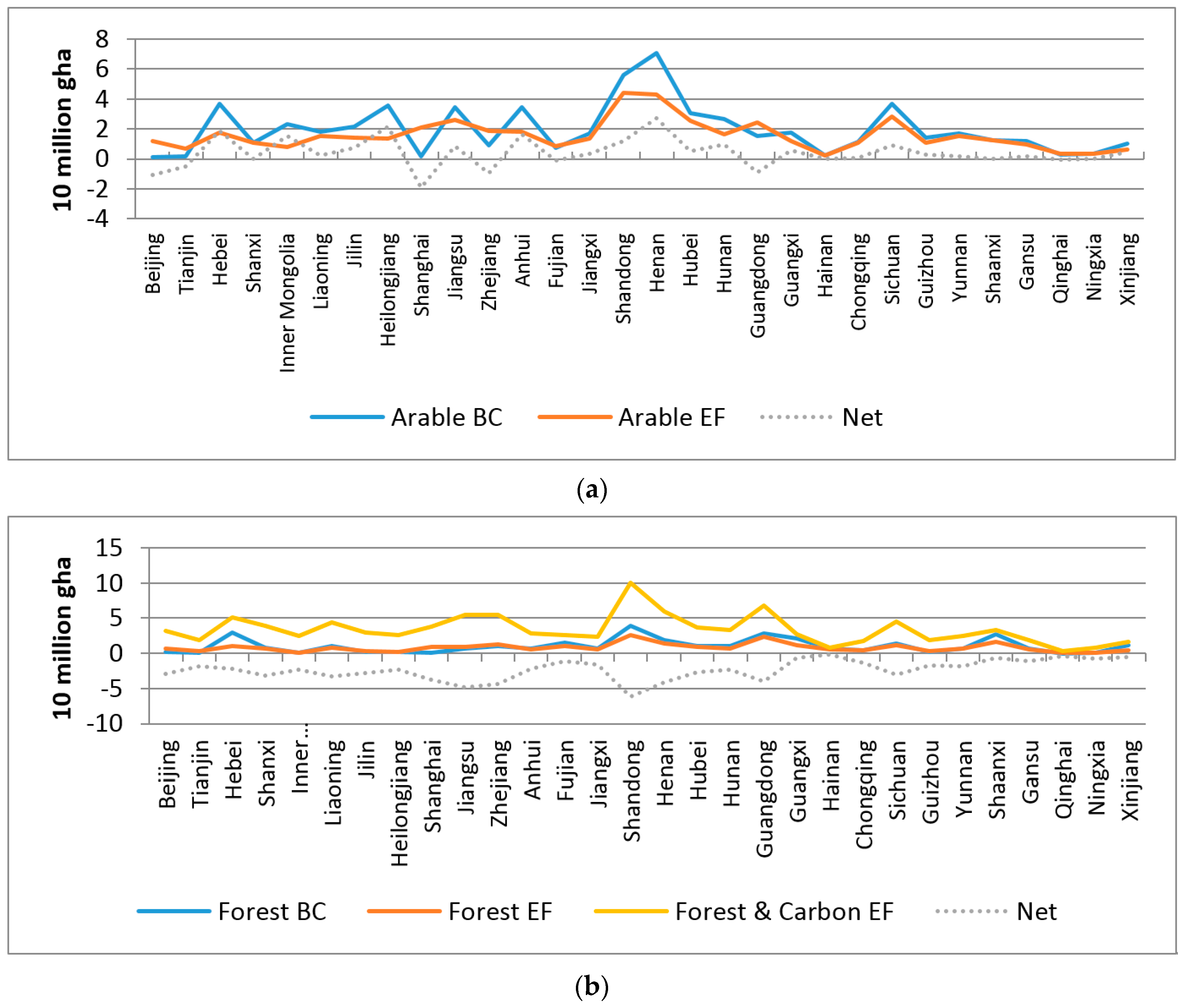
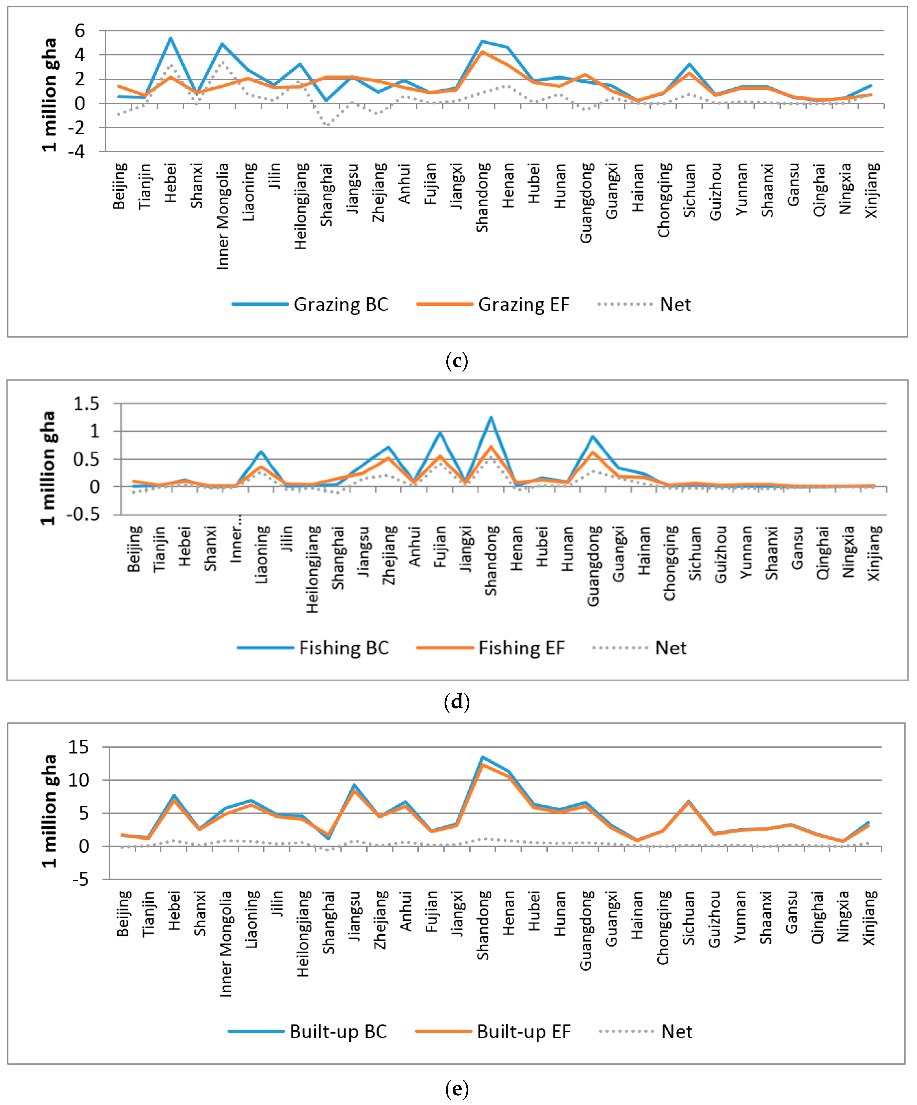
According to the footprint types, most of the blue line shown in Figure 5a is below the orange line, which indicates that the overall sustainability of arable land is relatively improved. Provinces with EF > BC are mainly divided into two categories. Beijing, Tianjin, Shanghai, Zhejiang, Fujian and Guangdong represent economically developed provinces in which the proportion of agricultural land is decreasing because of industrialization and the population is relatively large because of migration. According to natural endowments, the arable lands of other regions, such as Shanxi and Qinghai, are relatively small, and these regions also show ecological deficits. Figure 5b shows that the forest BC are necessitated by the production of forest products and carbon up-take, which require a significant amount of forest resources. In 2007, the ecological resource of all 30 provinces showed deficits, and the largest ecological deficit (ED) was observed in Shandong Province at 61.71 million gha, followed by Jiangsu, Zhejiang, Henan and Guangdong, which had EDs of 48.02, 43.88, 40.65 and 39.86 million gha, respectively.

Figure 5c provides a provincial comparison of the grazing lands of the eight provinces that showed deficits in 2007 (Beijing, Shanxi, Shanghai, Zhejiang, Guangdong, Chongqing, Gansu and Qinghai). These deficits were much smaller than those of forests and arable lands because of the reduced demand for grassland products in China. Figure 5d compares the fishery resources and shows that most of the provinces are in a state of EF > BC, which is sustainable. Moreover, surpluses are observed in certain coastal provinces, such as Liaoning, Jiangsu, Zhenjiang, Shandong and Guangdong. The dotted line in Figure 5e is almost straight, indicating that the built-up ED of the 30 provinces is small.

4.1.2. Per Capita EF, Per Capita BC, EPC and EPP for Each Province

Each provincial per capita EF reflects the local consumption level of final use, and this value is useful for analyses based on personal consumption. Figure 6 demonstrates the differences between the total amounts of EF and BC per capita for each province. Overall, the EFs of 30 provinces except Guangxi, Hebei, Heilongjiang and Xinjian are in a state of ecological deficit. Shanghai, Beijing and Tianjin, which represent three of China’s four municipalities with high population densities and personal consumption levels (3.03, 2.91 and 1.85 ten thousand yuan, respectively), present the most serious ecological deficits.

We employ the indicator EPC, which is calculated by Formula (4), as an intuitive method of expressing the sustainable state of the local environment. The EPC values of the 30 provinces are divided into four levels. As shown in

Table 5. Ecological pressures in consumption (EPCs) for the province and the arable, forest, grazing, fishing and built-up land for each province of China in 2007.

Rate	Ranking	Province	EPC	Arable EPC	Forest EPC	Grazing EPC	Fishing EPC	Built-Up EPC
I	1	Heilongjiang	0.98	0.39	11.93	0.41	2.58	0.88
	2	Hebei	0.98	0.48	1.73	0.40	0.77	0.89
	3	Xinjiang	0.98	0.59	1.42	0.48	5.36	0.87
	4	Guangxi	1.00	0.68	1.32	0.69	0.54	0.89
II	5	Hainan	1.08	0.95	1.16	0.91	0.78	0.89
	6	Anhui	1.09	0.53	4.45	0.69	0.93	0.90
	7	Henan	1.11	0.61	3.10	0.69	3.44	0.93
	8	Inner Mongolia	1.11	0.34	20.39	0.29	3.93	0.85
	9	Shaanxi	1.15	1.00	1.24	0.93	18.12	1.01
	10	Hunan	1.29	0.63	3.39	0.65	0.89	0.92
	11	Sichuan	1.34	0.76	3.24	0.76	1.50	0.98
	12	Fujian	1.40	1.11	1.68	1.00	0.56	0.93
	13	Shandong	1.41	0.79	2.59	0.83	0.58	0.91
	14	Hubei	1.42	0.83	3.70	0.96	0.84	0.91
	15	Gansu	1.44	0.84	2.76	1.04	22.00	0.95
	16	Jiangxi	1.44	0.80	3.41	0.87	0.89	0.92
	17	Yunnan	1.60	0.90	3.90	0.92	3.43	0.93
	18	Jilin	1.65	0.66	12.60	0.86	7.22	0.93
	19	Chongqing	1.68	0.93	4.19	1.02	3.64	1.00
	20	Jiangsu	1.73	0.76	8.26	0.96	0.61	0.90
	21	Liaoning	1.73	0.86	4.02	0.75	0.57	0.90
	22	Guizhou	1.74	0.78	9.89	0.95	6.87	0.95
	23	Qinghai	1.86	1.23	83.64	1.24	33.00	0.97
	24	Guangdong	1.93	1.61	2.42	1.32	0.69	0.91
III	25	Ningxia	2.22	0.99	6.82	0.91	2.66	1.00
	26	Shanxi	2.40	1.01	4.86	1.13	15.37	0.95
	27	Zhejiang	3.08	2.01	5.18	1.97	0.71	0.98
IV	28	Tianjin	6.59	4.35	22.01	1.32	1.57	0.92
	29	Beijing	7.81	8.99	12.56	2.72	24.57	1.08
	30	Shanghai	15.16	13.87	30.19	9.67	3.80	1.51

, the provinces in level I (EPC ≤ 1) are Heilongjiang, Hebei, Xinjiang and Guangxi, which reflects sustainable development that is close to the threshold; and the per capita BCs of these four provinces are 1.19, 1.14, 1.31 and 0.91 gha, respectively, which exceeds the national average of 0.84, whereas the per capita EFs are 1.17, 1.12, 1.29 and 0.91 gha, respectively, which are close to or below the national average EF per capita of 1.27. Therefore, the ecological sustainable development of the four provinces would benefit from good natural endowments, a reasonable population size, and a reasonable level of ecological consumption.

For 20 provinces, the EPCs are between 1 and 2 and the EDs are no higher than the regional corresponding BC; thus, these provinces are placed into level II. The sub-indexes of EPC are obviously different among the provinces. Arable EPCs that exceeded 1 are observed in Guangdong, Qinghai and Fujian at values of 1.61, 1.23 and 1.11, respectively. The per capita arable BC for Guangdong and Fujian is small, and the arable EFs per capita are 0.25 and 0.23, respectively, which is much lower than the national average of 0.36. Qinghai is a special example with an extremely small population and minimal consumption structure. Because of the need for more forests for the absorption of CO₂, each province in level II exceeds the threshold value for forest EPC, and the most serious cases are in Qinghai, Inner Mongolia and Jilin at values of 83.64, 20.39 and 12.60, respectively. Grazing EPCs are relatively smooth, and only the EPCs of Guangdong, Qinghai, Gansu and Chongqing are excessive at values of 1.32, 1.24, 1.04, and 1.02, respectively. Because of the significant differences between the provinces with regard to fishing resources, the differentiation of per capita fishing BC is significant, which can be explained by the rich fishing resources and higher fishing BC per capita of the coastal provinces, including Hainan, Fujian, Shandong, Jiangsu, Liaoning and Guangdong, all of which have fishing EPCs of less than 1. Inland provinces such as Hubei, Anhui, Hunan, and Jiangxi, which have rich inland lakes, are still in a state of sustainable development. Provinces in the western and other arid regions with fewer fishing resources are as follows (in descending order): Qinghai, Gansu, Shaanxi, Jilin, Guizhou, Inner Mongolia, Chongqing, Henan, Yunnan, and Sichuan. For the built-up EPC, the provinces are in a state of sustainable development except for Shaanxi, which has a slightly excessive value of 1.01.

Ningxia, Shanxi and Zhejiang are in level III and have EPCs between 2 and 5, and their per capita EFs are 2.11, 1.58 and 1.55 gha, respectively, which exceed the national average value. The BC per capita of Shanxi and Zhejiang is far below the national average, and the Ningxia BC is only slightly higher than the national average.

These results show that Shanghai, Beijing and Tianjin are municipalities with large population densities, large ecological carrying capacities, and EF gaps. As shown in Table 5, the EPC is 15.09, 8.45 and 6.31 and the sub-pressure indexes for arable, forest, grazing, fishing and built-up land are greater than 1 except for the built-up EPC of Tianjin, which represents severe ecological sustainability at level IV.

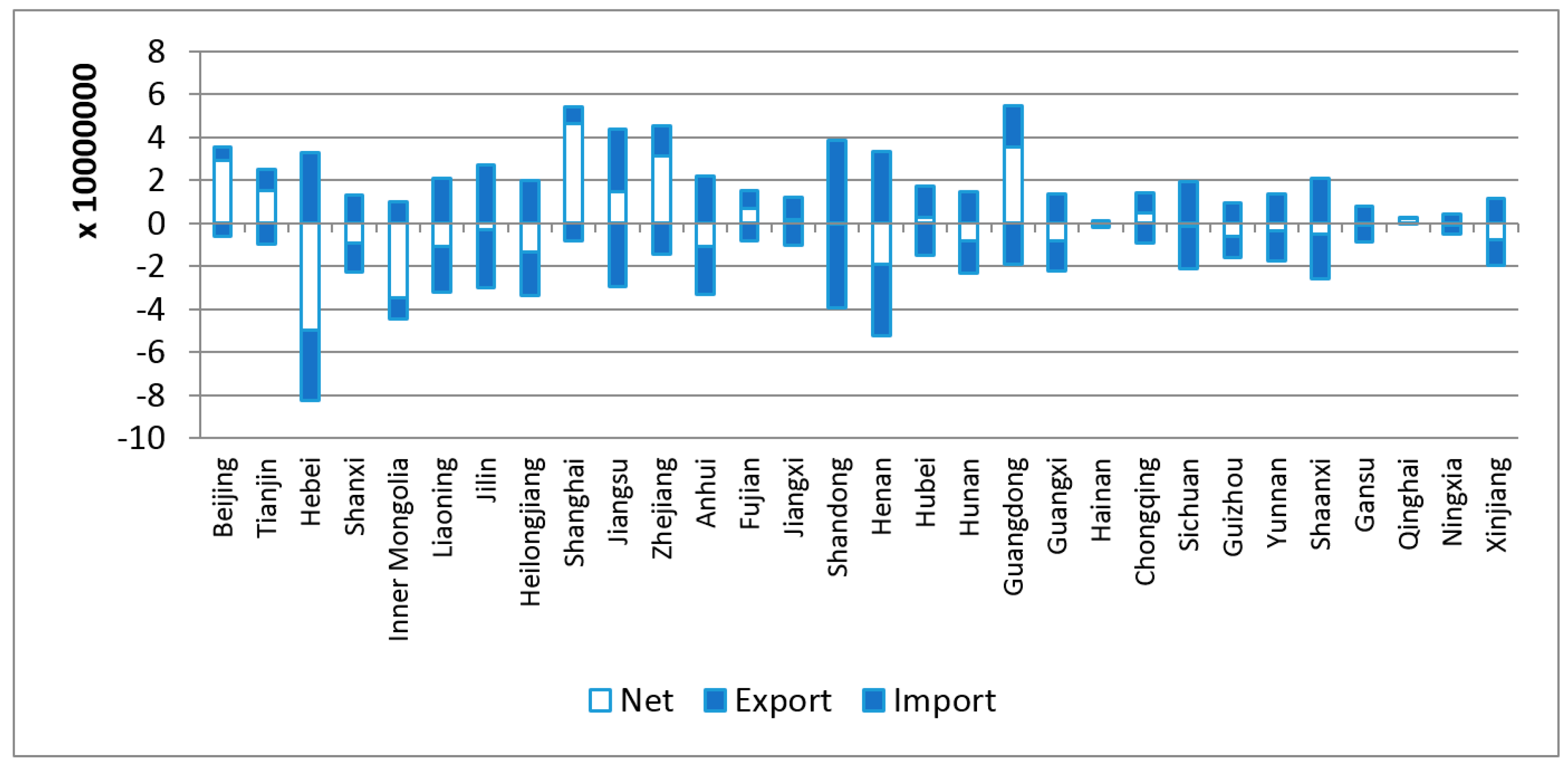
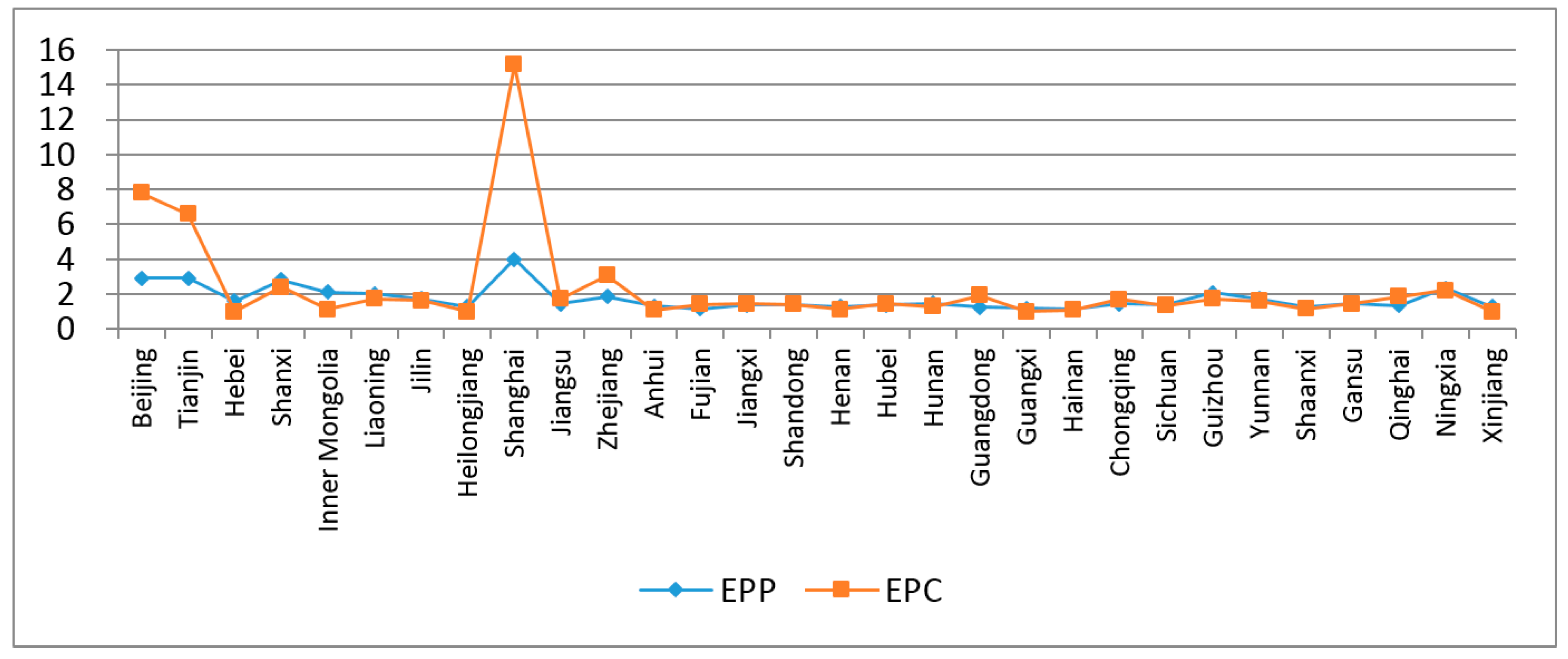
The EPC reflects the number of years that a local BC must support domestic consumption, which is a type of pressure in consumption; however, the local ecological pressure in production (EPP), which expresses the local realities of EP, must be determined, and it is calculated according to the EF of local production divided by the local BC. The gap between the two indicators of the region is mainly caused by the embodied EF flow.

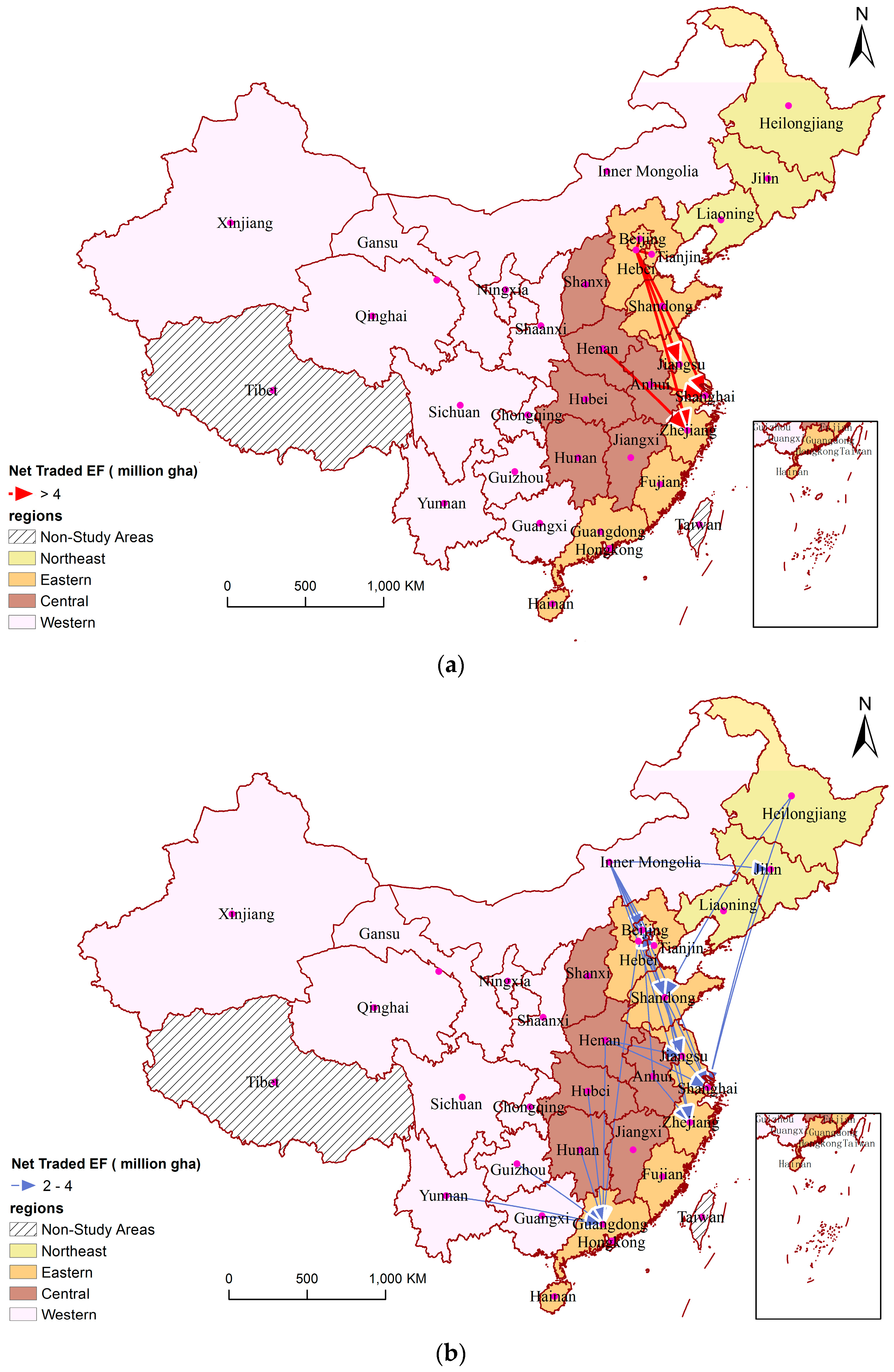
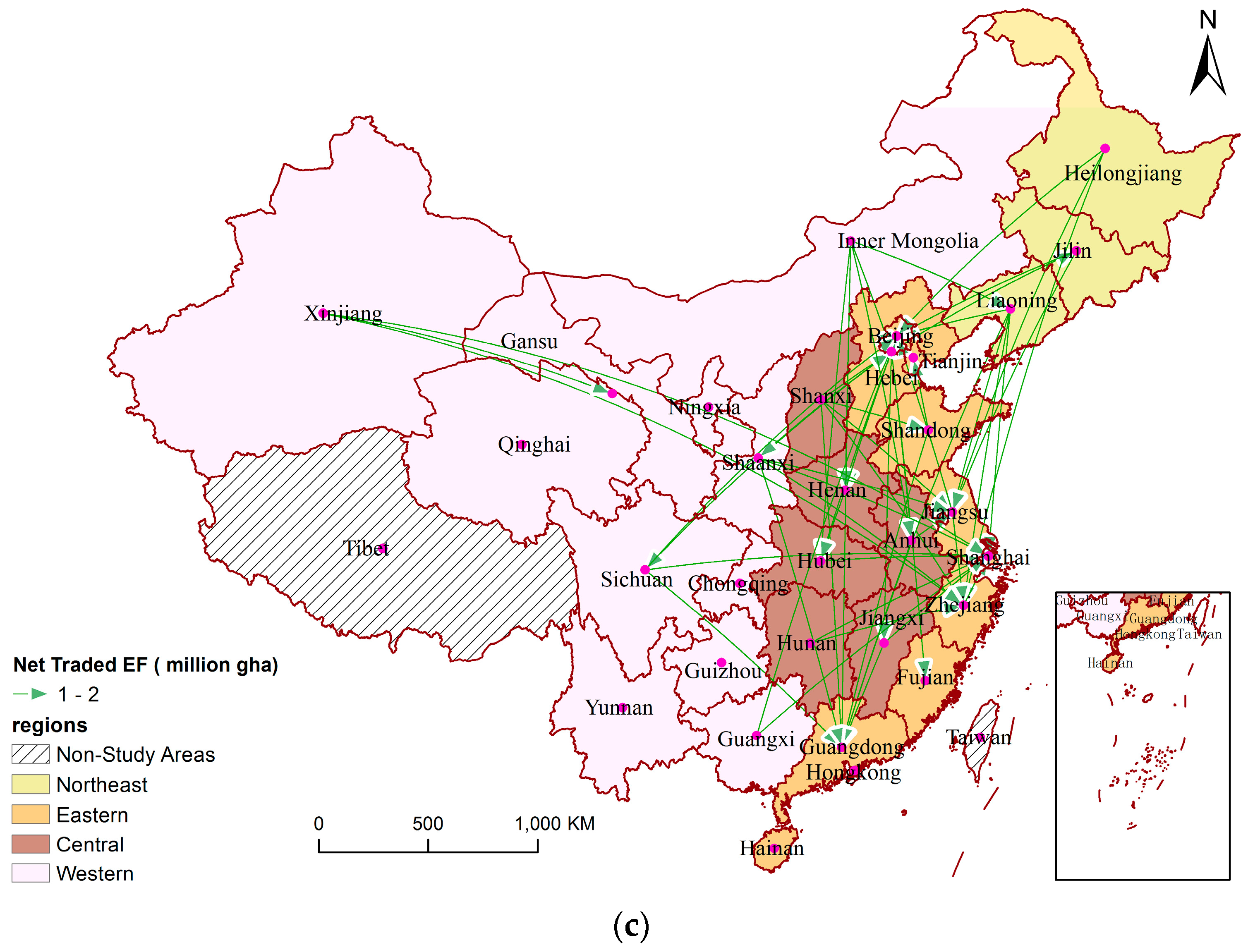
As shown in Figure 7, both the EPC and EPP of the 30 provinces are larger than 1 except the EPC of Heilongjiang, Hebei, Xinjiang and Xinjiang, which means that regardless of the EPC or EPP, ecological sustainability issues in China were serious in 2007. A reduction of the embodied EFs is necessary to reduce the stress from a consumption perspective; however, the pressure from production should not be ignored. Provinces such as Heilongjiang, Hebei, Xinjiang and Guangxi have had sufficient BC to support local consumption because of the exports of embodied EFs in the form of industry shifts, and the actual utilization of the ecological resources is beyond that of the local BCs. However, the EPCs of Shanghai, Beijing, Tianjin and Zhejiang are all much larger than their corresponding EPPs because embodied EFs are imported. To achieve an interregional ecological balance, the local industrial structure, consumption levels, and ecological balance estimates should be studied to determine the EF intensity by total EF and sector, and the embodied EF flows among the regions according to the total EF, EF type and sector will be studied in the following sections.

4.2. Sector Analysis of EF Intensity

An analysis of the total and sectoral EF intensity of China’s provinces can identify the industries that constrain regional ecologically sustainable development and produce more refined questions. Overall, the EF is primarily generated by the agriculture, industry and construction sectors, whereas the other services, transportation, and wholesale and retail trade sections contribute a lower proportion. Because of the different industrial structures of each region, the proportion of regional EF is different between the provinces in each sector (Figure 8), and so is the direct consumption of the carbon footprint and built-up footprint. The prominent EF sector types vary. For example, the arable EF proportions of Hainan, Shaanxi, Yunnan, Gansu, Qinghai, Guangxi, Guizhou, Chongqing, Sichuan, Jiangxi and Xinjiang, which are all mid-western provinces, are the largest, whereas the industry sector is the largest EF type of the remaining 17 provinces. Because the 30 provinces differ greatly in provincial productivity and eco-efficiency, the high proportion of EF does not denote a high proportion of GDP in the same sector (Figure 9), and obvious differences are observed among the different provinces and sectors.

As shown in

Table 6. China’s provincial ecological footprint intensity (EFI) and sectoral EFIs of agriculture, industry, construction, transportation, and other for each province by region.

Regions	Province	EFI	Agriculture EFI	Industry EFI	Construction EFI	Transportation EFI	Sell EFI	Other EFI
Northeast	Liaoning	0.61	1.38	0.37	1.91	0.41	0.12	0.41
	Jilin	0.95	1.36	0.74	2.39	0.91	0.37	0.54
	Heilongjiang	0.63	0.95	0.35	2.88	0.39	0.19	0.41
Eastern	Beijing	0.5	9.58	0.66	2.24	0.06	0.02	0.19
	Tianjin	0.55	2.88	0.51	3.07	0.11	0.09	0.18
	Hebei	0.57	0.75	0.39	2.17	0.21	0.13	0.4
	Shanghai	0.52	21.51	0.47	1.8	0.14	0.03	0.13
	Jiangsu	0.36	0.74	0.3	1.4	0.14	0.05	0.16
	Zhejiang	0.42	1.49	0.31	1.97	0.17	0.04	0.18
	Fujian	0.41	1.09	0.32	1	0.08	0.06	0.25
	Shandong	0.62	0.49	0.65	1.91	0.23	0.08	0.35
	Guangdong	0.33	1.77	0.21	1.49	0.15	0.04	0.15
	Hainan	0.92	1.79	0.44	1.94	0.44	0.03	0.28
Central	Shanxi	0.94	4.36	0.56	4.9	0.09	0.24	0.37
	Anhui	0.74	1.11	0.57	1.63	0.32	0.07	0.42
	Jiangxi	0.75	1.38	0.54	1.46	0.27	0.27	0.3
	Henan	0.78	1.18	0.7	1.46	0.14	0.03	0.45
	Hubei	0.75	1.34	0.79	1.82	0.32	0.11	0.2
	Hunan	0.62	0.96	0.49	1.54	0.42	0.15	0.29
Western	Inner Mongolia	0.64	0.55	0.42	2.5	0.17	0.23	0.41
	Guangxi	0.73	1.37	0.52	2	0.35	0.05	0.31
	Chongqing	0.78	2.35	0.5	1.66	0.49	0.06	0.31
	Sichuan	0.78	1.24	0.6	1.83	0.31	0.21	0.33
	Guizhou	1.17	2.68	0.64	3.12	0.46	0.37	0.43
	Yunnan	0.92	2.33	0.52	2.25	0.09	0.03	0.34
	Shaanxi	0.91	4.02	0.47	1.53	0.32	0.08	0.24
	Gansu	1.18	3.38	0.57	2.63	0.27	0.1	0.32
	Qinghai	1.13	4.35	0.36	1.38	1.19	0.46	0.28
	Ningxia	1.45	3.57	1.08	3.63	0.55	0.04	0.61
	Xinjiang	0.76	1.11	0.39	2.69	0.49	0.08	0.4

, the lowest EFI is in the eastern region, which is followed by the northeast, central and western regions. This order is inconsistent with the regions’ corresponding economic conditions. The provinces with low EFI are Guangdong (0.33), Jiangsu (0.36), Fujian (0.41), Zhejiang (0.42), Beijing (0.50), Shanghai (0.52), and Tianjin (0.55), all of which are developed provinces in the eastern region, and the provinces with high EFI are Qinghai (1.13), Guizhou (1.17), Gansu (1.18) and Ningxia (1.45), and these values are more than twice the values of the developed provinces.

An overview of the sectoral decomposed indexes indicates that the sectoral EFI of agriculture is relatively high for each region; the sectoral EFI of construction as a labor-intensive sector is at a medium level and higher than the regional EFI; and the sectoral EFI of transport, wholesale and retail and other services is relatively small. Because of the differences in the internal structure of the different industries, the level of productivity, and the energy structure, the sectoral EPIs vary among the provinces. In the tertiary sector (transportation, sales and other), the EPIs of the eastern provinces are significantly lower than those of the mid-western and northeastern provinces. In the eastern region, Shanghai, Guangdong, Jiangsu, Tianjin, Zhejiang, Beijing and Fujian present low tertiary sectoral EFIs of 0.12, 0.13, 0.13, 0.13, 0.15, 0.16, and 0.18, respectively, whereas in the mid-western and northeastern regions, Liaoning (0.33), Anhui (0.34), Heilongjiang (0.36), Xinjiang (0.36), Guizhou (0.43), Qinghai (0.44), Ningxia (0.52) and Jilin (0.55) present higher tertiary sectoral EFIs.

The significant differences among the regions can be explained by the transfer of EF-intensive industries from developed provinces to less-developed provinces. This transfer results in a decline of the EFI of industrial transfer exporters and an increase in the EFI of industrial transfer importers. For industrial transferals, the importation of carbon-intensive industries from eastern regions according to the GDP, employment rates, etc. and the lower productivity of energy industry equipment in mid-western provinces causes the industrial EFIs of the mid-western provinces to be significantly higher than those of the eastern provinces [40].

4.3. EF Flow of Interregional Trade

4.3.1. Import, Export and Net EF Traffic for Each Province and Region

Here, “import” (“export”) means the import (export) of ecological resources as measured by embodied EFs to (from) the local region from (to) the external regions within China as shown below [47]. Embodied EF flows among the regions reveal regional connection degrees, and the net value reveals the regional ecological equities among the provinces. The interprovincial and interregional EF flows by EF type will be analyzed to reveal the deeper implications.

Figure 10 presents the embodied EFs related to exports, imports and net flows for each province from the viewpoint of consumption. The positive values in blue indicate the EF imports from the external provinces, and the negative values in blue indicate EF exports to external provinces. The value of the empty column represents the provincial net embodied EFs. The largest net embodied EF importer is Shanghai at a value of 46.50 million gha, followed by Guangdong, Zhejiang, Beijing and Tianjin at values of 35.71, 31.39, 29.40 and 15.50 million gha, respectively, and these values represent more than 38% of the responding regional EFs. The large net embodied EF imports from those provinces were based on the developed economies, a scarcity of natural resources, and the high population and per capita consumption. The largest net embodied EF exporters are Hebei, Inner Mongolia, Henan, Heilongjiang and Liaoning at values of 49.47, 34.44, 18.86, 13.35 and 10.86 million gha, respectively, and this result is related to the large agriculture product exports from Henan and the large energy exports from the remaining four provinces. However, the total length of the column represents the total flows for a province, the size of which implies a connection degree with other provinces that indirectly reflects the level of the local economy. The larger provinces are followed by Hebei (8.76% of the national total), Henan (6.48%), Shandong (5.89%), Guangdong (5.63%), Jiangsu (5.56%), Shanghai (4.72%), and Zhejiang (4.52%), and the EF flow of these seven provinces account for more than 50% of all of China’s EF traffic.

Figure 11 shows the embodied EF traffic of China’s four regions in 2007. Only the eastern region is a net importer of embodied EFs, whereas the northeast, southwest and central regions are net exporters. As demonstrated by the sizes of the column values, which indicate the regional embodied EF traffic, the eastern, northeast, central and western regions account for 41.41%, 14.03%, 19.37% and 25.19%, respectively, which verifies the corresponding proportion of national GDP. The embodied EF traffic of the eastern region is significantly greater than that of the other regions, which can be explained by the active economic and population aggregation in the eastern region. However, the development of the eastern region has occurred at the ecological expense of the northeast, southwest and central regions. To balance and harmonize the development among the regions, we must study interregional flows as well as interprovincial flows.

4.3.2. Net EF Flow from Province to Province and Region to Region

Although the traffic and total net flows of each province and region were studied in the previous section, the details of the net flows among the provinces and regions were not clarified. Formula (24) can calculate the total, sectoral or categorized net EF flows among the provinces and regions. There are 435 provincial net EF flows among the 30 provinces, although this study only focuses on flows with net embodied EFs of more than one million gha.

The calculations indicated that China’s net embodied EF flows in 2007 presented three main characteristics.

(1) Spatial Aggregation

Spatial aggregation is mainly reflected in two aspects: the export and import of spatial aggregation. As shown in Figure 12, the arrowed line represents the net embodied EF flow, with the province at the starting point exporting embodied EFs directly or indirectly in the form of production or services to the end point.

Regions with high densities of arrowed lines are mainly concentrated in the eastern, northeastern and central regions of China, indicating that one of the connections between the eastern, northeastern and central regions is closer than that between the western region and the other regions. The spatial aggregation of the end points indicates the five provinces with the largest number of connections (in descending order): Shanghai (17), Guangdong (15), Zhejiang (12), Beijing (11), and Jiangsu (10). All of these provinces are developed provinces in eastern China, and they have external EFs that accounted for 66.16%, 30.65%, 34.04%, 48.66% and 20.32% of the corresponding local EFs.

However, the starting point provinces (Figure 13) indicate that the EPPs are transported to the end point provinces concurrently with the import of the embodied EFs. The five provinces with the largest number of connections (in descending order) are Inner Mongolia (15), Hebei (9), Shanxi (9), Guizhou (7) and Xinjiang (7), which have external EPPs of 0.85, 0.50, 0.42, 0.34 and 0.26, respectively. These provinces are energy-based provinces that operate at the expense of environmental pollution, and increased EPPs are required to drive local economies. Regardless of the starting or ending point, points located closer to these geographical centers present larger embodied EF trades.

(2) Different EPP and Net Embodied EF Flow Levels

Figure 12 shows the three levels of net embodied EF flows. The large flows (Figure 12a) indicated in red (accounting for more than 4 million gha) are from Hebei to Shanghai, Beijing, Zhenjiang and Jiangsu; from Henan to Zhejiang; and from Hebei to Tianjin and Anhui. A total of 27 flows indicated in violet (Figure 12b) are at the middle level and mainly flow from the mid-western provinces to Shanghai and Guangdong, and they have EFs between 2 and 4 million gha. The left flows indicated in green (Figure 12c) represent between 1 and 2 million gha and are considered low-level flows. Because of the limited space, the flow details at the middle and low levels are not listed. In addition, we can calculate the EPPs of the net embodied EFs that refer to the exporter’s BCs. The EPP from Guangdong to Guizhou is up to 0.15, which is the largest, whereas the net embodied EF flow between them in the opposite direction is only ranked 15th. The significant differences between the orders are assessed according to an EPP analysis.

As demonstrated in Figure 13, the EPPs of the flows are also divided into three levels. The large level includes 18 EPPs with flows that are indicated in red (Figure 13a), and they are mainly moving to Guizhou, Inner Mongolia and Yunnan (less BC) and to Hebei, Anhui and Shanxi (large net embodied EF imports), which result in relatively significant EP on the EF exporters. The middle level includes a total number of 59 EPPs with flows that are indicated in violet (Figure 13b), and they are mainly brought from eastern provinces to the central and western provinces and from the central provinces to the western provinces, which results in a moderate level of EP on the EF exporters. The low level includes 35 EPPs with flows that are indicated in green (Figure 13c), and they move between two provinces that are far from each other, which results in low EP on the EF exporters. Both the net embodied EFs and EPPs of the flows are necessary to identify a reasonable method of achieving interregional ecological balance.

(3) Different Industries and Types of EFs

In the trade of embodied EF and based on the various types of EFs, arable and carbon footprints are the main EF types whereas the main sector is the primary sector followed by the secondary sector. Because of the complicated geographical factors, we investigated the sectors and categorized the EFs based on the division of the four regions.

Table 7. Flows of the total embodied net EFs in China’s four regions in 2007 (1 million gha).

	Northeast	Eastern	Central	Western
Northeast	101.22	23.49	5.32	0.00
Eastern	0.00	410.46	0.00	0.00
Central	0.00	49.31	262.98	0.00
Western	1.79	57.31	1.56	274.12

shows the EF flows of four regions in China, and the results are as follows: the eastern region is a net embodied EF importer, the western region is a net EF exporter; and the northeastern region is a net exporter to the central region.

Table 8. Embodied net flow of arable, forest, grazing, fishing, built-up and carbon EFs in China’s four economic regions in 2007 (1 million gha).

		Northeast	Eastern	Central	Western
Arable EF	Northeast	32.23	14.22	1.95	0.20
	Eastern	0.00	98.00	0.00	0.00
	Central	0.00	26.76	104.03	3.87
	Western	0.00	20.10	0.00	94.91
Forest EF	Northeast	8.04	0.00	0.00	0.00
	Eastern	0.47	86.68	0.00	0.00
	Central	0.12	3.72	34.85	0.00
	Western	0.67	10.19	2.63	55.18
Grazing EF	Northeast	3.42	1.18	0.29	0.00
	Eastern	0.00	10.49	0.00	0.00
	Central	0.00	1.28	6.94	0.00
	Western	0.18	2.53	0.24	8.74
Fishing EF	Northeast	0.38	0.03	0.02	0.02
	Eastern	0.00	2.94	0.08	0.09
	Central	0.00	0.00	0.26	0.01
	Western	0.00	0.00	0.00	0.25
Built-up EF	Northeast	2.30	0.51	0.10	0.01
	Eastern	0.00	7.49	0.00	0.00
	Central	0.00	1.05	5.75	0.17
	Western	0.00	0.79	0.00	4.63
Carbon EF	Northeast	54.85	8.01	3.08	0.00
	Eastern	0.00	204.87	0.00	0.00
	Central	0.00	16.60	111.16	0.00
	Western	1.18	23.79	2.74	110.43

shows China’s regional net embodied footprint flows of arable, forest, grazing, fishing, built-up land and carbon in 2007. Because of the large proportion (71%) of the directly built-up EF, the flows of the built-up embodied EF are small, whereas the main flows among the four regions are arable and carbon EFs, which represent 45.07% and 37.21%, respectively, of the national net embodied EF traffic. For the net flows of embodied arable EFs, the eastern region imports the most because of its dense population, less per capita arable land, and regional functions, such as Henan and Anhui in the central region, which are food production bases. The main flows of the carbon footprint are caused by an increasing amount of carbon-intensive industries migrated from the eastern to central and western regions, and clean materials and processed energy are imported to the eastern region with less CO₂ emissions in use again. For forest and fishing land, the flows result from unbalanced distributions of specific natural endowments. The main embodied grazing footprints exported from the northeast and western regions and the main footprints embodied in the fishing footprint exported from eastern region can be explained by the location of most of China’s grazing lands, which are in the western area of the northeast region, Inner Mongolia, and the northwest area of the western region, and the location of China’s rich fishing resources, which is in the eastern region by the sea.

Table 9. Four net embodied EF flows of the primary, secondary, and tertiary sectors in China’s four economic regions in 2007 (unit: 1 million gha).

		Northeast	Eastern	Central	Western
Primary Sector	Northeast	46.11	15.79	2.31	0.00
	Eastern	0.00	205.12	0.00	0.00
	Central	0.00	32.77	151.26	1.14
	Western	0.59	33.71	0.00	163.82
Secondary Sector	Northeast	46.32	7.31	2.85	0.00
	Eastern	0.00	181.47	0.00	0.00
	Central	0.00	16.08	99.31	0.00
	Western	1.09	21.48	2.22	93.96
Tertiary Sector	Northeast	8.79	0.39	0.16	0.00
	Eastern	0.00	23.87	0.00	0.00
	Central	0.00	0.46	12.41	0.00
	Western	0.12	2.12	0.48	16.34

presents the sectoral flows of embodied EFs. On a national scale, the three sectors represent 47.91%, 48.19% and 3.9% of the national net traffic of embodied EF, whereas the GDP of the three sectors is 10.36%, 50.22% and 39.42%. The main embodied EFs of the flows are from the primary and secondary sectors. Although the economic benefits of the primary sector are low, EFs must be traded because of the fundamental nature of food. The ability to lower the embodied EF of a region, which introduces additional EPP, is observed in the secondary sector. However, for the tertiary sector, the proportion of the national net traffic for the embodied EFs is especially small compared with the proportion of the national GDP, indicating that the development of this sector, especially for less developed regions, is beneficial for lowering the net embodied EF imports and achieving local ecological sustainability. Table 8 and Table 9 indicate that the amount of the secondary sectoral net embodied flow between two regions is close to that of the corresponding net embodied carbon footprint flow, indicating that the main EF type of the secondary sectoral EF trade is the carbon footprint.

5. Discussion and Conclusions

5.1. Ecological Issues

This study investigated the total provincial EFs and BCs and revealed that China’s provincial BC showed major deficits in 2007 that are mainly concentrated in forest and arable BC. The geographical distributions were not balanced, with major deficits observed in most eastern and northeastern provinces and small or no deficits observed in central and western provinces. Obvious differences were observed in the provincial per capita EFs among the provinces, with Beijing, Shanghai and Tianjin, which represent developed municipalities, facing high consumption issues. To reflect the degree of ecological consumption, we used EPC and EPP as the EPs in consumption and production, respectively. Only four provinces were in a sustainable state of potentiality, whereas none of the provinces had EPP values less than one. Moreover, the EPC and EPP values indicated that the sustainable states of Hainan and Guangxi are relatively good.

The EFI was used to analyze “hot spots” of EFs among the provinces and sectors. The results showed that for the provincial data in general, the EFIs of the eastern provinces were significantly lower than those of the central and western provinces, and the same trend was also observed for the industrial EFIs among the regions, although the results were not significant. The tertiary sector had much larger proportions in the eastern provinces than in the central and western provinces, which indicated that the disparity of provincial EFIs resulted in obsolete equipment and technology and an unsustainable industrial structure.

The net embodied EF flows among the provinces and regions indicated that the eastern region is the only net importer. The main flows were also centered in the western and central provinces and flowed to the eastern provinces as a result of the developing EF-intensive industries that have migrated from the western provinces. Overall, Shanghai (17), Guangdong (15), Zhejiang (12), Beijing (11), and Jiangsu (10) exploited most of the net embodied EFs imported from other regional provinces, whereas Inner Mongolia (15), Hebei (9), Shanxi (9), Guizhou (7) and Xinjiang (7), as the energy-based provinces, were subject to negative environmental impacts with regard to the interprovincial ecological balance. In addition, Guizhou, Inner Mongolia, Yunnan, Hebei, Anhui and Shanxi exported the largest proportion of corresponding BC in a single EF flow from the perspective of EPP, which can be used to determine provincial ecological compensation from point to point. The sectoral and categorized net embodied EF flows indicated that the imbalanced carbon footprint flows in the secondary sector (except for the arable land products and imbalanced natural endowments of grazing land and finishing areas) among the provinces and regions are of urgent concern.

Overall, there exists imbalance and inequities in terms of China’s EF and BC. Consequently, EP comes into being.

The imbalance embodies the following three aspects. The first aspect lies in province-level EF and BC and their differences. For instance, although the provincial EFs and BCs alone did not seem to be a problem, their distributions in China in 2007 were imbalanced. Therefore, what really matters is their differences, which are termed as ecological deficit or ecological surplus. In addition, these imbalances are also reflected in each land type, (arable, forest, grazing, fishing and built-up), due to the specific natural endowments of each province. For example, the eastern coastal provinces are rich in water resources, so in order to balance the ecological deficit and surplus among provinces, embodied EF flow occurs. Secondly, net embodied EF is imbalanced as well, which mainly flows to the eastern region from central, northeast and western regions. The net EF importers are cities and provinces located in the eastern region, such as Shanghai, Guangdong, Zhejiang, Beijing and Tianjin. Thirdly, due to different industry structures, the EFI of the provinces in China are imbalanced as well.

The issue of inequities is mainly reflected in two aspects. The first aspect is per capita BC and per capita EF. As a matter of fact, the major reason behind the inequity of per capita BC is population density. For example, per capita BCs are relatively small in cities like Shanghai, Tianjin and Beijing since their population density is quite high. On the contrary, per capita BCs in Xinjiang and Hainan provinces are relatively large because they have lower population density. The imbalance of per capita EF lies in the fact that the figure in economically developed provinces is significantly higher than that in the developing provinces. The other aspect is the inequity of EF flows among regions and provinces. For example, the products and services that the eastern region enjoys are normally produced in the western region with high carbon emissions and more land appropriation.

Ecological pressure exists in almost all provinces in terms of both consumption and production. Both of these two kinds of pressure deserve attention because, on one hand, production is measured by local direct carbon emission and land appropriation. On the other hand, the consumption of the externally traded EF will eventually be traced to a place. It is meaningful to study how to achieve overall ecological sustainable development in China. What is more, the ecological pressure in consumption also serves as a wake-up call to end consumers and urge them to lower EF consumption.

5.2. Policy Implications

In this study, we quantified ecological sustainable development according to two indicators to achieve an ecologically sustainable state, which was indicated by EPC and EPP values less than “1”. To achieve this goal, we propose the following suggestions.

(1) Total EF in Production Policy

For the total provincial EF, each province should use a specific strategy to decrease the embodied EF in the intermediate link of production. The EFIs of the eastern provinces are low, whereas the total EFs are large because of the large proportion of national GDP; therefore, industrial upgrading, low-EFI industry development, tertiary sector development, and low-carbon technology implementation should be performed. The northeastern provinces should eliminate their dependence on energy in economic development and promote the tertiary sector and other low-EFI industries. The EFIs of the central and western provinces are relatively high; therefore, the economic development of these provinces should focus on industrial equipment upgrading, technology migration and tertiary sector development.

(2) Consumption Policy

From the perspective of per capita BC, both the residents and the government should take action. The government should directly guide the behavior of the population towards low EFs by encouraging green travel and reducing the depletion of residential land, although the importance of embodied EFs in final uses must be emphasized. However, the government itself should practice low-EF consumption as well because their EFs also represent a large proportion of the final use.

(3) Ecological Compensation Policy among Provinces and Regions

Because of the imbalanced interprovincial net embodied EF trade and the ecological contributions from net EF exporters to importers, an ecological compensation policy should be developed to protect the environment of exporter regions and promote balanced development among the provinces. According to the principle that he who damages the ecological environment protects it, specific compensation policies (point to point) refer to the net flow in Section 4.3. These compensations could be financial or technical and they are used to promote the ecological sustainability of exporting areas. For example, as shown in Table 8, the eastern region is obliged to make ecological compensation to the other three regions in arable EF and carbon EF. The specific compensation may include proper funding for cropland protection, advanced low carbon technology and equipment.

(4) Population Policy

The eastern provinces exhibit the greatest ecological pressure related to consumption because of a lack of ecological resources and the dense population resulting from migration, whereas the southeastern, western and central provinces have experienced population migration to the eastern provinces because of fewer employment opportunities and lower salaries, less developed economies or a lack of public services. China’s central government should implement a policy of balanced development among the regions to prevent increased population migration from less-developed regions to more-developed regions and achieve more balanced per capita BCs and EPCs among the provinces. For instance, government authorities should encourage college graduates to find employment or set up business in the central region by providing subsidies. Besides, more financial support, investment opportunities and favorable policies should be in place to attract population inflow to the central and western regions.

(5) Increasing BC Policy

Maintaining and increasing BC is another important issue for ecological sustainability. The emphasis should be laid on land use types with biological productivity, namely arable land, forest land, grazing land and fishing land. Generally speaking, there are two major strategies to increase the BCs of these four land use types. One is expanding the actual area of each land use type, and the other is improving product yield per unit area by applying advanced technology without causing any harm to land sustainability. Specifically, the major solutions to increase arable BC are threefold, including land reclamation, optimized crop type allocation based on land potential productivity analysis and cultivated land production improvement with the aid of technological method. When it comes to improving forest BC, firstly, it shall be prescribed by national policy that deforestation is compensated and complemented by afforestation practice and, secondly, forest products shall be utilized in a scientific and orderly manner. As for the increase of grazing BC, it could be achieved by maximizing grazing productivity through large-scale and intensive management on one hand and by improving ecological environment in animal husbandry production on the other. Finally, by means of artificial aquaculture, natural waters could be made full use of and fishing BC could be enhanced as a result. In addition, protecting the ecological environment of waters helps to improve the yield of fishing products as well. On top of these respective solutions, it is of great significance to preserve and further increase the BCs of these four land use types altogether. For example, if the forest is not well protected, land desertification increases, bringing about a further reduction of BC. In this sense, returning farmland to forests is also an effective way to preserve and further increase BC.

5.3. Shortcomings

Although we have included as many product types as possible when calculating the EFs, a few items, such as forest products and grazing products, were not comprehensively accounted for. Compiling a MRIO table usually presents time lags of 5–6 years, and we used the latest table from 2007 and are waiting for the 2012 table to obtain more meaningful implications. Because of the uncertainties [48] of the MRIO model, the main uncertainties in our results are observed in the aggregation of sectors. Thus, future work should focus on performing more accurate calculations of the EF in the EE-MRIO model.

References

1. Peters, G.P. From production-based to consumption-based national emission inventories. Ecol. Econ. 2008, 65, 13–23. [Google Scholar] [CrossRef]
2. Rees, W.E. Ecological footprints and appropriated carrying capacity: What urban economics leaves out. Environ. Urban. 1992, 4, 121–130. [Google Scholar] [CrossRef]
3. Wackernagel, M.; Rees, W.E. Our Ecological Footprint: Reducing Human Impact on the Earth; Island and Publishing House: Gabriola, BC, Canada, 1996. [Google Scholar]
4. Chen, B.; Chen, G.Q. Modified ecological footprint accounting and analysis based on embodied exergy—A case study of the Chinese society 1981–2001. Ecol. Econ. 2007, 61, 355–376. [Google Scholar] [CrossRef]
5. Dai, J.; Chen, B. Extended exergy-based ecological accounting of China during 2000–2007. Procedia Environ. Sci. 2011, 5, 87–95. [Google Scholar] [CrossRef]
6. Chen, B.; Dai, J.; Sciubba, E. Ecological accounting for China based on extended exergy. Renew. Sustain. Energy Rev. 2014, 37, 334–347. [Google Scholar] [CrossRef]
7. Chen, B.; Chen, G.Q. Ecological footprint accounting based on emergy—A case study of the Chinese society. Ecol. Model. 2006, 198, 101–114. [Google Scholar] [CrossRef]
8. Haberl, H.; Schulz, N.B.; Plutzar, C.; Erb, K.H.; Krausmann, F.; Loibl, W.; Moser, D.; Sauberer, N.; Weisz, H.; Zechmeister, H.G.; et al. Human appropriation of net primary production and species diversity in agricultural landscapes. Agric. Ecosyst. Environ. 2004, 102, 213–218. [Google Scholar] [CrossRef]
9. Venetoulis, J.; Talberth, J. Refining the ecological footprint. Environ. Dev. Sustain. 2008, 10, 441–469. [Google Scholar] [CrossRef]
10. Siche, R.; Agostinho, F.; Ortega, E.; Net, E. Emergy Net Primary Production (ENPP) as basis for calculation of Ecological Footprint. Ecol. Indic. 2010, 10, 475–483. [Google Scholar] [CrossRef]
11. Sutton, P.C.; Anderson, S.J.; Tuttle, B.T.; Morse, L. The real wealth of nations: Mapping and monetizing the human ecological footprint. Ecol. Indic. 2012, 16, 11–22. [Google Scholar] [CrossRef]
12. Kharrazi, A.; Kraines, S.; Hoang, L.; Yarime, M. Advancing quantification methods of sustainability: A critical examination emergy, exergy, ecological footprint, and ecological information-based approaches. Ecol. Indic. 2014, 37, 81–89. [Google Scholar] [CrossRef]
13. Odum, H.T. Self-organization, transformity, and information. Science 1988, 242, 1132–1139. [Google Scholar] [CrossRef] [PubMed]
14. Zhou, X.; Imura, H. How does consumer behavior influence regional ecological footprints? An empirical analysis for Chinese regions based on the multi-region input–output model. Ecol. Econ. 2011, 71, 171–179. [Google Scholar] [CrossRef]
15. Weinzettel, J.; Steen-Olsen, K.; Hertwich, E.G.; Borucke, M.; Galli, A. Ecological footprint of nations: Comparison of process analysis, and standard and hybrid multiregional input–output analysis. Ecol. Econ. 2014, 101, 115–126. [Google Scholar] [CrossRef]
16. Wiedmann, T. A first empirical comparison of energy footprints embodied in trade—MRIO versus PLUM. Ecol. Econ. 2009, 68, 1975–1990. [Google Scholar] [CrossRef]
17. Lenzen, M.; Pade, L.-L.; Munksgaard, J. CO2 Multipliers in Multi-region Input-Output Models. Econ. Syst. Res. 2004, 16, 391–412. [Google Scholar] [CrossRef]
18. Tian, X.; Chang, M.; Lin, C.; Tanikawa, H. China’s carbon footprint: A regional perspective on the effect of transitions in consumption and production patterns. Appl. Energy 2014, 123, 19–28. [Google Scholar] [CrossRef]
19. Xie, X.; Cai, W.; Jiang, Y.; Zeng, W. Carbon footprints and embodied carbon flows analysis for China’s Eight regions: A New perspective for mitigation solutions. Sustainability 2015, 7, 10098–10114. [Google Scholar] [CrossRef]
20. Zhang, C.; Anadon, L.D. A multi-regional input–output analysis of domestic virtual water trade and provincial water footprint in China. Ecol. Econ. 2014, 100, 159–172. [Google Scholar] [CrossRef]
21. Giljum, S.; Bruckner, M.; Martinez, A. Material footprint assessment in a global input-output framework. J. Ind. Ecol. 2015, 19, 792–804. [Google Scholar] [CrossRef]
22. Wilting, H.C. Analysis of the sustainability of supply chains with a multi-regional input-output model. In Proceedings of the International Input Output Meeting on Managing the Environment, Seville, Spain, 9–11 July 2008; International Input-Output Association (IIOA): Vienna, Austria, 2008. Available online: http://www.iioa.org/conferences/intermediate-2008/pdf/6d2_Wilting.pdf (accessed on 15 August 2016). [Google Scholar]
23. Weinzettel, J.; Steen-Olsen, K.; Galli, A.; Cranston, G.; Ercin, E.; Hawkins, T.; Wiedmann, T.; Hertwich, E. Footprint Family Technical Report: Integration into MRIO Model, 2011. One Planet Economy Network. Available online: http://www.oneplaneteconomynetwork.org/resources/work-package-2.html (accessed on 15 August 2016).
24. Galli, A.; Wiedmann, T.; Ercin, E.; Knoblauch, D.; Ewing, B.; Giljum, S. Integrating ecological, carbon and water footprint into a “footprint family” of indicators: Definition and role in tracking human pressure on the planet. Ecol. Indic. 2012, 16, 100–112. [Google Scholar] [CrossRef]
25. Ewing, B.R.; Hawkins, T.R.; Wiedmann, T.O.; Galli, A.; Ertug Ercin, A.; Weinzettel, J.; Steen-Olsen, K. Integrating ecological and water footprint accounting in a multi-regional input–output framework. Ecol. Indic. 2012, 23, 1–8. [Google Scholar] [CrossRef] [Green Version]
26. Peters, G.P. Opportunities and challenges for environmental MRIO modelling: Illustrations with the GTAP database. In Proceedings of the 16th International Input-Output Conference of the International Input-Output Association, Istanbul, Turkey, 2–6 July 2007; International Input-Output Association (IIOA): Vienna, Austria, 2007. Available online: http://www.iioa.org/conferences/16th/files/Papers/Peters_LP.pdf (accessed on 15 August 2016). [Google Scholar]
27. Wiedmann, T.; Minx, J.; Barrett, J.; Wackernagel, M. Allocating ecological footprints to final consumption categories with input–output analysis. Ecol. Econ. 2006, 56, 28–48. [Google Scholar] [CrossRef]
28. Promoting the Rise of the Central Region Based on a Number of Opinions. Available online: http://www.gov.cn/zhengce/content/2012-08/31/content_1147.htm (accessed on 15 August 2016). (In Chinese)
29. Issuing a Number of Policies and Measures on the Western Development Implementation of Policies. Available online: http://www.gov.cn/gongbao/content/2001/content_60854.htm (accessed on 15 August 2016). (In Chinese)
30. Division of Central and East China and Northeast China of National Bureau of Statistics. Available online: http://www.stats.gov.cn/ztjc/zthd/sjtjr/dejtjkfr/tjkp/201106/t20110613_71947.htm (accessed on 15 August 2016). (In Chinese)
31. Liu, W.; Chen, J.; Tang, Z.; Liu, H.; Han, D. China’s 30 Provinces and Autonomous Regions in 2007: Regional Input-Output Table Compilation Theory and Practice; China Statistics Press: Beijing, China, 2012; pp. 58–225. (In Chinese)
32. Editorial Committee of China Agriculture Yearbook. China Agriculture Yearbook 2008; China Agriculture Press: Beijing, China, 2008. (In Chinese)
33. National Bureau of Statistics of the People’s Republic of China. China Statistical Yearbook 2008; China Statistics Press: Beijing, China, 2008. (In Chinese)
34. Department of Energy Statistics affiliated to National Bureau of Statistics. China Energy Statistical Yearbook 2008; China Statistics Press: Beijing, China, 2008. (In Chinese)
35. Department of Population and Employment Statistics affiliated to National Bureau of Statistics. China Population and Employment Statistics Yearbook 2008; China Statistics Press: Beijing, China, 2008. (In Chinese)
36. Liu, M.; Zhang, D.; Min, Q.; Xie, G.; Su, N. The calculation of productivity factor for ecological footprints in China: A methodological note. Ecol. Indic. 2014, 38, 124–129. [Google Scholar] [CrossRef]
37. Worl Wildlife Fund (WWF). Living Planet Report 006, 2006. WWF Global. Available online: http://wwf.panda.org/about_our_earth/all_publications/living_planet_report_timeline/lpr_2006/ (accessed on 15 August 2016).
38. A Guide of the Compilation of Provincial Greenhouse Gas Inventory for Low Carbon Development. Available online: http://qhs.ndrc.gov.cn/gzdt/201403/t20140328_604827.html (accessed on 15 August 2016). (In Chinese)
39. International Panel on Climate Change (IPCC); National Greenhous Gas Inventories Programme (IGES). Guidelines for National Greenhouse Gas Inventories. A Primer; Eggleston, H.S., Miwa, K., Srivastava, N., Tanabe, K., Eds.; Institute for Global Environmental Strategies (IGES): Hayama, Japan, 2006; Available online: http://www.ipcc-nggip.iges.or.jp/support/Primer_2006GLs.pdf (accessed on 15 August 2016).
40. Zhou, S.; Zhao, M.; Wang, C.; Li, B. Calculation of carbon dioxide emissions considering secondary energy deployment among provinces in China. China Popul. Resour. Environ. 2012, 22, 69–75. (In Chinese) [Google Scholar]
41. Chen, H.; Tian, H.; Xiao, Y.; Chen, C. The estimation and analysis of carbon emissions in the oil refining industry of China. Environ. Prot. Oil Gas Fields 2012, 22, 1–3. (In Chinese) [Google Scholar]
42. Borucke, M.; Moore, D.; Cranston, G.; Gracey, K.; Iha, K.; Larson, J.; Lazarus, E.; Morales, J.C.; Wackernagel, M.; Galli, A. Accounting for demand and supply of the biosphere’s regenerative capacity: The National footprint accounts’ underlying methodology and framework. Ecol. Indic. 2013, 24, 518–533. [Google Scholar] [CrossRef]
43. Monfreda, C.; Wackernagel, M.; Deumling, D. Establishing national natural capital accounts based on detailed ecological footprint and biological capacity assessments. Land Use Policy 2004, 21, 231–246. [Google Scholar] [CrossRef]
44. Du, J.; Wang, J.; Teng, Y.; Zhang, T. Ecological footprint and introduction of EF-NPP. China Popul. Resour. Environ. 2008, 18, 178–183. (In Chinese) [Google Scholar]
45. Niccolucci, V.; Galli, A.; Reed, A.; Neri, E.; Wackernagel, M.; Bastianoni, S. Towards a 3D National ecological footprint geography. Ecol. Model. 2011, 222, 2939–2944. [Google Scholar] [CrossRef]
46. Niccolucci, V.; Bastianoni, S.; Tiezzi, E.B.P.; Wackernagel, M.; Marchettini, N. How deep is the footprint? A 3D representation. Ecol. Model. 2009, 220, 2819–2823. [Google Scholar] [CrossRef]
47. Xie, G.; Chen, W.; Cao, S.; Lu, C.; Xiao, Y.; Zhang, C.; Li, N.; Wang, S. The outward Extension of an ecological footprint in City expansion: The Case of Beijing. Sustainability 2014, 6, 9371–9386. [Google Scholar] [CrossRef]
48. Wiedmann, T. A review of recent multi-region input–output models used for consumption-based emission and resource accounting. Ecol. Econ. 2009, 69, 211–222. [Google Scholar] [CrossRef]
Figure 1. The four economic regions of China.
Sustainability 08 01345 g001
Figure 2. Framework for calculating EFs based on the environmentally extended multi-regional input-output (EE-MRIO) model.
Sustainability 08 01345 g002
Figure 3. Illustration of an EF’s divisions.
Sustainability 08 01345 g003
Figure 4. Comparison between the EF and biocapacity (BC) of China’s provinces by land type in 2007.
Sustainability 08 01345 g004
Figure 5. Comparisons between the BC, EF and net value (deficit or surplus of BC) for each type of ecological land: (a) arable land; (b) forest land (includes the forest and carbon EF); (c) grazing land; (d) fishing area; and (e) built-up land.
Sustainability 08 01345 g005aSustainability 08 01345 g005b
Figure 6. Comparison of per capita EF and per capita BC for each province in China in 2007.
Sustainability 08 01345 g006
Figure 7. Comparison between the ecological pressure in consumption (EPC) and ecological pressure in production (EPP) in each province of China in 2007.
Sustainability 08 01345 g007
Figure 8. Proportion of EFs by sector in each province of China in 2007.
Sustainability 08 01345 g008
Figure 9. Proportion of GDP by sector in each province of China in 2007.
Sustainability 08 01345 g009
Figure 10. Imports, exports and net trade of EFs within China’s 30 provinces in 2007.
Sustainability 08 01345 g010
Figure 11. Imports, exports and net trade of EFs within China’s four economic regions in 2007.
Sustainability 08 01345 g011
Figure 12. Interprovincial flows with net embodied EFs of more than 1 million gha; (a) flows of net traded EF more than 4 million gha; (b) flows of net traded EF in 2–4 million gha; (c) flows of net traded EF in 1–2 million gha. The arrow directions are from the exporters to importers of the net embodied EFs.
Sustainability 08 01345 g012aSustainability 08 01345 g012b
Figure 13. Flows of EPP of more than 0.02. (a) Flows of net traded EP in 0.06–0.151; (b) flows of net traded EP in 0.03–0.06; (c) flows of net traded EP in 0.02–0.03. The provinces indicated by arrows are the net embodied EF exporters experiencing EPP.
Sustainability 08 01345 g013aSustainability 08 01345 g013b