Article

Spatiotemporal Dynamics and Drivers of Farmland Changes in Panxi Mountainous Region, China

1
Institute of Mountain Hazards and Environment, Chinese Academy of Sciences, Chengdu 610041, China
2
Resources and Environment Department, University of Chinese Academy of Sciences, Beijing 100049, China
*
Author to whom correspondence should be addressed.
These authors contributed equally to this work.
Sustainability 2016, 8(11), 1209; https://doi.org/10.3390/su8111209
Submission received: 26 September 2016 / Revised: 13 November 2016 / Accepted: 15 November 2016 / Published: 22 November 2016

Abstract

:
Due to the multiple impacts of landform effects, spatial heterogeneity and land use policies, farmland dynamics in mountainous areas are complicated. This study investigated farmland dynamics based on land use data from a typical mountainous area, Panxi, in China for 1990, 2000 and 2010, discussed the relationship between altitude, slope and farmland changes and presented an analysis of the driving forces of farmland change. Our findings are as follows: (1) from 1990 to 2010, the area of converted farmland was relatively small (313 km2), accounting for only 2.6% of the region’s farmland. Farmland was mainly converted to forest and grassland as a result of the Returning Farmland to Forest Program; (2) The spatial distribution of land use types differed significantly. The presence of water bodies influenced farmland and built-up land, while forest and grassland showed “landform-oriented” characteristics. Built-up land was especially variable in distribution, indicating that it was more vulnerable to human activities; (3) The vertical differentiation of farmland changes was obvious. At altitudes <2500 m, the data displayed a trend of conversion from forest to farmland, while at >2500 m, this trend reversed. Thus, 2500 m serves as an altitudinal boundary between farmland and forest in Panxi. The largest area of forest-farmland transfer occurred on slopes steeper than 15°, not 25°, as defined by China’s policy of Returning Farmland to Forest; (4) The driving forces of farmland changes varied. Decreases in farmland were negatively correlated with proximity to rivers and roads. Increases in farmland were positively related to temperature and negatively related to both population density and altitude.

1. Introduction

Farmland is a fundamentally important natural resource [1]. Farmland can provide humans with basic necessities [2], contribute to biodiversity [3] and impact our climate, e.g., [4]. However, demographic shifts are accompanied by large-scale urbanization and have affected the magnitude, pattern and process of farmland use [5]. Reductions in farmland have caused the degradation of agricultural environments, natural environments [6] and threatened food security and ecosystem services [7]. To mitigate such impacts, in 2001, the European Union (EU) took political measures to combat soil erosion, maintain soil structure and organic matter [8], but major modifications to EU agriculture policies were introduced by the Common Agricultural Policy (CAP) in 2003; the innovation of this reform was that farmers were no longer required to maintain production for receiving CAP payments, but had to keep land in good environmental conditions [9]. Then, in 2004 and 2007, the EU incorporated twelve eastern and southern European countries to increase farmland by 500,000 hectares, which approaches the total area of France, Germany and the U.K., profoundly affecting the overall ecological statues of European ecosystems [10]. Under the guidance of the EU, agri-environment schemes (AES) and other funding mechanisms have been implemented under the CAP to achieve nature-friendly management and ecological farming [11]. Following these important measures, many others have been implemented, laying a foundation for sustainable development in other countries. As China has experienced rapid urbanization, industrialization and economic development, China’s farmland has changed significantly. According to the 2008 Bulletin of National Land and Resources data, since 1996, China’s farmland has decreased by 8.3 million hm2, or 595.24 thousand hm2 per year [12]. Nonetheless, agriculture is very important in China, and a large population requires food produced by farmland to maintain life; thus, the limited farmland resources are experiencing production pressure [13]. Furthermore, due to unplanned land use, a series of ecological environmental problems, such as water pollution, air pollution and soil erosion, took place in the process of urbanization [14,15]. Tension between food security, ecological protection and economic development has become intense. China’s central government has implemented policies to address the contradiction, and the dynamic change of farmland and its driving forces have attracted the attention of scholars. However, most of these study areas focused on the development of nations, provinces and urban agglomeration. Only a limited number of studies have focused on less-developed regions or ecologically-fragile, mountainous areas [16]. In China, mountainous areas account for 70% of the total land area with almost 40% of the population [17]. Mountainous areas are therefore important for land use and population studies. As a result of geographical and soil conditions, farmland is not prevalent in China’s mountainous areas. In fact, farmland accounts for less than 15% of the land in China’s mountainous areas. The soil quality is not very high [18], and food from such limited farmland cannot meet the demands of the population. Importantly, the ecology in mountainous areas is often fragile: once destroyed, it is difficult to recover. Since the acceleration of urbanization, a large amount of farmland in China has been converted into other land use types, creating ecological threats. Therefore, there is a pressing need to manage farmland change and its effects on natural environments, particularly in ecologically-fragile mountainous regions.
Recently, a wide variety of researchers has modeled spatiotemporal patterns of farmland conversion, investigated the causes of farmland conversion and analyzed the impacts of land use change [19,20,21,22]. Until now, there have been two main methods used to describe the characteristics of farmland change: the landscape index [23] and spatial statistics [24]. These two methods are based on remote sensing data. Remote sensing (RS) has been recognized as a powerful and effective tool for detecting the spatiotemporal dynamics of land use, and spatially-explicit time series of land use change can be developed based on RS [25]. Forecasting trends in farmland change has mainly included the development of a simple Markov chain model and the Conversion of Land Use and its Effects at small regional extent (CLUE-s) model [26,27]. These two models have been of great value to policymakers in predicting farmland changes and making informed decisions about such changes. Of course, various forces influence farmland change, such as national policy, population change, economy, science and technology, per capita income, agricultural production, land use policy, topography and natural disasters. These forces can be broadly divided into physical and anthropogenic categories. Physical drivers include climate [28], terrain [29], soil [30], hydrology and locust hazard [31]. These physical forces can result in reduced agricultural harvests and food shortages, even large numbers of deaths. Anthropogenic drivers include the economy, population, agricultural modernization [32], technology [33], culture [34], agricultural policies [35] and food regimes [36]. Farmland changes, while restricted by physical conditions, are mainly driven by anthropogenic factors and characterized by changes in built-up land and forest, both of which are closely related to human production activities and national policy [37].
In China’s mountainous areas, altitude, slope, aspect and other factors result in three-dimensional differences in precipitation, temperature and other elements, all of which affect the distribution of vegetation and settlements [38]. As a result, we see vertical differentiation within the natural and cultural landscape in China. Scholars agree that altitude and slope are significant factors affecting the vertical differentiation of farmland [39]. However, previous studies have mainly focused on the value, structure and spatial distribution of altitude and farmland or slope and farmland. There is less research on conversion characteristics between farmland and its closely related land types (e.g., built-up land, grassland and forest) according to variations in altitude and slope [40]. To address the lack of research, our study looked into the driving mechanisms involved in the change of farmland to other land use types in Panxi. Our results may be practically applied to current land management issues.
As the ecological security barrier for the Yangtze River, the Panxi region serves as an agricultural engineering base and essential reserve of agricultural land. Panxi is also an important mining area with a high degree of industrialization. In recent years, Panxi’s farmland has experienced structural changes, as well as increased occupation due to two factors. First, industrialization and urbanization have caused the farmland near cities to be converted into built-up land. If continued, this urbanization could cause Panxi to cross its farmland “red line,” which is the minimum amount of farmland required for the region, and impact regional food security. Second, national construction projects intended to protect the natural environment have had tremendous impacts on regional land utilization. For example, the Returning Farmland to Forest and Natural Forest Protection Project has required that land must be converted to forest if the land is of great significance to ecological protection. As a result of these factors, it is particularly important to understand farmland dynamics from a macroscopic point of view. To this end, our study takes the Panxi region as a case study. Based on land use data from 1990, 2000 and 2010, we adopt remote sensing, GIS technology and statistical methods to investigate the characteristics of farmland dynamics and analyze the drivers of farmland change. We aim to provide insight into mountainous landscape change and its drivers, insight that may help optimize regional land use, implement a farmland requisition-compensation balance, which means the occupied farmland and supplied farmland must be equal in quantity and quality, and ensure food security.

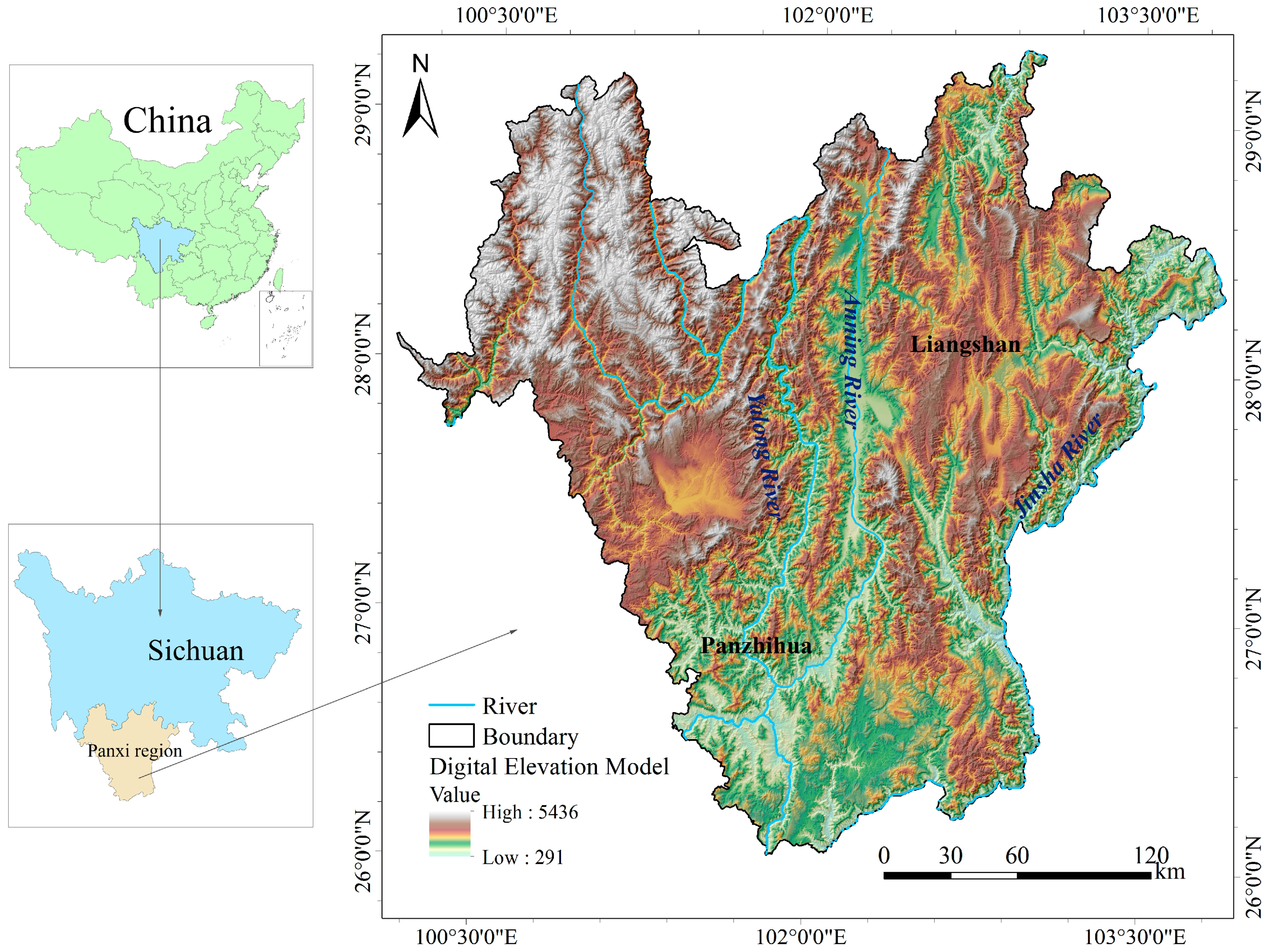
2. Overview of the Study Area

The Panxi region is located in southwest of Sichuan Province, China (Figure 1; 100°15′E to 103°53′E, 26°13′N to 29°27′N). Covering 67,500 km2 in area, it includes the city of Panzhihua and the Liangshan Yi Autonomous Prefecture. It borders the Tibetan Plateau to the north, the Yunnan-Guizhou Plateau to the south and the Sichuan Basin to the east. There are a variety of landforms, with mountains and hills predominating [41]. The terrain is higher in the northwest, and it is lower in the southeast; and deep river valleys are typical of the region, which has altitudes ranging between 291 and 5436 m. It has abundant water sources, including the Jinsha, Yanlong and Anning Rivers, among other branches of the Yangtze River. Meanwhile, with abundant mining resources, the Panxi region is one of China’s most important mining belts [42]. With the acceleration of urbanization and industrialization, demand for built-up land is rising, which has increased its encroachment on farmland. Moreover, economic development in the rural areas of Panxi is lagging behind the national average, and the production mode is extensive, so there are a series of inappropriate human activities occurring, such as deforestation and cultivation of marginal slope areas [43]. Consequently, the natural environment faces serious problems. In order to restore the natural environment, the Chinese Government conducted a pilot project in Sichuan Province in 1999 that investigated the return of farmland to forest and grassland. It advocated putting a halt to the development of land in slope areas that can potentially lead to soil erosion and to restore forests in suitable places so as to protect and enhance the regional environment.

3. Materials and Methods

3.1. Data Resources

The land use data used in this paper came from NASA’s Landsat Thematic Mapper(TM) remote sensing image data from 1990, 2000 and 2010, at a spatial resolution of 30 m. In the ENVI/ArcGIS platform, mosaic stitching, projection transformation and geometric correction, registration and other pre-treatments were conducted on the RS data. Land use types in Panxi region were divided into six categories (farmland, forest, grassland, water, built-up land and unused land) according to the land use/cover classification methods of the Resources and Environment Information Database of the Chinese Academy of Sciences (http://www.resdc.cn/). As the theme of this study is farmland change, farmland was divided into paddy field and dry land. Accuracy was evaluated by comparing the collected samples and the classified results. The comprehensive accuracy of all land use types is 90.02%, 86.7% and 73.82% in 1990, 2000 and 2010, which reaches the requirement of scientific research.
River and road data were derived from the National Earth System Science Data Sharing Infrastructure (http://www.geodata.cn/) [44], at a scale of 1:100,000. Using ASTER GDEM (V2), terrain data were taken from the National Engineering Research Center for Remote Sensing Applications and had a resolution of 30 m. Temperature and precipitation data were obtained from China Meteorological Administration (http://data.cma.cn). Based on terrain factors, we adopted the local thin plate spline method to conduct interpolation on temperature and precipitation and to obtain time series raster images of annual temperature and precipitation from 1990 to 2010, at a resolution of 1 km. The data of gross domestic production and population density were based on the yearbook of Sichuan province in 1991, 2001 and 2011.
According to the mountain classification standard based on actual conditions, the topology of Panxi is divided into 4 categories: the low altitude zone (altitude 0 to 2000 m; slope 0° to 8°), middle altitude zone (2001 to 3000 m; 15° to 25°), middle-high altitude zone (3001 to 4000 m; 15° to 25°) and high altitude zone (>4000 m; >25°). On the base of that, this study calculated the farmland change area of different altitudes and slopes and explored the driving forces of farmland change in different altitudes and slopes.

3.2. Study Methods

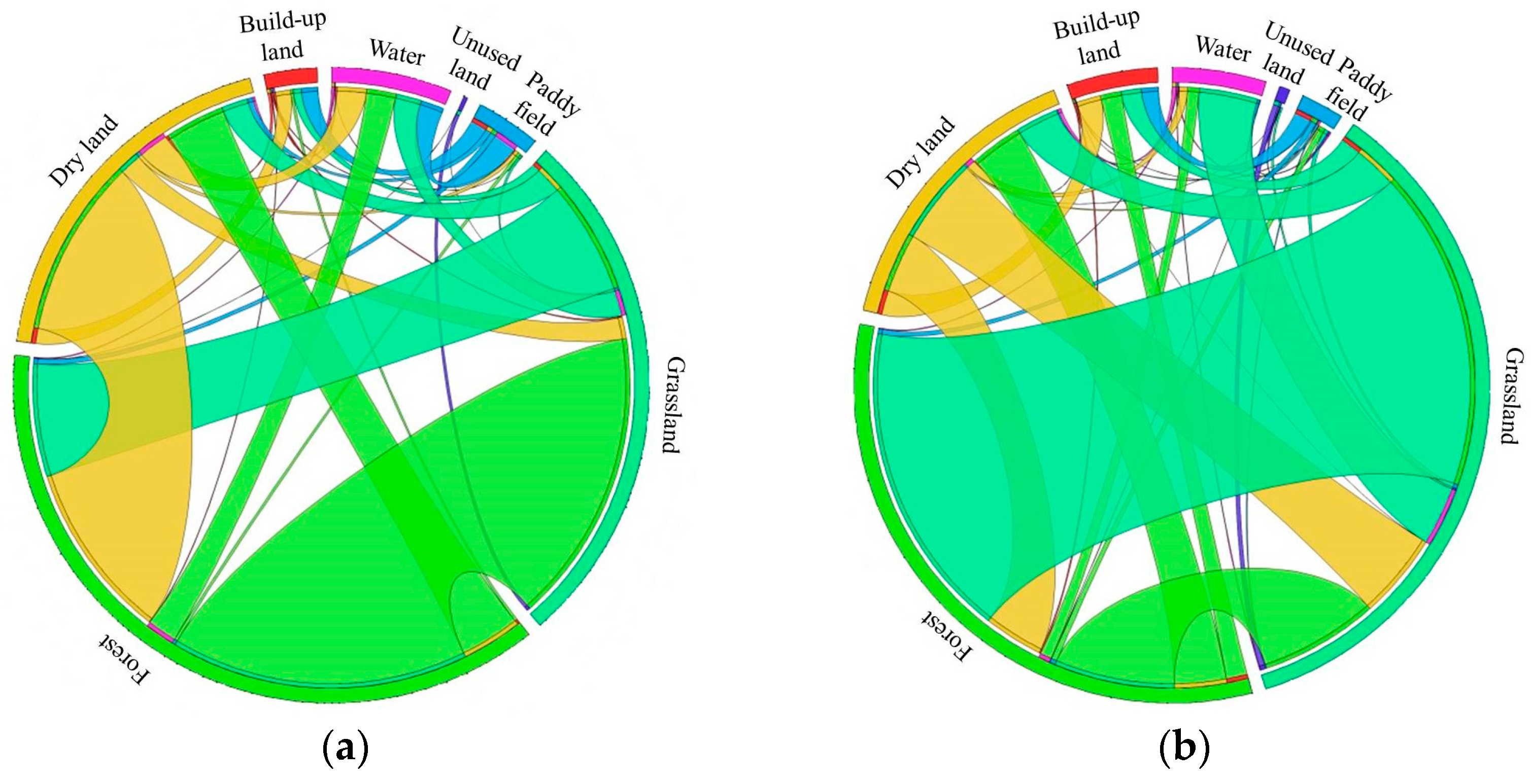
3.2.1. Land Use Transition Matrix

This matrix can comprehensively depict the detailed structure of regional land use dynamics, and reflect its direction. This method is derived from the quantitative description of system state and state transition in system analysis. It manifests the transformation process of one metastable system from T to T + 1 time and, thus, better reveals the spatiotemporal evolution of land use patterns. Its transition matrix is defined as follows [45]:
U   i j = [ U   11 U   12 ... U   1 n U   21 U   22 ... U   2 n ... ... ... ... U   n 1 U   n 2 ... U   n n ] ,
where i and j are the land use types, Uij is the land use state at the beginning and the end of the study time and n is the number of land use types.

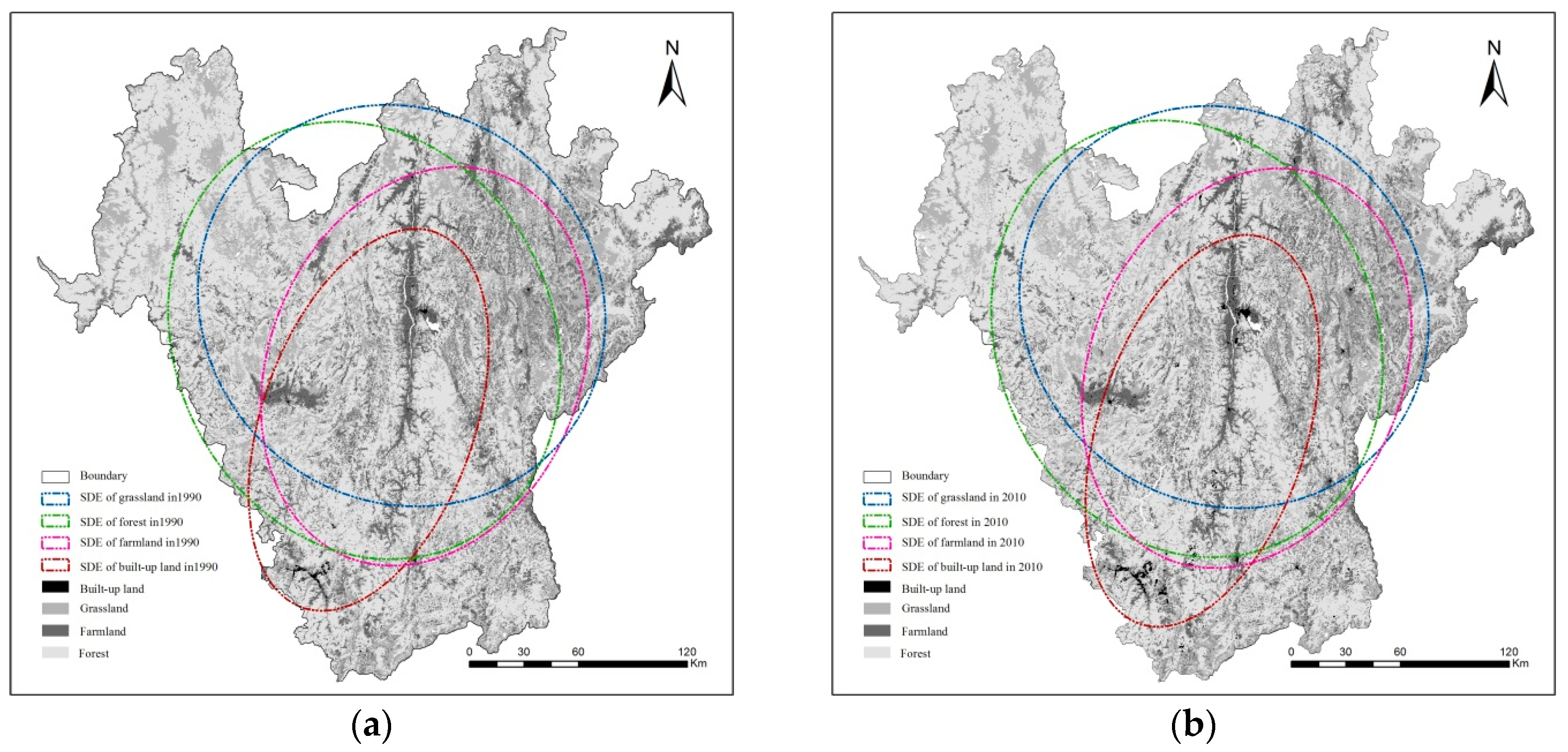
3.2.2. Standard Deviational Ellipse

Standard deviational ellipse is a common method used for measuring the trends of a set of points or regions according to the standard distance of directions x and y. Recently, It has been embedded in ArcGIS to analyze the distribution characteristics of point sets, and this method has been widely used [46]. The specific calculation process is given in [47].

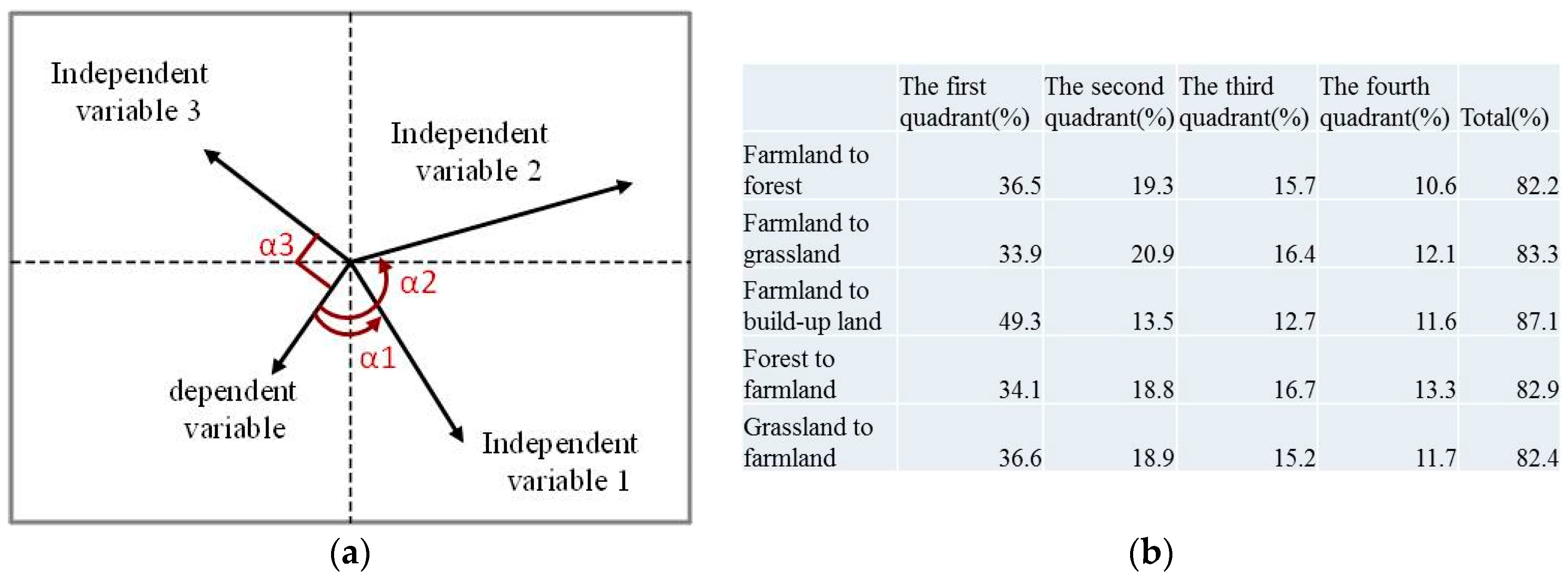
3.2.3. Principal Components Analysis

Principal components analysis (PCA) is a mathematical algorithm that reduces the dimensionality of data while retaining most of the variation in the dataset, which is the most widely used function. At the same time, PCA can also be used to study the correlation between the independent variable and the dependent variable, which is the purpose of this paper. Within the PCA sequencing diagram, if the angle between the independent variable and the dependent variable is smaller, their correlation is higher; on the contrary, their correlation is smaller. Additionally, their correlation size can be calculated through the formula of cosα. As shown in Figure 2a, the angle between the dependent variable and Independent Variable 1 is less than 90 degrees, namely cosα > 0, which means that their correlation is positive; the angle between the dependent variable and Independent Variable 2 is more than 90 degrees, namely cosα < 0, which means their correlation is negative; the angle between the dependent variable and Independent Variable 3 is 90 degrees, namely cosα = 0, which means they are not related. Before the correlation judgment, we should analyze the explanation degree of the independent variable to the dependent variable in each quadrant. Starting from the top right corner, each square is named as the first quadrant, the second quadrant, the third quadrant and the fourth quadrant in the counterclockwise direction. It is shown in Figure 2b that the explanation degree of the independent variable to the dependent variable is different in each quadrant, but their total explanation degree is over 80%. Therefore, we can conduct further analysis. All of these can be completed through CANOCO 4.5 software [48].

3.2.4. Driving Forces Selection

This study selected temperature, precipitation, elevation and slope [28] to represent natural factors, the distance to rivers and roads [29] to represent the effect of location and population density and gross domestic production [32] to show the human activities. Among them, the source and processing of temperature, precipitation, elevation and slope has been introduced in Section 3.1. The distance to rivers and roads was calculated through two steps. First, we calculated the distance of a grid to rivers (roads) in the study area. Second, we multiplied the weight of rivers (roads) with the distance to them and chose the minimum distance. In terms of population density and gross domestic production, we obtained the data of towns in the study area firstly, then rasterized the two indicators.

4. Results

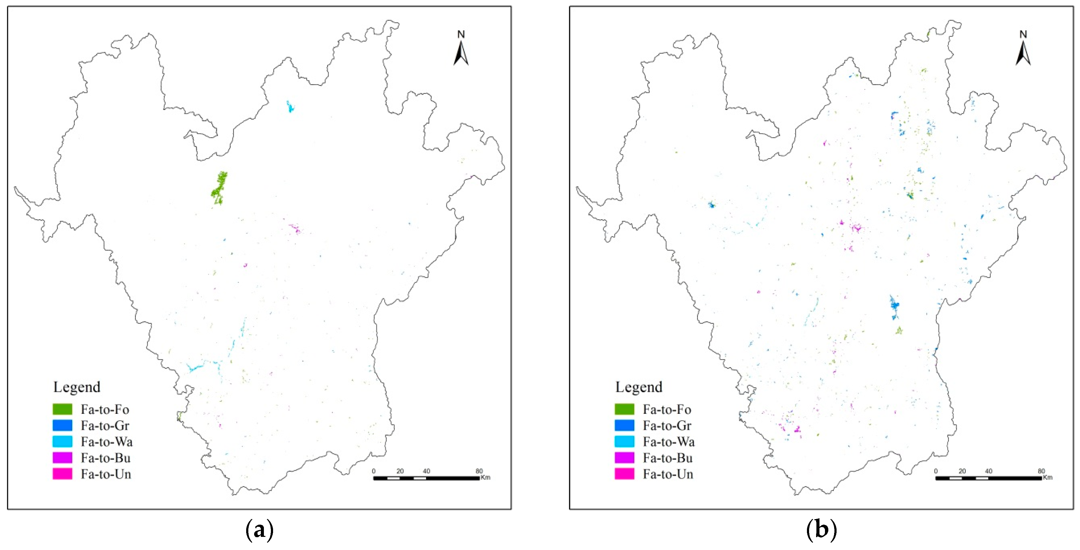
4.1. Farmland Changes in Panxi since 1990

Since 1990, farmland in Panxi region has decreased. It dropped from 11,834 km2 in 1990 to 11,521 km2 in 2010, falling at an average of 15.65 km2 per year (Table 1). From 1990 to 2010, dry land areas fell by 260 km2 and paddy fields reduced by 53 km2. The majority of farmland in Panxi is the dry land. Meanwhile, farmland area fell by 141 km2 during 1990 to 2000 and 172 km2 from 2000 to 2010. The decrease from 2000 to 2010 was higher than that of 1990 to 2000, which is probably because a policy of returning farmland to forest was implemented in 1999.
To analyze farmland dynamics in Panxi region since 1990, this study used a matrix table to reflect the farmland transfer course (Table 2). Transformation from farmland to other land types is called roll-out, while transformation from other land types to farmland is called roll-in. As indicated from the table, most roll-out was from farmland to forest, followed by grassland and built-up land, with roll-out areas of 257, 181and 101 km2, respectively. At the same time, large amounts of forest and grassland were turned into farmland. Their roll-in areas were 154.79 and 109.16 km2, respectively. As a whole, net transfer between farmland and forest covered the largest area, followed by built-up land and grassland. Their net transfer areas were 102.21, 92.84 and 71.84 km2, respectively. Hence, forest, built-up land and grassland are the major roll-out types of farmland. This also reflects that ecological construction projects have achieved certain effects. These included soil and water conservation projects and projects that returned farmland to forest upstream of the Yangtze River.
To analyze the spatial distribution of farmland and the three major land types, the standard deviational ellipse (SDE) of each land use type was drawn. Figure 3a,b shows that the standard deviational ellipse area for forest and grassland was obviously larger than that of farmland and built-up land, which means the distribution scope of forest land and grassland was broader. Among these, the standard deviational ellipse for farmland and built-up land has an egg shape, presenting a similar spatial distribution mode. To be specific, it shows an expanding tendency in a northeast-southwest direction and a shrinking state in the northwest-southeast direction. Its long axis is consistent with the direction of the Anning River, which means that water resources play a fundamental role for settlement and human production activities. In addition, the standard deviational ellipse for forest and grassland is round, with a larger spatial distribution. Its distribution is different from that of farmland and built-up land located in the northern part of Panxi region. The northern region has higher altitude and larger terrain differences. Hence, it can be seen that terrain has considerable influences on the distribution of forest and grassland. As a whole, farmland and built-up land, as well as forest and grassland share strong spatial interdependence and coherence.
As seen from angle θ (Table 3), the angle for farmland and built-up land was less than six degrees and for forest-grassland was less than 10 degrees. This also suggests that there was a closer relationship between farmland and built-up land, as well as between forest and grassland, in Panxi region. During 1990 to 2010, the y to x axis ratio in the standard deviational ellipses for farmland and grassland fell from 1.3236 and 0.9283 to 1.3235 and 0.9231, respectively. This means that the spatial distribution of farmland and grassland shrank, and the spatial dependency of each land type is increasing, as well. As for the y to x axis ratio in the standard deviational ellipses for built-up land and forest, they increased from 1.8741 and 0.8411 to 1.9424 and 0.8441 from 1990 to 2010, respectively. This suggests that the spatial distributions of built-up land and forest are expanding. Meanwhile, by comparing the y to x axis ratio in the standard deviational ellipses for various land types, a common trend of forest < grassland < farmland<built-up land exists at different time points, which indicates that the distribution of built-up land is most variable and influenced by human activities.

4.2. Farmland Transfer Characteristics of Different Stages in Panxi Region

This study investigated two periods of farmland changes. The chord diagram (Figure 4a) indicates that from 1990 to 2000, farmland was converted mostly from forest and grassland, which contributed 58.6% and 26.8% of the roll-in area of farmland, respectively. During the same period, some farmland was converted into forest land and water resources, with net transfer areas of 88.72 and 37.04 km2, respectively. This is because, in order to develop agriculture, Panxi region undertook many water conservancy projects. To improve water resource allocation capacity and save transportation costs, these projects were mainly built between farmlands and occupied some part of them. Moreover, Panxi region is a typically poor area, many rural youth chose to work outside in order to make much more money, which left the older people and children in the countryside. Because of the restriction of health, the older people could not engage in agricultural production activities, which need good physical strength. Therefore, a large amount of farmland became idle. Later, with the drive of protecting the environment, the government encouraged the older people to begin to plant trees in the idle land and gave them economic compensation, which promoted the transfer from farmland to forest. The chord diagram (Figure 4b) shows that from 2000 to 2010, some farmland was generated from forest and grassland, but farmland was mainly turned into grassland and built-up land, with net transfer areas of 76.22 and 74.74 km2, respectively. This is because Sichuan Province strived to develop a policy of Returning Farmland to Forest and Grassland and replace unsuitable farmland with grass and trees, which accelerated the transformation of farmland to grassland. Meanwhile, the urbanization of China increased in the new millennium. As a result, a rising urban population and industrialization have intensified the demand for built-up land. Hence, farmland around the cities became increasingly occupied, and built-up land areas increased significantly.
In this study, because the conversion area from other land use types to farmland is small and its spatial distribution is not obvious, we just consider the conversion area from farmland to other land use types; this can be summarized as follows: farmland to forest (Fa-to-Fo); farmland to grassland (Fa-to-Gr); farmland to water (Fa-to-Wa); farmland to built-up land (Fa-to-Bu); and farmland to unused land (Fa-to-Un). According to the distribution diagram for land transfer during 1990 to 2000 and 2000 to 2010 (Figure 5a,b), we can see that the spatial distribution of farmland transfer was much larger and broader during 2000 to 2010. From 1990 to 2000, regions that transformed from farmland to forest were mainly located on the west bank downstream of the Yalong River. Regions transforming from farmland to built-up land were located at Xichang City. Regions transforming from farmland to water were distributed in the Heishui River basin; and regions transforming from farmland to other types were relatively scattered. During 2000 to 2010, transformations from farmland to grassland shared a similar spatial distribution as conversions to forest land, which were mainly located at the Heishui River. Regions transforming from farmland to built-up land were mainly located in the Anning River valley and Panzhihua City; while transformation from farmland to other types was insignificant. Thus, it can be seen that the Heishui River basin and Anning River valley were the major regions with changes in farmland use. These two regions are also the essential regions for agriculture and settlements.

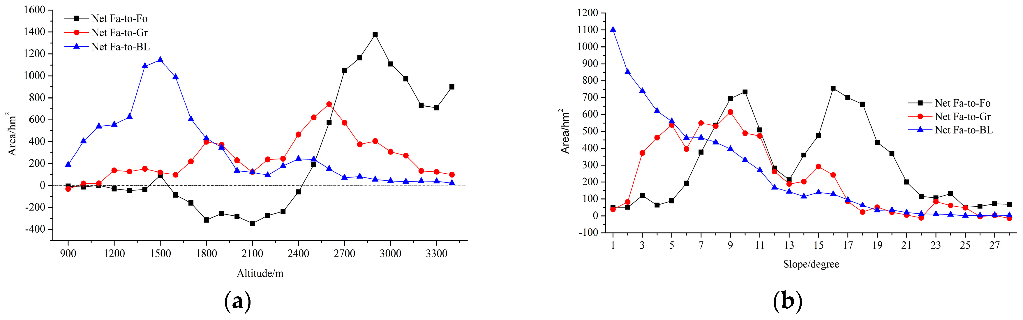
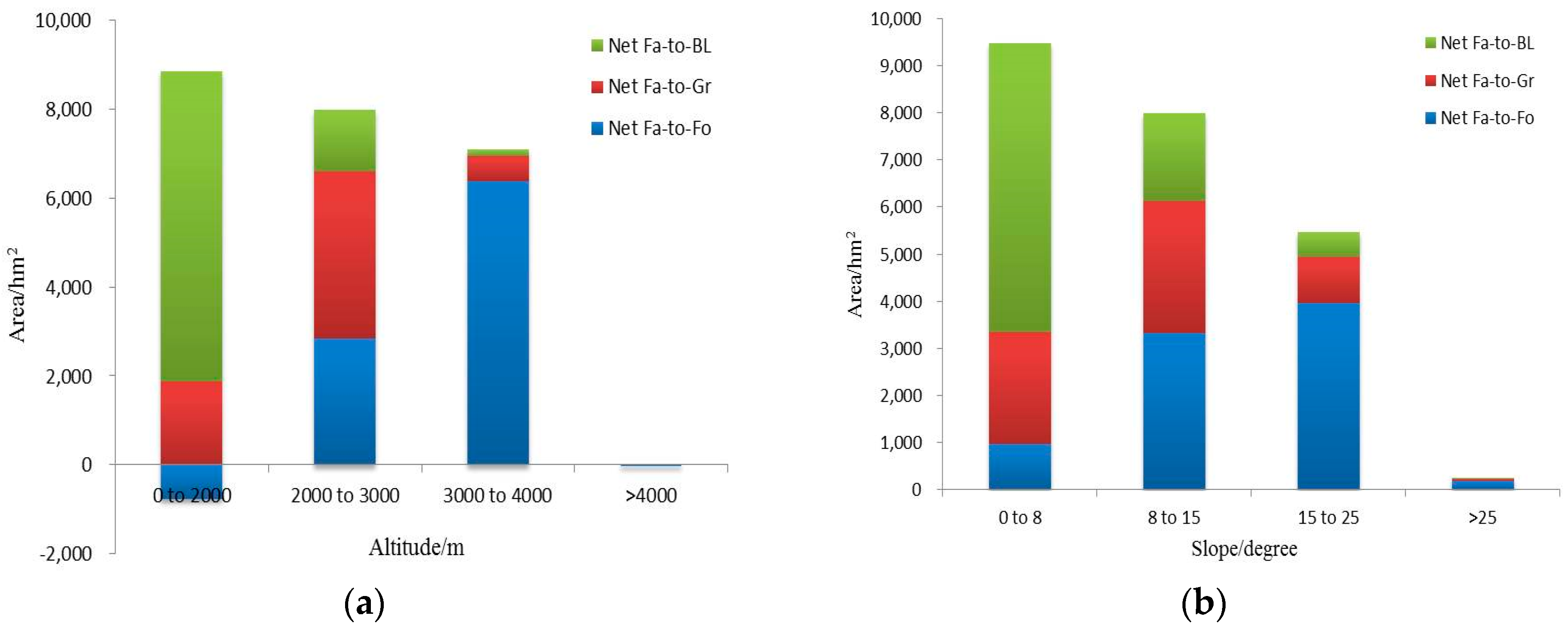
4.3. Farmland Dynamics across Different Terrains

As indicated in Figure 6a, there are significant differences in the net transformation characteristics of farmland to forest, grassland and built-up land. The net transfer area of farmland to built-up land (net Fa-to-BL) was larger than zero, showing a sharp rise and a fluctuating descending tendency. When altitude reached 1500 m, net Fa-to-BL reached its maximum. Net transformation area from farmland to grassland (net Fa-to-Gr) was also larger than zero, showing a fluctuating-rising and sharp-declining tendency. When the altitude reached 2600 m, net Fa-to-Gr reached its maximum value. Net transformation area of farmland to forest (net Fa-to-Fo) turned from negative to positive. When the altitude was <2500 m, net Fa-to-Fo was smaller than zero. This was manifested as forest transferring to farmland. When the altitude was >2500 m, net Fa-to-Fo was larger than zero, manifested as farmland being transferred to forest. Therefore, 2500 m can be regarded as the boundary point for the transformation between farmland and forest. As indicated from Figure 6b, net Fa-to-BL, net Fa-to-Gr and net Fa-to-Fo at different slopes were all larger than zero, indicating that farmland was transferred to other types of land. Among these, the transformation range from farmland to built-up land decreased at a faster pace in regions with less slope, and the fluctuations of net Fa-to-Gr and net Fa-to-Fo were larger. Meanwhile, when the slope was <7°, net Fa-to-BL was higher than that of grassland and forest. When the slope was >7°, net Fa-to-BL was lower than that of grassland and forest.
At the same time, with increasing altitude and slope, the net transformation area of farmland gradually declined (Figure 7a,b). Within this, net Fa-to-BL declined, while Fa-to-Fo increased, and Fa-to-Gr had a fluctuating tendency. At different altitudes or slopes, net farmland transformation direction varied. To be specific, low altitude or slope zones had the largest net Fa-to-BL. At middle altitude or slope zones, Fa-to-Gr was largest. Above middle altitude or slope zones, Fa-to-Fo was largest. Interestingly, at low altitude zones, net Fa-to-Fo was negative as forest was transferred to farmland due to agricultural development. Over time, due to the exploitation of forests and land reclamation, several ecological issues, such as land and soil erosion and desertification, arose. In order to ease these conflicts, Sichuan Province implemented a policy of Returning Farmland to Forest and Grassland in 1999. This included any farmland with slopes >15°. Net Fa-to-Fo has mainly occurred at slopes >15°, which demonstrates that the project of returning farmland to forest in Panxi has had considerable success.

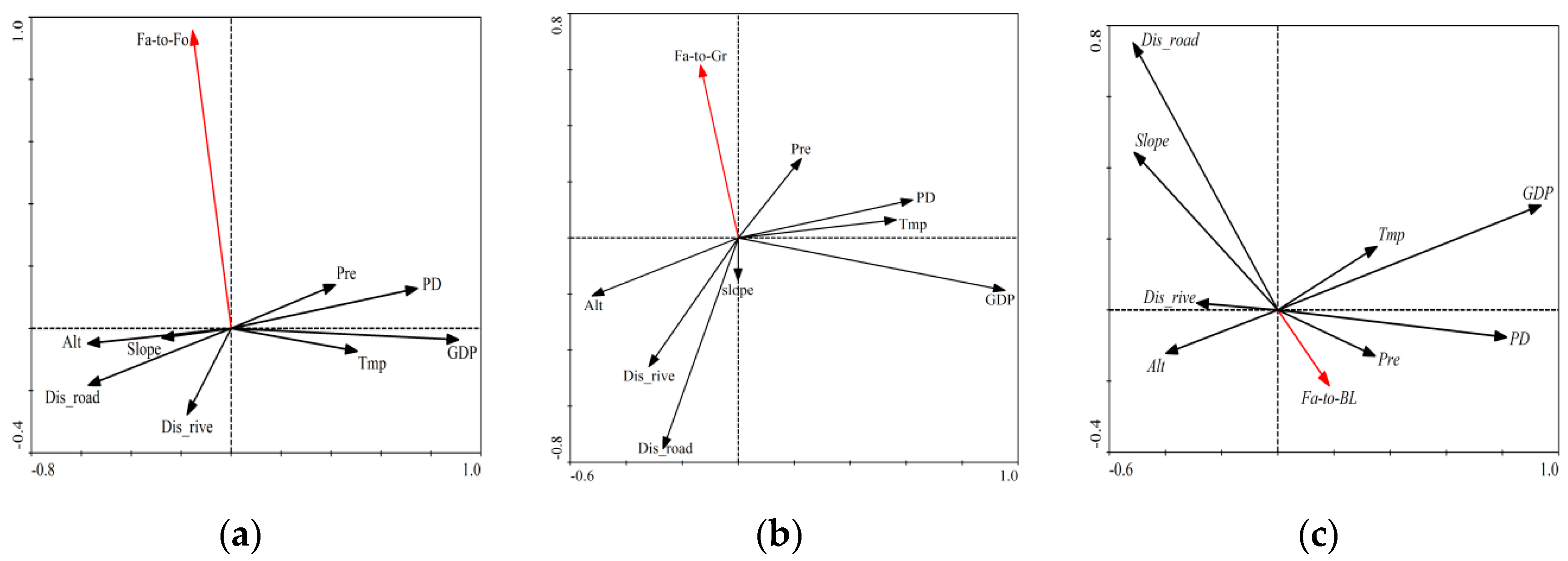
4.4. Driving Forces of Farmland Change

Due to restrictions on the availability of social and economic data, most existing studies of farmland dynamics in Panxi region have used the administrative unit as the sample with which to conduct econometric analyses, ignoring the heterogeneity within administrative units [49]. Some scholars have used a county or a small watershed as the research unit. Although this overcomes the limitations of using administrative units, their studies have been conducted at small scales, and there remains a lack of large-scale research [50]. Accordingly, considering the effectiveness and availability of the data, this study takes Panxi as an example, selects temperature (Tmp), precipitation (Pre), altitude (Alt), slope, the distance to rivers (Dis-river) and roads (Dis-road), population density (PD) and gross domestic product (GDP) to analyze their relationship with farmland changes in raster cells.

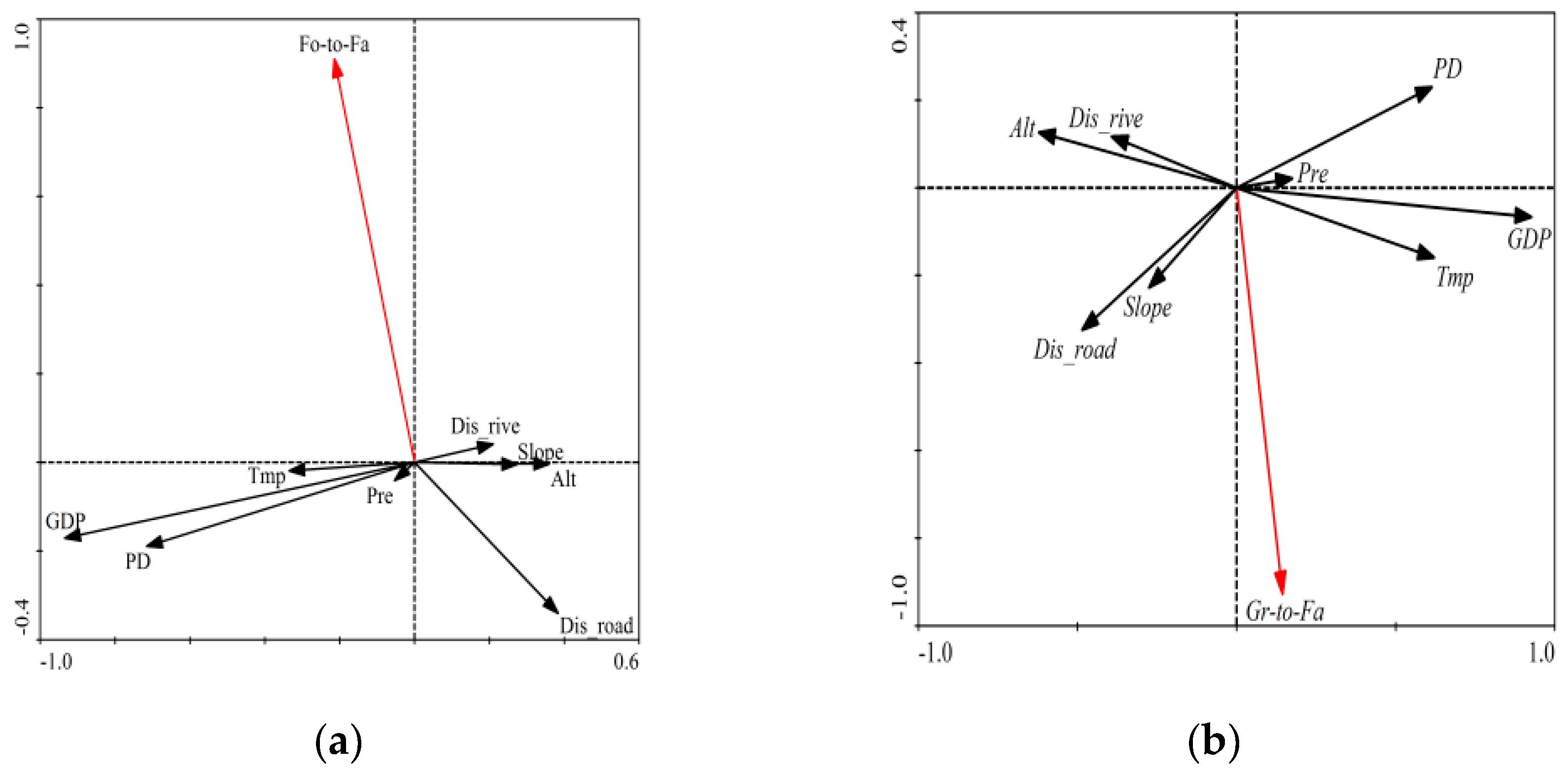
4.4.1. The Roll-out of Farmland

Figure 8 shows that the conversion of farmland to other land types was negatively related with Dis-river and Dis-road, and other factors were slightly different due to the land types to which farmland was transferred. In terms of Dis-river and Dis-road, the shorter the distance to a river or road, the better the accessibility of the area, and the increased ease with which human activities can be carried out. In particular, land use on both sides of roads has changed dramatically, characterized by increases in built-up land and agricultural land. This confirms that roads are key contributors to the conversion of farmland to built-up land. Meantime, in the pursuit of higher income, some young people in the countryside migrated to urban areas. This stimulated some farmers to convert crops to tree plantations, which require less labor input.

4.4.2. The Roll-in of Farmland

It can be seen from Figure 9 that the conversion of other land types to farmland was positively related with Tmp. The conversion of other land types to farmland was negatively related with PD and Alt, while other factors were significantly different due to the land types that were transferred to farmland. With rising temperatures, conditions become more favorable for crop growth, accelerating land exploitation and utilization. As the crucial agricultural production zone in Sichuan Province, the Ganre River valley increased its utilization of the land by making use of the advantageous light and heat conditions.
For regions with higher population densities, land is majorly applied to the construction of cities, in order to cater to population and industrial demands. That is to say, forest and grassland are mostly converted to built-up land and are rarely turned into farmland. By contrast, in regions with lower population densities that are far from the city and relatively poor, people mainly rely on agriculture for income. Hence, the transformation of forest and grassland is intended to provide areas suitable for farming. In 2006, the abolition of agricultural taxes and an increase in agricultural subsidies stimulated farmers to grow crops, while tree plantations become less profitable due to pest impacts. These factors motivated the conversion of forest and grassland to farmland.
In areas of high altitude, the climate causes a single land type, which is unsuitable for human habitation. Therefore, human disturbance is less frequent, and conversion to farmland is rare. Areas with low altitude have more people, so farmland around the town is easily converted to built-up land. However, to meet the demands of residents and the balance of demand and supply, most counties will develop new farmland away from the suburbs. Therefore, in low altitude areas, the probability of other land use types converted to farmland is greater than that of high altitude areas.

5. Discussion

Based on the land use data of Panxi region in 1990, 2000 and 2010, this study describes farmland dynamics and transfer characteristics through spatial econometric methods. We also discuss spatial heterogeneity due to altitude and slope and explore factors driving farmland change with principal component analysis.
Our results show that most of Panxi’s farmland was turned into forest and grassland from 1990 to 2010. The changes in Panxi were very different from those found in the plains of China, where farmland was mainly converted to built-up land. This was determined according to two aspects. The first was the orientation of Panxi region. A primary function of many counties in Panxi is to provide an ecological security barrier, which is the area for regional ecological protection, and the Chinese government has taken measures to protect the environment, while many counties have become the key objects of national ecological protection, which requires the restriction of large-scale urban development, such as Yanbian county. The second was the natural conditions in Panxi’s mountainous areas. To encourage development of the region, several economic measures were taken by the central government, but it was difficult to gather a large population, and many projects were unsuccessful because of geographical limitations. According to the statistics (Figure 10), Panxi’s urbanization has been increasing, but at a relatively slow rate of change. From 2000 to 2014, the urbanization rate in Panxi developed from 18.75% to 19.88%, only increasing1.13%. Its GDP in 2014 accounted for only 0.35% of the entire country, while its proportion of land area in the whole country is 0.7%, which demonstrated that the economic output per km2 of farmland was low.
This study presented some important issues about the relationship between land and water in Panxi. The standard deviational ellipse for forest and grassland showed a distinct landform-oriented tendency, which meant the forest and grassland were mainly distributed in the high-altitude area. This finding agrees with the fact that the net primary productivity (NPP) was higher in the same high-altitude area [51]. However, the standard deviational ellipse for farmland and built-up land followed the direction of the Anning River. This suggests that the presence of a river encourages land development. Therefore, settlements and infrastructure should be planned as close as possible to rivers in order to utilize land and water resources most efficiently. Meanwhile, the ratio of y to x axes in the standard deviational ellipse was the largest for built-up land, which meant the stability coefficient of built-up land was low, and there would be more freedom in selecting the location for built-up land when the abundance and security for water and land resources are relatively high [52].
Our study also identified two other interesting phenomena in Panxi. First, regional farmland has largely been turned into forest on slopes steeper than 15°. This inflection point differs from the standard one in China (≥25°), as identified in the Returning Farmland to Forest and Grassland policy. Due to the fragile ecological environment and the combination of intensified human activities, many areas with slopes less than 25° had already suffered from serious erosion. Hence, it is of practical significance for these farmland regions to return to forest land [53]. Second, at altitudes below 2500 m, there was a trend of forest conversion into farmland; at altitudes above 2500 m, the trend reversed. Thus, 2500 m tends to serve as a boundary between farmland and forest, which was close to the upper limit for population centers of Sichuan province (2600 m) [54]. Both of these findings indicate the presence of anthropogenic drivers for land use change.
To capture physical factors affecting farmland changes, this study focused first on temperature and precipitation. Then, in consideration of altitudinal differences, elevation and slope were included in the scope of influencing factors [55]. Finally, this study selected the distance to rivers (Dis-river) and roads (Dis-road) to represent the effect of location on farmland change. This decision was informed by previous studies that point out the relationship between a farm’s proximity to roads or rivers and that farm’s transformation possibility [56]. The indicators of physical factors are complete, and the results are reasonable. However, as for the anthropogenic factors, this paper only selected population density and GDP due to data restrictions. We did not consider the quantitative expression of agricultural production efficiency, labor migration or national policy in influencing farmland change, but such factors should be included in future research. It should also be noted that the method of principal component analysis used in this study to explore the driving forces is only based on present data and understanding. Further research is needed to monitor farmland change over longer periods of time to gain a better understanding of the relationships between human activities, natural factors and farmland change.
The spatial pattern of mountainous areas is broken, and the shape of most land use types is haphazard, which brings many challenges in land use interpretation. Therefore, our study adopted the Automated Registration and Orthorectification Package (AROP) to apply ortho-photo rectification and geometric registration to the images. Additionally, a classification scheme, which includes acquirement and expression of knowledge, as well as the application of knowledge in land use classification [57] and the fusion technology of multi-source remote sensing image [58], has been applied to obtain land classification. This approach was successful, and the classification accuracy is high (Table 4). When overlaying different spatial data for factor analysis, information was not lost, even though the resolution of the remote-sensing data was 30 m, and the topographic data were computed based on Shuttle Radar Topography Mission (SRTM) at a 90-mresolution with economic, population and climate data at a 1-km resolution. In conclusion, the results of this study are plausible.

6. Conclusions

In this study, we described farmland dynamics and transfer characteristics, discussed spatial heterogeneity due to altitude and slope, and explored driving factors of farmland change. Our findings were summarized as follows. The area of farmland change in Panxi region was 313 km2, only accounting for 2.6% of the region’s farmland. Farmland was mainly converted to forest and grassland as a result of the Returning Farmland to Forest Program. The expansion of water and built-up land was caused by urbanization and economic development. In terms of spatial distribution, the presence of water bodies influenced farmland and built-up land, while forest and grassland showed “landform-oriented” characteristics. The transfer between farmland and forest, grassland, built-up land dominated the farmland transition process. In terms of altitude, at altitudes <2500 m, the data displayed a trend of conversion from forest to farmland, while at >2500 m, this trend reversed. Thus, 2500 m serves as an altitudinal boundary between farmland and forest in Panxi. When comes to slope, The largest area of forest-farmland transfer occurred on slopes steeper than 15°, not 25°, as defined by China′s policy of Returning Farmland to Forest. As nature factors, the positive influence of temperature on farmland increasing and the negative impact of altitude on the increase of farmland was clear. For transportation, decreases in farmland were negatively correlated with proximity to rivers and roads. In the aspect of society, population density was negatively with the increasing of farmland.

Acknowledgments

This study was supported by the National Key Basic Research Program of China (973Program, 2015CB452706), the youth talent team program of the Institute of Mountain Hazards and Environment, Chinese Academy of Sciences (CAS) (SDSQB-2015-01), the National Natural Science Foundation of China (41401198 and 41571527) and the Youth Innovation Promotion Association, CAS (No. 2016332).

Author Contributions

Li Peng, Tiantian Chen and Shaoquan Liu. Li Peng and Shaoquan Liu conceived and designed the research; Tiantian Chen and Li Peng conducted the literature review; Tiantian Chen and Li Peng analyzed the data; Tiantian Chen and Li Peng wrote the paper. Li Peng and Tiantian Chen contributed equally to this work.

Conflicts of Interest

The authors declare no conflict of interest.

References

  1. Yu, B.; Lu, C. Change of cultivated land and its implications on food security in China. Chin. Geogr. Sci. 2006, 16, 299–305. [Google Scholar] [CrossRef]
  2. Long, H.L.; Zou, J. Grain production driven by variations in farmland use in China: An analysis of security patterns. J. Resour. Ecol. 2010, 1, 60–67. [Google Scholar]
  3. Reidsma, P.; Tekelenburg, T.; Van den Berg, M.; Alkemade, R. Impacts of land use change on biodiversity: An assessment of agricultural biodiversity in the European Union. Agric. Ecosyst. Environ. 2006, 114, 86–102. [Google Scholar] [CrossRef]
  4. Qin, Y.W.; Liu, J.Y.; Shi, W.J.; Tao, F.L.; Yan, H.M. Spatial-temporal changes of cropland and climate potential productivity in northern China during 1990–2010. Food Secur. 2013, 5, 499–512. [Google Scholar] [CrossRef]
  5. Wang, Y.; Scott, S. Illegal farmland conversion in China’s urban periphery: Local regime and national transitions. Urban Geogr. 2009, 29, 327–347. [Google Scholar] [CrossRef]
  6. Thorson, J.A. Zoning Policy Change and the Urban Fringe Land Market. Real Estate Econ. 1994, 22, 527–538. [Google Scholar] [CrossRef]
  7. Abelairas-Etxebarria, P.; Astorkiza, I. Farmland prices and land use changes in periurban protected natural areas. Land Use Policy 2012, 29, 674–683. [Google Scholar] [CrossRef]
  8. Brady, M.; Kellermann, K.; Sahrbacher, C.; Jelinek, L. Impacts of decoupled agricultural support on farm structure, biodiversity and landscape mosaic: Some EU results. J. Agric. Econ. 2009, 60, 563–585. [Google Scholar] [CrossRef]
  9. Stoate, C.; Baldi, A.; Beja, P.; Boatman, N.D.; Herzon, I.; van Doorn, A.; De Snoo, G.R.; Rakosy, L.; Ramwell, C. Ecological impacts of early 21st century agricultural change in Europe to a review. J. Environ. Manag. 2009, 91, 22–46. [Google Scholar] [CrossRef] [PubMed]
  10. Stoate, C.; Boatman, N.D.; Borralho, R.J.; Carvalho, C.R.; De Snoo, G.R.; Eden, P. Ecological impacts of arable intensification in Europe. J. Environ. Manag. 2001, 63, 337–365. [Google Scholar] [CrossRef]
  11. Ackrill, R.; Kay, A.; Morgan, W. The common agricultural policy and its reform: The problem of reconciling budget and trade concerns. Can. J. Agric. Econ. 2008, 56, 393–411. [Google Scholar] [CrossRef]
  12. Wang, G.; Liu, Y.; Li, Y.; Chen, Y. Dynamic trends and driving forces of land use intensification of cultivated land in China. J. Geogr. Sci. 2015, 25, 45–57. [Google Scholar] [CrossRef]
  13. Zhu, H.Y.; Li, X.B.; Xin, L.J. Intensity change in cultivated land use in China and its policy implications. J. Nat. Resour. 2007, 22, 907–915. [Google Scholar]
  14. HAASE, D. Effects of urbanization on the water balance—A long-term trajectory. Environ. Impact Assess. Rev. 2009, 29, 211–219. [Google Scholar] [CrossRef]
  15. York, R. Demographic trends and energy consumption in European Union Nations 1960–2025. Soc. Sci. Res. 2007, 36, 855–872. [Google Scholar] [CrossRef]
  16. Poyatos, R.; Latron, J.; Llorens, P. Land use and land cover change after agricultural abandonment: The case of a Mediterranean mountain area (Catalan Pre-Pyrenees). Mt. Res. Dev. 2003, 23, 362–368. [Google Scholar] [CrossRef]
  17. Deng, W.; Fang, Y.P.; Tang, W. The strategic effect and general directions of urbanization in mountain areas of China. Bull. Chin. Acad. Sci. 2013, 28, 66–73. [Google Scholar]
  18. Ministry of Agriculture of the People’s Republic of China. Available online: http://www.moa.gov.cn/govpublic/ZZYGLS/201412/t20141217_4297895.htm (accessed on 15 June 2016).
  19. Li, J.; He, C.; Shi, P. Change process of cultivated land and its driving forces in Northern China during 1983–2001. Acta Geogr. Sin. 2004, 59, 274–282. [Google Scholar]
  20. Verburg, P.H.; Veldkamp, A.; Fresco, L.O. Simulation of changes in the spatial pattern of land use in China. Appl. Geogr. 1999, 19, 211–233. [Google Scholar] [CrossRef]
  21. Veldkamp, A.; Lambin, E.F. Predicting land use change. Agric. Ecosyst. Environ. 2001, 85, 1–6. [Google Scholar] [CrossRef]
  22. Veldkamp, A.; Verburg, P.H. Modelling land use change and environmental impact. J. Environ. Manag. 2004, 72, 1–3. [Google Scholar] [CrossRef] [PubMed]
  23. Zhang, X.Z.; He, F.N.; Li, S.C. Reconstructed cropland in the mid-eleventh century in the traditional agricultural area of China: Implications of comparisons among datasets. Reg. Environ. Chang. 2013, 13, 969–977. [Google Scholar] [CrossRef]
  24. Baja, S.; Arif, S. GIS-Based Modelling of Land Use Dynamics Using Cellular Automata and Markov Chain. J. Environ. Earth Sci. 2014, 4, 61–66. [Google Scholar]
  25. Nagendra, H.; Munroe, D.K.; Southworth, J. From pattern to process: Landscape fragmentation and the analysis of land use/land cover change. Agric. Ecosyst. Environ. 2004, 101, 111–115. [Google Scholar] [CrossRef]
  26. Pijanowski, B.C.; Brown, D.G.; Shellito, B.A. Using neural networks and GIS to forecast land use changes: A land transformation model. Comput. Environ. Urban Syst. 2002, 26, 553–575. [Google Scholar] [CrossRef]
  27. Waiyasusri, K.; Yumuang, S.; Chotpantarat, S. Monitoring and predicting land use changes in the Huai Thap Salao Watershed area, Uthaithani Province, Thailand, using the CLUE-s model. Environ. Earth Sci. 2016, 75, 1–16. [Google Scholar] [CrossRef]
  28. Ostwald, M.; Chen, D. Land use change: Impacts of climate variations and policies among small-scale farmers in the Loess Plateau, China. Land Use Policy 2006, 23, 361–371. [Google Scholar] [CrossRef]
  29. García-Frapolli, E.; Ayala-Orozco, B.; Bonilla-Moheno, M. Biodiversity conservation, traditional agriculture and ecotourism: Land cover/land use change projections for a natural protected area in the northeastern Yucatan Peninsula, Mexico. Landsc. Urban Plan. 2007, 83, 137–153. [Google Scholar] [CrossRef]
  30. Fernández-Romero, M.L.; Lozano-García, B.; Parras-Alcántara, L. Topography and land use change effects on the soil organic carbon stock of forest soils in Mediterranean natural areas. Agric. Ecosyst. Environ. 2014, 195, 1–9. [Google Scholar] [CrossRef]
  31. Dang, Y. The agricultural development of Hexi Corridor and its influence on ecological environment in historic times. Collect. Essays Cniness Hist. Geogr. 2001, 16, 114–126. [Google Scholar]
  32. Mottet, A.; Ladet, S.; Coqué, N. Agricultural land use change and its drivers in mountain landscapes: A case study in the Pyrenees. Agric. Ecosyst. Environ. 2006, 114, 296–310. [Google Scholar] [CrossRef]
  33. Venteris, E.R.; Slater, B.K. A comparison between contour elevation data sources for DEM creation and soil carbon prediction, Coshocton, Ohio. Trans. GIS 2005, 9, 179–198. [Google Scholar] [CrossRef]
  34. Li, Y.; Shao, J.; Zhou, G. Genesis Difference of Rocky Desertification in Karst Mountains-A Case Study of Panxian County, Guizhou Province. Sci. Geogr. Sin. 2007, 27, 785–790. [Google Scholar]
  35. Friedmann, H. The political economy of food: A global crisis. New Left Rev. 1993, 197, 29–57. [Google Scholar]
  36. McMichael, P. A food regime genealogy. J. Peasant. Stud. 2009, 36, 139–169. [Google Scholar] [CrossRef]
  37. Long, H.L.; Heilig, G.K.; Li, X.B.; Zhang, M. Socio-economic development and land use change: Analysis of rural housing land transition in the Transect of the Yangtse River, China. Land Use Policy 2007, 24, 141–153. [Google Scholar] [CrossRef]
  38. Jobbagy, E.G.; Jackson, R.B. The vertical distribution of soil organic carbon and its relation to climate and vegetation. Ecol. Appl. 2000, 10, 423–436. [Google Scholar] [CrossRef]
  39. Lu, Y.; Xu, Y.; Cai, Y. Analysis on Land Use/Land Cover Changes of Small Drain Basin Based on RS and GIS. Sin. Prog. Geogr. 2005, 1, 9. [Google Scholar] [CrossRef]
  40. Schneeberger, N.; Bürgi, M.; Hersperger, A.M. Driving forces and rates of landscape change as a promising combination for landscape change research—An application on the northern fringe of the Swiss Alps. Land Use Policy 2007, 24, 349–361. [Google Scholar] [CrossRef]
  41. Su, C.J.; Xu, Y.; Fang, Y.P. Bio-resource exploitation and ecological and environmental construction-Taking Panxi area as an example. J. Mt. Sci. 2004, 22, 143–148. [Google Scholar]
  42. Wang, X.G. Patterns and tactics for agro-economic development in ecotone—A case study from Panxi region in Sichuan province. Ecol. Agric. Res. 1994, 2, 24–30. [Google Scholar]
  43. Wang, F.L.; Zhan, T.P.; Chen, W. Advances in study of Nb-Ta ore deposits in Panxi area and tentative discussion on genesis of these ore deposits. Miner. Depos. 2012, 31, 293–308. [Google Scholar]
  44. The National Earth System Science Data Sharing Infrastructure. Available online: http://www.geodata.cn/ (accessed on 23 July 2016).
  45. Qiao, W.F.; Sheng, Y.H.; Fang, B.; Wang, Y.H. Land use change information mining in highly urbanized area based on transfer matrix: A case study of Suzhou, Jiangsu Province. Res. Geogr. 2013, 32, 1497–1507. [Google Scholar]
  46. Lefever, D.W. Measuring geographic concentration by means of the standard deviational ellipse. Am. J. Sociol. 1926, 32, 88–94. [Google Scholar] [CrossRef]
  47. Wang, L.C.; Gao, J. The Spatial Coupling Relationship between Settlements and Land-Water Resources in Zhangye Irrigation Districts. Ecol. Geogr. 2014, 2, 21. [Google Scholar] [CrossRef]
  48. Šmilauer, P.; Lepš, J. Multivariate Analysis of Ecological Data Using CANOCO 5; Cambridge University Press: Cambridge, UK, 2014. [Google Scholar]
  49. Liao, C.M.; Liu, Y.H.; Hu, B.Q.; Yan, Z.Q.; Zhou, X. Atlas analyses of karst l and rocky desertification and ecological rehabilitation model. Trans. Chin. Soc. Agric. Eng. 2004, 20, 266–271. [Google Scholar]
  50. Lu, Y.G.; Xu, Y.Q.; Cai, Y.L. Analysis on land us/land cover changes of small drain basin based on RS and GIS. Sin. Prog. Geogr. 2005, 24, 79–86. [Google Scholar]
  51. Wang, Q.; Zhang, T.B.; Yi, G.H.; Chen, T.T.; Bie, X.J.; He, Y.X. Tempo-spatial variations and driving factors analysis of net primary productivity in the Hengduan mountain area from 2004–2014. Acta Geogr. Sin. 2017, 37. [Google Scholar] [CrossRef]
  52. Sun, P.L.; Xu, Y.Q.; Wang, S. Terrain gradient effect analysis of land use change in proverty area around Beijing and Tianjin. Trans. Chin. Soc. Agric. Eng. 2014, 30, 277–288. [Google Scholar] [CrossRef]
  53. Luo, H.B.; Qian, X.G.; Liu, F.; He, T.B.; Song, G.Y. Ecological Benefit of Soil and Water Conservation in Hilly Areas by De farming and Reafforestation. J. Soil Water Conserv. 2003, 17, 31–34. [Google Scholar]
  54. Guo, J.M. Analysis on Population Distribution and Influencing Factors in Sichuan; Sichuan Normal University: Chengdu, China, 2014. [Google Scholar]
  55. Liu, M.; Hu, Y.M.; Chang, Y. Landscape change and its spatial driving force of farmlands in Wenchuan County of Minjiang River upper reach. Chin. J. Appl. Ecol. 2007, 18, 569–574. [Google Scholar]
  56. Chen, Z.; Lu, C.; Fan, L. Farmland changes and the driving forces in Yucheng, North China Plain. J. Geogr. Sci. 2012, 22, 563–573. [Google Scholar] [CrossRef]
  57. Yang, C.J.; Zhou, C.H. Investigation on classification of remote sensing image on basis of knowledge. Geogr. Territ. Res. 2007, 17, 72–77. [Google Scholar]
  58. Sun, J.B.; Liu, J.L.; Li, J. Multi-source remote sensing image data fusion. J. Remote Sens. 1998, 2, 47–50. [Google Scholar]
Figure 1. Location of Panxi region, China.
Sustainability 08 01209 g001
Figure 2. (a) The correlation judgment between the dependent variable and the independent variable; (b) explanation degree of the independent variable to the dependent variable in each quadrant.
Sustainability 08 01209 g002
Figure 3. Standard deviational ellipses of four land use types in (a) 1990 and (b) 2010.
Sustainability 08 01209 g003
Figure 4. Chord diagram of farmland, Panxi region: (a) 1990 to 2000; (b) 2000 to 2010.
Sustainability 08 01209 g004
Figure 5. Spatial distribution of farmland converted to other land use types, Panxi region: (a) 1990 to 2000; (b) 2000 to 2010. Farmland to forest (Fa-to-Fo); farmland to grassland (Fa-to-Gr); farmland to water (Fa-to-Wa); farmland to built-up land (Fa-to-Bu); and farmland to unused land (Fa-to-Un).
Sustainability 08 01209 g005
Figure 6. The relationship of net conversion area between farmland and the other three land types at different (a) altitudes and (b) slopes.
Sustainability 08 01209 g006
Figure 7. Comparison of net farmland conversion at different (a) altitudes and (b) slopes.
Sustainability 08 01209 g007
Figure 8. Driving forces of the conversion from farmland to forest (a); grassland (b); and built-up land (c). Alt, altitude; PD, population density; Dis, distance; Pre, precipitation; Tmp, temperature.
Sustainability 08 01209 g008
Figure 9. Driving forces of the conversion from forest (a) and grassland (b) to farmland.
Sustainability 08 01209 g009
Figure 10. Change of urbanization rate in Panxi region since 2000.
Sustainability 08 01209 g010
Table 1. Change of farmland in Panxi region since 1990.
Area199020002010Reduced Area 1990 to 2000Reduced Area 2000 to 2010
Paddy field/km22126209620733023
Dry land/km2970895979448111149
Total/km211,83411,69311,521141172
Table 2. Transition matrix table of farmland in Panxi region, 1990 to 2010 (km2).
2010Paddy FieldDry LandForestGrasslandWaterBuilt-up LandUnused Land
1990
Paddy Field06.40115.4571.719.60940.7420
Dry Land4.9350235.868170.09836.10255.6530.099
Forest12.355136.811573.644414.92843.43141.5490.582
Grassland8.8891.107663.75717.188129.59643.4193.17
Water0.9455.8282.0211.82710.340.6870
Built-up Land1.0842.4840.2970.5241.7272.090
Unused Land3.12400.13311.8251.45700
Table 3. Parameters of standard deviational ellipses of four land types in Panxi region. SDE, standard deviational ellipse.
YearLand TypesAngleSDE-xSDE-yRatio of y and x
1990Farmland22.685,786.2113,546.61.3236
Forest154.5124,007.6104,297.80.8411
Grassland129115,589.8107,304.10.9283
Built-up land19.558,534.6109,700.11.8741
2010Farmland22.9886,080.6113,927.61.3235
Forest155.1123,551.9104,295.30.8441
Grassland128.45116,193.2107,254.70.9231
Built-up land17.6657,551.7111,7861.9424
Table 4. Accuracy verification of different land use types in 1990, 2000 and 2010.
Year199020002010
Land Use Type
Farmland93.10%86.50%65.04%
Forest86.90%83.75%75.94%
Grassland89.60%84%74%
Water92.50%88%72.73%
Built-up land89%91%85.19%
Unused land89%87%70%
Comprehensive accuracy90.02%86.70%73.82%

