Article

Spatiotemporal Variation of China’s State-Owned Construction Land Supply from 2003 to 2014

1
Key Laboratory of Land Surface Pattern and Simulation, Institute of Geographic Sciences and Natural Resources Research, Chinese Academy of Sciences, Beijing 100101, China
2
University of Chinese Academy of Sciences, Beijing 100049, China
*
Author to whom correspondence should be addressed.
Sustainability 2016, 8(11), 1137; https://doi.org/10.3390/su8111137
Submission received: 22 September 2016 / Revised: 28 October 2016 / Accepted: 2 November 2016 / Published: 4 November 2016
(This article belongs to the Special Issue Governing the Transformation of Urban Infrastructures)

Abstract

:
State-owned construction land is the dominant legal land source for construction in China and its supply influences urban expansion, house prices, and economic development, among other factors. Surprisingly, limited attention has been directly devoted to the spatiotemporal variation in land supply or the driving factors. This paper applied a centroid model and hotspot analysis, and created a newly increased construction land dependence-degree index (NCD) to present the spatiotemporal variations of China’s construction land supply magnitude and pattern from 2003 to 2014, using land supply data from 339 cities. A two-way fixed effect model was introduced to reveal the influence of the socio-economic driving factors. The results showed that China’s state-owned construction land supply area (CLSA) and newly increased construction land supply area (NCSA) both increased during the period from 2003 to 2014, the geographic centroid of CLSA and NCSA moved northwest. NCD showed an overall increasing trend, and hotspots with high NCD migrated from the east region to the west region and shifted from an “east hot and west cold” pattern in 2003 to an “east cold and west hot” pattern in 2014. The gross domestic product (GDP) has a U-shape effect on CLSA and NCD. The population, average annual wage of workers, and investment in fixed assets (fiv) have positive effects on CLSA, and fiv also has a positive effect on NCD. The increasing ratio of tertiary industry added value to secondary industry added value reduces CLSA and NCD, and the effects of state policies vary from year to year. Different land supply policies should be implemented for cities in different development stages.

1. Introduction

Urban expansion is common in the process of urbanization around the world [1]. Rapid urban expansion is observed in many countries, particularly in developing countries, such as India [2] and Malaysia [3]. Land is the physical base of urban expansion, and urban expansion requires a lot of land for construction. It has resulted in enormous problems, such as farmland loss [4], fragmentation [5], and urban sprawl [6]. Reasonable land supply is crucial to reduce these problems.
As the largest developing country, China is undergoing a similar process of rapid urbanization, and has tremendous demands for construction land [7]. From 2003 to 2014, China’s urbanization rate increased from 40.5% to 54.8%, with an average annual growth of 1.3%; further, its construction land increased from 31.1 million ha to 38.1 million ha, with an average annual growth of 640 thousand ha [8]. Meanwhile, China’s arable land area decreased dramatically [9,10]. According to the China Land and Resources Statistical Yearbook, an average of approximately 230 thousand ha of arable land was converted into built-up land annually over this period. Because China has a vast population and scarce land per capita, the conflict between urban expansion and arable land loss is bound to affect both food security and sustainable economic development [10,11].
All land in China is public and the land market is strongly controlled by the state, which is quite different from other countries. In China’s land use right system, the land is divided into the state-owned and collective-owned land in the term of land ownership [12]. Generally, urban land is owned by the state, and rural land is owned by rural collective economic organizations. Urban development has to be conducted on the state-owned land, and rural land cannot be used for urban development. The conversion of rural land to urban purposes is controlled by the government through land expropriation (some compensation must be provided, and ownership of agricultural land is also converted from collective-owned to state-owned). Only state-owned land can be sold on the land market to individuals or corporations, whereas collective-owned land must go through government land expropriation to be supplied as construction land [13,14]. As a consequence, stated-owned construction land is the dominant legal supply source for construction. Therefore, as the largest land source of urban city expansion in China, the stable supply of state-owned construction land can alleviate the conflict mentioned above because much of this land is converted from arable land. Conversely, irrational supply, including oversupply, results in negative impacts, such as urban sprawl, the production of “ghost cities”, and the over-conversion of farmland [15,16,17].
In 2003, China’s land policy changed dramatically, and land supply policy, along with fiscal and monetary policies, was applied as a major part of national macro-control measures to deal with the overheated economy and constrain rural-urban land over-conversion [18]. In recent years, the Chinese government has frequently used this tool to control house prices in response to escalating house prices [19,20,21]. Moreover, Chinese government announced that the supply-side structural reform would be enacted in response to the economic “new normal” in late 2015 [22,23]. Land is the carrier of economic activity, thus the adjustment in the structure and magnitude of land supply is an important part of the reform, which can force the industry to update and promote the reform process.
As mentioned above, land supply is a key factor that affects urban expansion, house prices, and economic development. Thus, there are a growing number of studies that examine land supply and its relationship to urban expansion, economic development, house prices, and government policies. Some scholars argue that land supply is a crucial factor influencing housing price fluctuation and impacts the risk of a housing bubble [21,24,25,26], and different land supply channels also have an impact on the housing supply and price [27]. Population growth and increasing income both affect construction land supply from the perspective of urban expansion, which is the result of construction land supply [28,29,30,31,32]. The relationship between economic development and land supply is not simply linear [33,34]. Government policies, such as a restricted land use policy, land financing, and government intervention, influence the demand for land and thus affect land supply [35,36,37].
Surprisingly, limited attention has been directly devoted to spatiotemporal variation and driving factors of land supply. Understanding the variation and driving factors is crucial to improving the reasonability of construction land supply and land use intensity. Rational construction land supply can meet reasonable urban construction land demands, prevent urban sprawl, and reduce the pressure of farmland loss, and then promote sustainable area development.
The main aims of this study were: (1) to reveal the spatiotemporal variation in the magnitude and pattern of China’s state-owned construction land supply and (2) to quantitatively analyze the influences of socio-economic driving factors on land supply. The results can enhance our understanding of land supply and help policy-makers formulate rational land supply plans and policies to make reasonable and efficient use of construction land, which can provide new insights into reasonable and sustainable area development.

2. Materials and Methods

2.1. Materials

As mentioned above, China’s land policies centered on land supply became national macro-control measures in 2003. Meanwhile, for-profit construction land, including industrial land, was stipulated to be supplied by municipal governments through “tender, auction, or listing”, which resulted in the land supply in China becoming market-oriented [38]. Thus, we selected 2003 as the beginning of this study.
Data for the state-owned construction land supply area (CLSA) and newly increased construction land supply area (NCSA) (2003–2014) at the municipal level were derived from the China Land and Resources Statistical Yearbook (2004–2015) [39] issued by the Ministry of Land and Resources of China. State-owned construction land supply area in this study refers to granting land supply area.
Municipal socio-economic data for the period (2002–2014) were obtained from the China City Statistical Yearbook (2003–2015) [40] issued by the National Bureau of Statistics of China. The data included gross domestic product (GDP), population (pop), investment in fixed assets (fiv), and average annual wage of workers (wage). Additionally, the secondary industry as a percentage of GDP and tertiary industry as a percentage of GDP were used to calculate the ratio of tertiary industry added value to secondary industry added value (ratio).
Due to the administrative division adjustment and missing data, the data from the yearbooks were reconsolidated to ensure the continuity and consistency of the data. The China Land and Resources Statistical Yearbook (2004–2015) contains the land supply data of 352 administrative Units totally. Twelve of them are special administrative units, such as municipality directly under the provincial government and county-level city, and their land supply data are not continuous. The socioeconomic data of three cities (i.e., Haidong city, China; Bijie city, China; and Tongren city, China) in the 290 cities contained in the China City Statistical Yearbook (2003–2015) are also discontinuous. Therefore, they were excluded from our study. Moreover, Chaohu city in Anhui province China was downgraded to county-level city in 2011, and was administered by Hefei city. So we merged the land supply and socioeconomic data of Chaohu city into the data of Hefei city, China. Finally, consistent land supply data from 339 cities were generated to study the temporal and spatial variations. Socio-economic data from 286 cities were obtained to study the socio-economic driving factors of land supply quantitatively. Due to data limitations, Hong Kong, Macao, and Taiwan were not included in this study.

2.2. Methods

2.2.1. Construction Land Supply Centroid Model

A centroid model is a critical tool that is used to analyze spatiotemporal variations of features that occur during the process of regional development. It can image the movement of the centers of gravity through the coordinate system to accurately express the regional differences and highlight the spatial expression of regional differences. The method has been widely used in the fields of economics [41], ecosystem services [42], energy production and consumption [43], crop production centroids [44], and land use change [45] etc. We used the centroid model to calculate the geographical centroids of CLSA and NCSA to reveal their spatiotemporal variation dynamically. The model examines the dynamics of the centroid throughout the study period and estimates the locations (longitudeand latitude) of the centroids of CLSA and NCSA, respectively. Based on the calculation formulas of center of gravity applied in land use science [46], the coordinates of a centroid were calculated using Equation (1).
l o n t = i = 1 n A i , t × l o n t / i = 1 n A i , t ;    l a t t = i = 1 n A i , t × l a t t / i = 1 n A i , t
where lont and latt are the longitude and latitude of the geographical centroids of CLSA or NCSA in year t, respectively; loni and lati are the longitude and latitude of the geographical centroid of city i, respectively; Ai,t is the CLSA for year t in city i when calculating the centroids of CLSA, and the NCSA when calculating the centroids of NCSA; and n is the total number of all cities.
The calculation and mapping of CLSA and NCSA centroids was conducted using ArcGIS 10.0 (Esri, Redlands, CA, USA) (http://www.esri.com/software/arcgis/arcgis-for-desktop).

2.2.2. Newly Increased Construction Land Dependence-Degree Index (NCD)

The state-owned construction land supply can be divided into newly increased construction land supply and existing construction land supply. The newly increased construction land dependence-degree index (NCD), which is the ratio of NCSA to CLSA, reflects the dependence of city development on newly increased construction land supply. A high NCD indicates that urban expansion is the dominant land use, whereas a low NCD means the city’s land use is more focused on inner potentials. The NCD of each city was calculated using Equation (2).
N C D i , t = ( N C S A i , t / C L S A i , t ) × 100 %
where NCDi,t is the NCD of city i in year t; NCSAi,t is the NCSA of city i in year t; and CLSAi,t is CLSA of city i in year t.

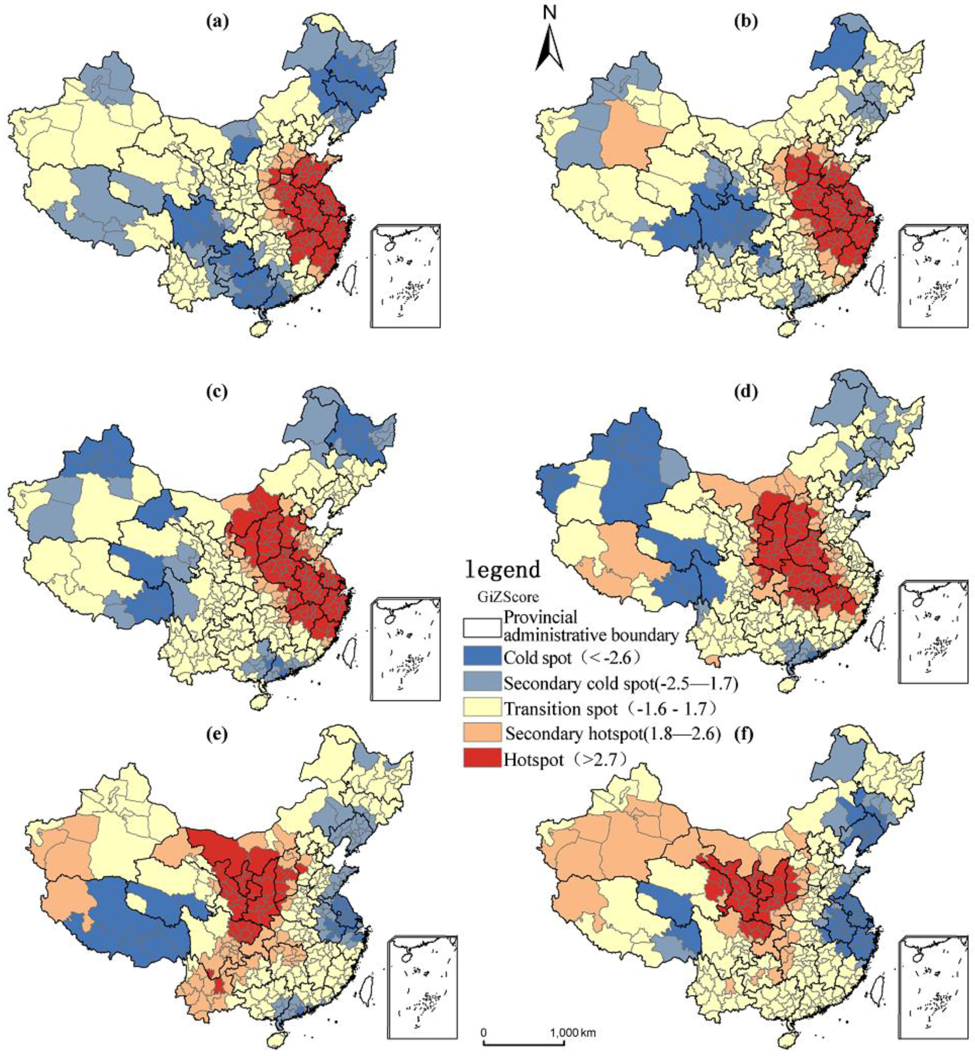
2.2.3. Hotspots Analysis

To reveal the variation in the NCD pattern, we used hotspots analysis, which calculated the Getis-Ord Gi* statistic for the NCD of each city [47]. The resultant Gi* statistic is a z-score that indicates where high or low NCD values are spatially clustered. If the Gi* is positive and statistically significant, the city is identified as a hot spot, which implies it is surrounded by other cities with high NCD values. If the Gi* is negative and statistically significant, the city is identified as a cold spot, which implies it is surrounded by other cities with low NCD values. The Getis-Ord Gi* statistic was calculated using Equation (3) in ArcGIS 10.0.
G i , t * = ( j = 1 n w i j , t N C D j , t N C D t ¯ j = 1 n w i j , t ) / ( S [ n j = 1 n w i j , t 2 ( j = 1 n w i j , t ) 2 ] / ( n 1 ) )
where G i , t * is the Gi* value of city i in year t; N C D ¯ t = j = 1 n N C D j , t / n ; S = j = 1 n N C D j , t 2 / n ( N C D t ¯ ) 2 ; n is the number of cities; wij,t is the one/zore spatial weight between city i and j in year t. If city i and j are adjacent, wij,t will have a value of 1, otherwise 0; NCDj,t is the NCD of the city j in the year t; and N C D ¯ t is the mean of NCD values from all cities in year t.

2.2.4. Two-Way Fixed Effect Model

Regression analyses have been widely used to analyze complex issues [48,49,50]. Two panel data regression models were used to quantitatively analyze the socio-economic factors that drive CLSA and NCD. As mentioned above, these factors include economic development, population growth, living level, state policy, local government intervention. We selected GDP, ratio, and fiv to represent economic development levels and patterns; pop to represent population growth; wage to represent living level; and year dummies (yrt) to represent state policy and local government intervention. As linearity is necessary in the model and the heteroscedasticity should be avoided or reduced as much as possible, we transformed the values of CLSA, pop, GDP, fiv, and wage into natural logarithms. Moreover, after the log transformation, an elasticity model was obtained to describe the elasticity of construction land supply area to the socio-economic factors.
Furthermore, we performed the Hausman test to select the appropriate model, and the results indicated that the fixed-effect model was better than the random-effect model. To simultaneously account for individual fixed effects and time period fixed effects, we constructed two-way fixed effect models. The regression models were described as Equations (4) and (5), examining the drive factors of CLSA and NCD, respectively.
ln C L S A i , t =   c + β 1 ln G D P i , t + β 2 ( ln G D P i , t ) 2 + β 3 ln p o p i , t + β 4 ln w a g e i , t + β 5 ln f i v i , t + β 6 r a t i o i , t + yr t + ε i , t
N C D i , t =   c + β 1 ln G D P i , t + β 2 ( ln G D P i , t ) 2 + β 3 ln p o p i , t + β 4 ln w a g e i , t + β 5 ln f i v i , t + β 6 r a t i o i , t + yr t + ε i , t
where CLSAi,t is the CLSA of city i in year t; NCDi,t is the NCD of city i in year t; βs (s = 1, …, 6) are the regression coefficients of the influencing factors; εi,t is the random error term; and yrt is the time period fixed effects with no individual differences but varying with time and represents the dummy variable of each year from 2004 to 2014, respectively. The year 2003 was used as a base and excluded to avoid perfect collinearity; c is the constant.
To avoid endogenous problems, the one-year lagging values of GDP and fiv were used. All price-related variables, including GDP, fiv, and wage, were deflated to real values as of 2003 using the consumer price index (CPI) published in the China Statistical Yearbook. We ran the models with the STATA 12.0 (StateCorp, College Station, TX, USA) (http:// www.stata.com/).

3. Results and Discussions

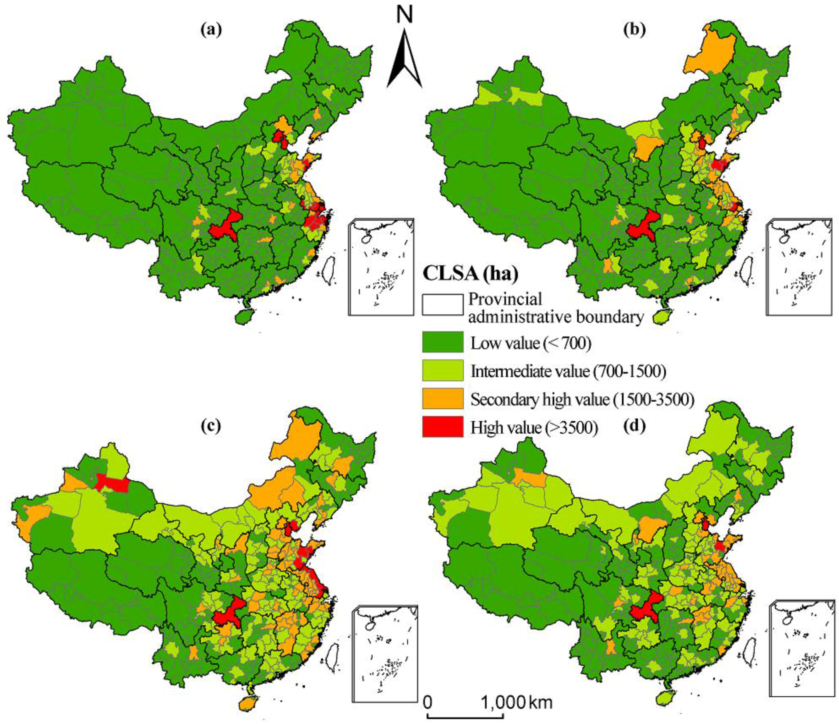
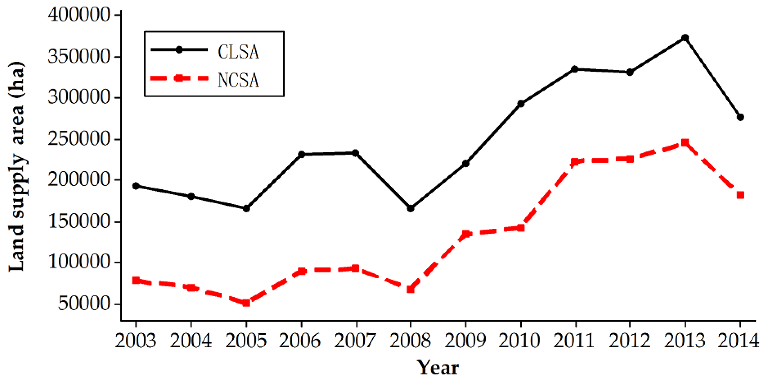
3.1. Spatiotemporal Variation of CLSA

CLSA increased from 192.9 thousand ha to 276.8 thousand ha, a difference of approximately 7000 ha annually, over the period from 2003 to 2014 (Figure 1). The increasing trend can be divided into three stages: downward fluctuation from 2003 to 2008; a rapid increase from 2008–2011; and slow growth followed by downward fluctuation from 2011 to 2014.
Figure 2 showed the values of municipal CLSA for 2003, 2009, 2013, and 2014. The municipal CLSA values in 2003 were generally low. In 2003, there were 272 cities with low values, accounting for 80.24% of the total area, and they were mainly distributed in central and western China. There were 36 cities with intermediate values, accounting for 10.62% of the total area, and they were mainly distributed in the eastern Huang-Huai Plain. There were 31 cities with high and secondary values, accounting for 9.14% of the total area, and they were distributed in the Yangtze River Delta, the Beijing-Tianjin region, and Chongqing.
In 2009, the intermediate and secondary high value areas spread westward to Jiangxi Province, western Hebei Province, and eastern Inner Mongolia. In 2013, the intermediate and secondary high value areas continued to spread westward, and these areas appeared in eastern and central China. There were 11 cities with high values, accounting for 3.24% of the total area, and they were distributed in the coastal cities of Jiangsu Province, the hilly region of Shandong Province, and Chongqing. There were 66 cities with secondary values, accounting for 19.74% of the total area, and these cities were mainly distributed in the eastern Inner Mongolia, the north portion of North China Plain, and the Yangtze Plain. The number of cities with intermediate values increased to 124, accounting for 36.58% of the total area, and these cities were mainly distributed in the western Inner Mongolia, the northern Gansu Province, the western Huang-Huai Plain, and the Zhejiang-Fujian hilly region. The number of cities with low values drastically decreased to 138, accounting for 40.71% of the total area, and these cities were mainly distributed in Tibet, the Yunnan-Guizhou Plateau, and the western Sichuan Province, China.
Compared to 2013, the CLSA decreased dramatically in 2014 and the distribution also changed considerably. The numbers of cities with high and secondary values was reduced to 3 and 38, respectively, and they were mainly distributed in Jiangsu Province, the central Anhui Province and the hilly region of Shandong Province. The number of cities with intermediate values also reduced to 111, and these areas were mainly distributed in Xinjiang, Inner Mongolia, and central China. The number of cities with low values increased to 184, and they were mainly distributed in western China.
In general, cities with high and intermediate values gradually spread from eastern China to western China, which is the main characteristic of CLSA spatiotemporal variation from 2003 to 2014.

3.2. Spatiotemporal Variation of NCSA

The variations in the trend of NCSA from 2003 to 2014 were similar to that of CLSA (Figure 1). The NCSA increased from 76.6 thousand ha in 2003 to 181.7 thousand ha in 2014, a rate of approximately 8.7 thousand ha annually. The trend could also be divided into three stages: downward fluctuation from 2003 to 2008; a rapid increase from 2008 to 2011; and slow growth followed by downward fluctuation from 2011 to 2014.
Figure 3 showed the values of municipal NCSA in 2003, 2009, 2013, and 2014. The municipal NCSA values in 2003 were also generally low. In 2003, there were 291 cities with low values, accounting for 85.84% of total area. These areas were mainly distributed in the central and western regions of China. There were 17 cities with intermediate values, accounting for 5.07% of the total area. The distribution was scattered in the North China plain and Chongqing. There were a total of 31 cities with high and secondary high values, accounting for 9.14% of the total area. These areas were distributed in the Yangtze River Delta, the coastal cities of Jiangsu Province, and Beijing.
In 2009, the cities with middle and high values spread westward to Jiangxi Province, the western Hebei Province, the eastern and central Inner Mongolia and the central Anhui Province. In 2013, cities with middle and high value had become widespread across China. There were 75 cities with high values, accounting for 22.12% of the total area, and they were distributed in Yangtze River Delta, the North China Plain, the Sanjiang Plain, Jiangxi Province, central Guizhou Province, and northern Gansu Province. There were 80 cities with secondary high values, accounting for 23.16% of the total area, and they were mainly distributed in the central Inner Mongolia, Shanxi Province, Henan Province, and the northern Fujian Province. The number of cities with intermediate values increased to 105, accounting for 30.97% of the total area, and they were mainly distributed in Inner Mongolia, Hunan Province, and Yunnan Province. The number of cities with low values reduced dramatically to 79, accounting for 23.3% of the total area. Areas with low values were mainly distributed in Tibet, southern Qinghai Province, and western Sichuan Province.
Consistent with CLSA, NCSA decreased dramatically in 2014 and the distribution changed considerably. The number of cities with high and secondary high values reduced to 111 in total. The cities that shifted from the high and secondary high values to intermediate and low values were concentrated in the central and eastern regions, which may be the result of China’s economic downturn in 2014 and the slowing of GDP growth leading to the suppressed demand for NCSA. It is worth noting that NCSA in the cities of the Yunnan-Guizhou Plateau and Tibet remained low from 2003 to 2014.
In general, the cities with high and secondary high values gradually spread from China’s eastern regions to western regions at a higher rate than total CLSA, which is the main characteristic of NCSA spatiotemporal variation from 2003 to 2014.

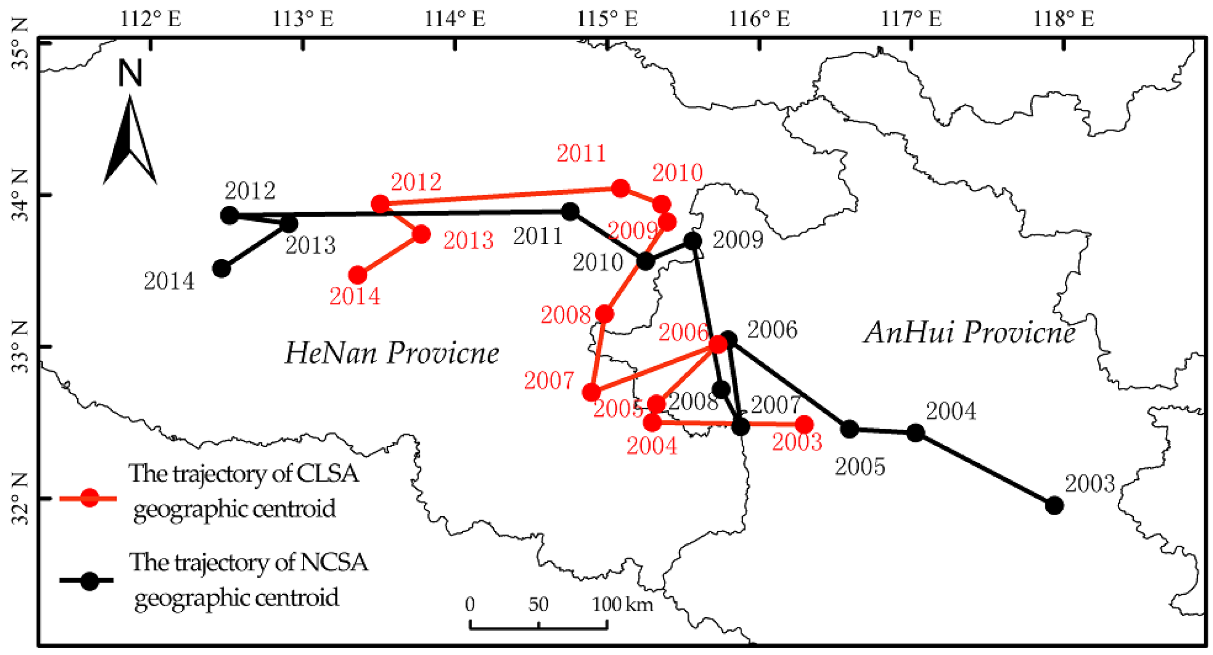
3.3. Position and Movement of CLSA and NCSA Geographic Centroids

We used the aforementioned centroid model to calculate the geographic centroids of the CLSA and NCSA in each year from 2003 to 2014 (Table 1), then mapped the trajectories of their movement (Figure 4).
The centroid of CLSA moved northwest at an average of 5.9 km annually from the northwestern Anhui Province to the central Henan Province. The geographic centroid of NCSA also had a northwest trajectory and moved at an average of 7.5 km annually, further than the geographic centroid of CLSA, from the southeast Anhui Province to the west Henan Province.
Specifically, CLSA geographic centroid moved mainly northwest at an average speed of 5.8 km/year from 2003 to 2010 and turned southwest at an average speed of 6.1 km/year beginning in 2010. The gravity center of NCSA moved from the southeast to the northwest at an average speed of 7.7 km/year from 2003 to 2009 and turned west at an average speed of 7.3 km/year beginning in 2009.

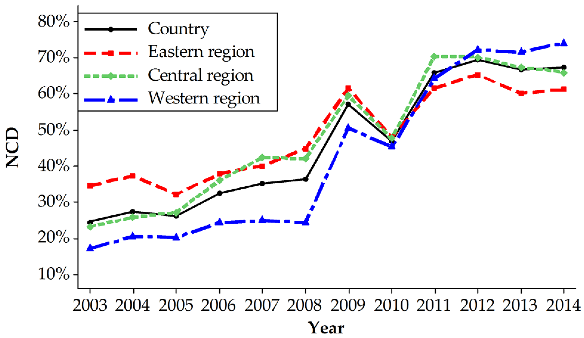
3.4. Spatiotemporal Variation of NCD

At the national scale, NCD increased from 24% of the total area in 2003 to 67% of the total area in 2014, more than doubling the area over this period (Figure 5). NCD increased steadily from 2003 to 2008. NCD fluctuated during the period from 2008 to 2011, with significant yearly increases and decreases, although the overall increase was larger than the decrease. Since 2011, NCD remained steady at approximately 67% and changed slightly.
The variations in the NCD in the eastern, central, and western regions of China from 2003 to 2010, were almost consistent. In all three regions, there was an upward trend, and the central region’s NCD growth was slightly higher than those of the other two regions. The eastern region had the highest NCD, the central region was in the middle, and the western region had the lowest. The gap between the three regions narrowed from 2003 to 2010. From 2010 to 2012, the central and western regions’ NCDs grew more rapidly than did that of the eastern region. The central region had the highest NCD, the western region was in the middle, and the western region had the lowest. After 2012, the NCD of the three regions remained steady, with the western region increasing slightly, and the central and eastern regions decreasing slightly. The order of the three regions’ NCD was western region as the highest, the central region in the middle, and the eastern region lowest after 2012, which was the opposite of the order from 2003 to 2010. This order shift showed that in the eastern region, the degree of dependence of development on newly increased construction land decreased, land use intensity increased, and land use type shifted from urban expansion to utilizing internal potentialities via urban redevelopment [51,52]. The lower dependence was also the result of strict limitation policies set on the land supply in the major cities [38,53].
Figure 6 showed the results of NCD hotspot analysis. In 2003, hotspots were concentrated in the northeastern coastal cities and the central region, whereas cold spots were mainly located in Guangxi Province, Guangdong Province, Guizhou Province, Sichuan Province, and the northeast area.
In 2006, hotspots spread to the northwest area; the southern Shanxi Province became a new hotspot, northern Shaanxi Province became a secondary hotspot. The area of cold spots decreased, with cold spots mainly located in Sichuan Province, Tibet, and the southeastern Qinghai Province.
In 2009, hotspots continued to spread to the northwest. The Loess Plateau in the northern Shaanxi Province and the Ordos Plateau in central Inner Mongolia became new hotspots, forming a centralized hot belt from the Yangtze River Delta to the Loess Plateau. Cold spots continued to shrink and were mainly concentrated in the northeastern region, northern Qinghai Province and southeastern Tibet.
The hotspots in 2011 displayed an overall moving trend, mainly located in the northern Jiangxi Province, Hubei Province, Henan Province, Shanxi Province, Shaanxi Province, Ningxia, and central Inner Mongolia. The Yangtze River Delta was no longer a hotspot in 2011. The cold spots in 2011 were mainly distributed in Xinjiang, Qinghai, and the northeastern region.
In 2013, the hotspot areas continually moved west. The concentration of hotspots occurred around the Loess Plateau and the Sichuan Basin. The Yunnan-Guizhou Plateau and the Hubei-Hunan Plateau became secondary hotspots. Due to expanding limitation policies in large cities, as well as industry updating and transfer, the Yangtze River Plain and the hilly region of Shandong Province became the concentration areas of cold and secondary cold spots, respectively.
In comparison with 2013, the hotspots in 2014 declined to some extent. The hotspots were mainly distributed in Shaanxi, Ningxia, Gansu, and Sichuan. The secondary hotspots moved from the Yunnan-Guizhou Plateau to the Xinjiang district. The number of cold spots in the western region decreased, and the cold spots in the eastern coastal region expanded, forming an “east cold and west hot” pattern. This shift was possible because of the implementation of the “Belt and Road Initiative” along with the undertaking of industrial transfer policies by the western regions. In addition, cities in the western region were mostly in the initial development stage and depended heavily on the newly increased construction land, which might be another reason.

3.5. Analysis of Socio-Economic Driving Factors

We conducted a Likelihood-ratio (LR) test, a Wooldridge (2002) test, and a Pesaran (2004) test, which showed that the heteroscedasticity, first-order autocorrelation, and cross-sectional correlation all existed. Thus, Driscoll and Kraay’s covariance estimator was implemented to modify the model, which provided more robust results. Due to space limitations, we only report the more robust regression results modified by Driscoll and Kraay measure. The estimation results of the two-way FE model are presented in Table 2.
GDP has a noticeable impact on both CLSA and NCD. In both models, the coefficients of lnGDP are significantly positive, and the coefficients of (lnGDP)2 are significant negative. The coefficients of lnGDP and (lnGDP)2 indicate that GDP has a U-shaped effect on both CLSA and NCD, which means that CLSA and NCD first increase and then decrease with the growth of GDP. This is possible because at the initial stage of the economic development, a multitude of demands for infrastructure and its supporting facilities combined with rough use of land lead to increased demand for construction land. Then, with further economic development, the expansion of construction land will be decoupled from economic growth, with more and more developed construction land being used, and land-use trends are becoming more intensive, resulting in a decrease of CLSA and NCD [54]. The results also can explain, to some extent, the aforementioned spatiotemporal variations of CLSA and NCD.
Population (pop) has a significant effect on CLSA, but an insignificant effect on NCD. The coefficient of pop to CLSA is 0.168 and is significant at the 10% level. This indicates that each 1% increase in pop increases CLSA by 0.168% when other factors are controlled. Population growth results in increasing demands for house, transportation, urban green space, and other related facilities, therefore, raising CLSA. The coefficient measured in our study is consistent with the findings of previous studies [31]. However, the coefficient of pop to NCD is negative and insignificant, which means the population is not the main driving force for NCD. To improve land use intensity and alleviate the conflict between urban development and farmland loss, China’s central government encourages local government to use existing construction land, and imposes more stringent regulatory constraints on new construction land supply. The substitution of newly increased construction land of existing construction land may lead to the consideration that the population is not the main driving force for NCD [18,33]. In addition, driven by an incentive to maximize benefits of land leasing and the pressure from developers to acquire land, local governments were trapped by an oversupply of land [55,56]. Therefore, newly increased construction land supply was driven by the ambition of local governments to raise local revenue and attract investment through land granting, instead of population growth. The oversupply of construction land, an irrational land supply, demonstrates that population is not the main driving force for NCD. It is an irrational aspect of land supply in China. The oversupply leads to high real estate inventory in most of China’s small and medium-sized cities. The local government should supply construction land more according to population growth rather than land revenue to avoid oversupply of land, which is conducive to sustainable urban development.
The average annual wage of workers (wage) is one of the main driving factors of CLSA, but does not have a significant impact on NCD. The coefficient of wage to CLSA is 0.165 and is significant at the 10% level, which indicates that each 1% increase in wage increase CLSA by 0.165% when other factors are controlled. The increase in the wage of workers will promote the improvement of their living conditions, thereby increasing the demand for construction land and promoting the supply of construction land. The coefficient of wage to NCD is only −0.002, which is low and insignificant. This indicates that wage has a little effect on NCD, and is not the main driving factor of NCD.
Investment in fixed assets (fiv) has a significantly positive effect on both CLSA and NCD. The elasticity of fiv to CLSA is 0.199 and is significant at the 1% level. This means that each 10% increase in fiv increases CLSA by 1.99%. These results indicate that investment in fixed assets can promote the supply of construction land, which is consistent with previous studies [28,30]. The elasticity of fiv to NCD is 0.022 and is significant at the 1% level, which means that investment in fixed assets can also promote NCD to some extent.
The ratio of tertiary industry added value to second industry added value (ratio) has a significantly negative effect on both CLSA and NCD. When other factors are controlled, each 1% increase in ratio could trigger a 0.112% decrease in CLSA and a 0.032 unit decrease in of NCD. Both coefficients are significant at the 1% level. Compared with secondary industry, the tertiary industry has less demand for construction land, so CLSA decreases with the increasing ratio of tertiary industry. Meanwhile, most secondary industries are distributed in the urban fringe that have a higher NCD, whereas most tertiary industries are distributed in relatively developed areas within the city that have a lower NCD. Therefore, an increase in ratio can lead to a decrease in NCD. The result also implies that industrial upgrading can not only decrease the demands of construction land but also improve urban land use intensity and alleviate the pressure of cultivated land losses around urban fringes, which can promote reasonable and sustainable area development.
Factors such as state policy, macroeconomic environment, and government intervention also play an important role in CLSA and NCD. The coefficients of the year dummy variables, which represent the impacts of state policy and the macroeconomic environment, have both positive and negative values, and most of them are significant at the 10% level. This result shows that those factors have both promoting and inhibiting effects on CLSA and NCD. For instance, the coefficient of year 2008 (yr2008) to CLSA is negative, which may be because the economic crisis in 2008 inhibited the demands of construction land. The coefficients in the following years became positive, which may have occurred in response to several policies, such as the China government four-trillion-yuan stimulus package and the central and western regions undertaking the eastern industrial transfer.

4. Conclusions

This paper examined the spatiotemporal variation in China’s construction land supply and its socio-economic driving factors by using a centroid model, hotspot analysis, and two-way fixed-effect model. The major findings of this study are summarized as follows.
From the perspective of land supply magnitude, CLSA and NCSA both showed overall increasing trends from 2003 to 2014. The trends could be divided into three stages: downward fluctuation (2003–2008), a rapid increase (2008–2011), and slow growth followed by downward fluctuation (2011–2014). The geographic centroids of CLSA and NCSA moved northwest, and cities with high and intermediate values of CLSA and NCSA gradually spread from the eastern region of China to the western region, which is the main spatiotemporal variation characteristic from 2003 to 2014.
From the perspective of land supply pattern, NCD showed an overall increasing trend from 2003 to 2014, and the trend could be divided into three stages: steadily upward (2003–2008), a rapid increase (2008–2011), and steady (2011–2014). The central and western regions’ NCD growth was obviously faster than that of eastern region after 2008. Hotspots with high NCD transferred from the eastern region to the western region, and shifted from an “east hot and west cold” pattern in 2003 to an “east cold and west hot” pattern in 2014. This change indicated that the eastern region’s land use type shifted from urban expanding to utilizing internal potentialities, land use intensity became higher, while cities in west and central regions mostly depended heavily on newly increased construction land and had more pressure on cultivated land protection.
GDP, representing the economic development, is one of the most important socio-economic factors that influences CLSA and NCD, and has a U-shape effect on them. Population growth, living level, and investment in fixed assets have positive effects on CLSA, investment in fixed assets also has a positive effect on NCD. An increasing ratio of tertiary industry added value to secondary industry added value can reduce CLSA and NCD, and the effects of factors such as state policy, local government intervention, and macroeconomic environment vary from year to year.
In addition, based on these findings, we suggest that different land supply policies should be implemented for cities in different development stages. Cities with a high development level in the eastern region should constrict new construction land supply, use more developed land, and improve land use intensity to reduce the cultivated land losses around them. Cities at relatively low development levels in the central and western regions should not constrict urban expansion but should increase the new construction land supply area appropriately to promote economic development. Meanwhile, they should accelerate industrial updating to reduce NCD. These different policies can help cities at different development levels meet demand for construction land and reduce land waste, and then develop sustainably.
However, for a lack of data, this study only focused on the variation and driving factors of the magnitude of construction land supply. Changes of locations of land supply in a specific city, densities of land supply, and land supply for different land use demands are not included in this study. Moreover, the state-owned construction land supply only refers to granting land supply in this study, and does not include allocating land supply, which is non-market behavior. More research is needed to explore these limitations to make the research on variation of land supply more complete. In addition, an analysis of the driving factors of land supply in different types of cities can be conducted in further studies for the purpose of revealing the land supply mechanism more explicitly.

Acknowledgments

This research was financially supported by Projects of National Natural Science Foundation of China (No.41571095), and Projects of International Cooperation and Exchanges, National Natural Science Foundation of China (No.41161140352). We also thank the editors and four anonymous reviewers for their critical and constructive comments on earlier versions of the manuscript.

Author Contributions

Min Jiang, Liangjie Xin, and Xiubin Li had the original idea for the study. Min Jiang and Liangjie Xin were responsible for data collection and preparation. Min Jiang was responsible for data analysis and writing of the manuscript. Xiubin Li and Minghong Tan reviewed the manuscript. All authors have read and approved the final manuscript.

Conflicts of Interest

The authors declare no conflict of interest.

References

  1. Seto, K.C.; Fragkias, M.; Güneralp, B.; Reilly, M.K. A meta-analysis of global urban land expansion. PLoS ONE 2011, 6, e23777. [Google Scholar] [CrossRef] [PubMed]
  2. Bhatta, B. Analysis of urban growth pattern using remote sensing and GIS: A case study of Kolkata, India. Int. J. Remote Sens. 2009, 30, 4733–4746. [Google Scholar] [CrossRef]
  3. Abdullah, S.A.; Nakagoshi, N. Changes in landscape spatial pattern in the highly developing state of selangor, peninsular Malaysia. Landsc. Urban Plann. 2006, 77, 263–275. [Google Scholar] [CrossRef]
  4. Liu, L.; Xu, X.; Chen, X. Assessing the impact of urban expansion on potential crop yield in China during 1990–2010. Food Secur. 2014, 7, 33–43. [Google Scholar] [CrossRef]
  5. Wei, Y.P.; Zhang, Z.Y. Assessing the fragmentation of construction land in urban areas: An index method and case study in Shunde, China. Land Use Policy 2012, 29, 417–428. [Google Scholar] [CrossRef]
  6. Osman, T.; Divigalpitiya, P.; Arima, T. Driving factors of urban sprawl in giza governorate of greater cairo metropolitan region using ahp method. Land Use Policy 2016, 58, 21–31. [Google Scholar] [CrossRef]
  7. Liu, J.Y.; Zhan, J.Y.; Deng, X.Z. Spatio-temporal patterns and driving forces of urban land expansion in China during the economic reform era. Ambio 2005, 34, 450–455. [Google Scholar] [CrossRef] [PubMed]
  8. China Statistical Yearbook (2003). Available online: http://www.stats.gov.cn/tjsj/ndsj/yearbook2003_c.pdf (accessed on 21 September 2016).
  9. Liu, Y.; Wang, L.; Long, H. Spatio-temporal analysis of land-use conversion in the eastern coastal China during 1996–2005. J. Geogr. Sci. 2008, 18, 274–282. [Google Scholar] [CrossRef]
  10. Tan, M.H.; Li, X.B.; Lu, C.H. Urban land expansion and arable land loss of the major cities in China in the 1990s. Sci. Chin. Ser. D-Earth Sci. 2005, 48, 1492–1500. [Google Scholar] [CrossRef]
  11. Xie, H.; Zou, J.; Jiang, H.; Zhang, N.; Choi, Y. Spatiotemporal pattern and driving forces of arable land-use intensity in China: Toward sustainable land management using emergy analysis. Sustainability 2014, 6, 3504–3520. [Google Scholar] [CrossRef]
  12. Ding, C.R. Land policy reform in China: Assessment and prospects. Land Use Policy 2003, 20, 109–120. [Google Scholar] [CrossRef]
  13. Jiang, X.U.; Yeh, A.; Fulong, W.U. Land commodification: New land development and politics in China since the late 1990s. Int. J. Urban Reg. Res. 2009, 33, 890–913. [Google Scholar]
  14. Zou, Y.; Zhao, W.; Mason, R. Marketization of collective-owned rural land: A breakthrough in Shenzhen, China. Sustainability 2014, 6, 9114–9123. [Google Scholar] [CrossRef]
  15. Jiang, G.; Ma, W.; Qu, Y.; Zhang, R.; Zhou, D. How does sprawl differ across urban built-up land types in China? A spatial-temporal analysis of the Beijing metropolitan area using granted land parcel data. Cities 2016, 58, 1–9. [Google Scholar] [CrossRef]
  16. Sorace, C.; Hurst, W. China’s phantom urbanisation and the pathology of ghost cities. J. Contemp. Asia 2016, 46, 304–322. [Google Scholar] [CrossRef]
  17. Tan, R.; Qu, F.; Heerink, N.; Mettepenningen, E. Rural to urban land conversion in China—how large is the over-conversion and what are its welfare implications? Chin. Econ. Rev. 2011, 22, 474–484. [Google Scholar] [CrossRef]
  18. Tian, L.; Ma, W. Government intervention in city development of China: A tool of land supply. Land Use Policy 2009, 26, 599–609. [Google Scholar] [CrossRef]
  19. Wu, J.; Gyourko, J.; Deng, Y. Evaluating conditions in major Chinese housing markets. Reg. Sci. Urban Econom. 2012, 42, 531–543. [Google Scholar] [CrossRef]
  20. Hui, E.C.M.; Wang, Z. Price anomalies and effectiveness of macro control policies: Evidence from Chinese housing markets. Land Use Policy 2014, 39, 96–109. [Google Scholar] [CrossRef]
  21. Bian, T.Y.; Gete, P. What drives housing dynamics in China? A sign restrictions var approach. J. Macroecon. 2015, 46, 96–112. [Google Scholar] [CrossRef]
  22. Woo, W.T. The necessary demand-side supplement to China’s supply-side structural reform: Termination of the soft budget constraint. Chin. New Sour. Econom. Growth 2016, 1, 139. [Google Scholar] [CrossRef]
  23. China Focus: China Eyes Supply-Side Reform for New Growth. Available online: http://news.xinhuanet.com/english/2015-12/22/c_134941921.htm (accessed on 21 September 2016).
  24. Wang, Z.Y.; Wang, Y.W. Research on the Effect of Macro-Control Policies on the Real Estate in Harbin; China Architecture & Building Press: Beijing, China, 2008; pp. 935–938. [Google Scholar]
  25. Leishman, C.; Bramley, G. A local housing market model with spatial interaction and land-use planning controls. Environ. Plan. A 2005, 37, 1637–1649. [Google Scholar] [CrossRef]
  26. Du, J.; Peiser, R.B. Land supply, pricing and local governments’ land hoarding in China. Reg. Sci. Urban Econ. 2014, 48, 180–189. [Google Scholar] [CrossRef]
  27. Hui, E.C.M.; Leung, B.Y.P.; Yu, K.H. The impact of different land-supplying channels on the supply of housing. Land Use Policy 2014, 39, 244–253. [Google Scholar] [CrossRef]
  28. Lin, X.; Wang, Y.; Wang, S.; Wang, D. Spatial differences and driving forces of land urbanization in China. J. Geogr. Sci. 2015, 25, 545–558. [Google Scholar] [CrossRef]
  29. Du, X.; Jin, X.; Yang, X.; Yang, X.; Zhou, Y. Spatial pattern of land use change and its driving force in Jiangsu province. Int. J. Environ. Res. Publ. Health 2014, 11, 3215–3232. [Google Scholar] [CrossRef] [PubMed]
  30. Kuang, W.; Liu, J.; Dong, J.; Chi, W.; Zhang, C. The rapid and massive urban and industrial land expansions in China between 1990 and 2010: A clud-based analysis of their trajectories, patterns, and drivers. Landsc. Urban Plann. 2016, 145, 21–33. [Google Scholar] [CrossRef]
  31. Deng, X.; Huang, J.; Rozelle, S.; Uchida, E. Growth, population and industrialization, and urban land expansion of China. J. Urban Econ. 2008, 63, 96–115. [Google Scholar] [CrossRef]
  32. Li, X.; Zhou, W.; Ouyang, Z. Forty years of urban expansion in Beijing: What is the relative importance of physical, socioeconomic, and neighborhood factors? Appl. Geogr. 2013, 38, 1–10. [Google Scholar] [CrossRef]
  33. Liu, Z.J.; Huang, H.Q.; Werners, S.E.; Yan, D. Construction area expansion in relation to economic-demographic development and land resource in the pearl river delta of China. J. Geogr. Sci. 2016, 26, 188–202. [Google Scholar] [CrossRef]
  34. Kong, W.; Guo, J.; Ou, M. Study on land intensive use response on economic development and regional differentiated control of constructed land. Chin. Popul. Res. Environ. 2014, 24, 100–106. (In Chinese) [Google Scholar]
  35. Gao, B.Y.; Liu, W.D.; Dunford, M. State land policy, land markets and geographies of manufacturing: The case of Beijing, China. Land Use Policy 2014, 36, 1–12. [Google Scholar] [CrossRef]
  36. Buxton, M.; Taylor, E. Urban land supply, governance and the pricing of land. Urban Policy Res. 2011, 29, 5–22. [Google Scholar] [CrossRef]
  37. Peng, L.; Thibodeau, T.G. Government interference and the efficiency of the land market in China. J. Real Estate Financ. Econ. 2012, 45, 919–938. [Google Scholar] [CrossRef]
  38. Yan, S.; Ge, X.J.; Wu, Q. Government intervention in land market and its impacts on land supply and new housing supply: Evidence from major Chinese markets. Habitat Int. 2014, 44, 517–527. [Google Scholar] [CrossRef]
  39. China Land and Resources Statistical Yearbook (2004–2015). Available online: http://tongji.cnki.net/kns55/Navi/HomePage.aspx?id=N2015050178&name=YGTTJ&floor=1 (accessed on 21 September 2016).
  40. China City Statistical Yearbook (2003–2015). Available online: http://tongji.cnki.net/kns55/Navi/HomePage.aspx?id=N2010042092&name=YZGCA&floor=1 (accessed on 21 September 2016).
  41. Wang, Y.; Chen, Y.N.; Li, Z. Evolvement characteristics of population and economic gravity centers in tarim river basin, uygur autonomous region of Xinjiang, China. Chin. Geogr. Sci. 2013, 23, 765–772. [Google Scholar] [CrossRef]
  42. He, Y.; Chen, Y.; Tang, H.; Yao, Y.; Yang, P.; Chen, Z. Exploring spatial change and gravity center movement for ecosystem services value using a spatially explicit ecosystem services value index and gravity model. Environ. Monit. Assess. 2011, 175, 563–571. [Google Scholar] [CrossRef] [PubMed]
  43. Li, Q.; Ren, Z.Y. Energy production and consumption prediction and their response to environment based on coupling model in China. J. Geogr. Sci. 2012, 22, 93–109. [Google Scholar] [CrossRef]
  44. Li, Z.G.; Liu, Z.H.; Anderson, W.; Yang, P.; Wu, W.B.; Tang, H.J.; You, L.Z. Chinese rice production area adaptations to climate changes, 1949–2010. Environ. Sci. Technol. 2015, 49, 2032–2037. [Google Scholar] [CrossRef] [PubMed]
  45. Cui, X.G.; Yan, T.L.; Zhu, D.H.; Niu, F.Q.; Zhang, X.D. Applying a gis-based model to collect information on agricultural land-use change in Beijing. J. Agric. Res. 2007, 50, 1073–1081. [Google Scholar] [CrossRef]
  46. Sen, A.; Smith, T. Gravity Models of Spatial Interaction Behavior; Springer Science & Business Media: Heidelberg, Germany, 2012. [Google Scholar]
  47. Ord, J.K.; Getis, A. Local spatial autocorrelation statistics: Distributional issues and an application. Geog. Anal. 1995, 27, 286–306. [Google Scholar] [CrossRef]
  48. Huang, J.; Shen, G.Q.; Zheng, H.W. Is insufficient land supply the root cause of housing shortage? Empirical evidence from Hong Kong. Habitat Int. 2015, 49, 538–546. [Google Scholar] [CrossRef]
  49. Zheng, S.Q.; Sun, W.Z.; Wang, R. Land supply and capitalization of public goods in housing prices: Evidence from Beijing. J. Reg. Sci. 2014, 54, 550–568. [Google Scholar] [CrossRef]
  50. He, C.; Huang, Z.; Wang, R. Land use change and economic growth in urban China: A structural equation analysis. Urban Stud. 2014, 51, 2880–2898. [Google Scholar] [CrossRef]
  51. Zhang, X.L.; Hu, J.; Skitmore, M.; Leung, B.Y.P. Inner-city urban redevelopment in China metropolises and the emergence of gentrification: Case of Yuexiu, Guangzhou. J. Urban Plan. Dev. 2014, 140, 8. [Google Scholar] [CrossRef]
  52. Lin, G.C.S. The redevelopment of China’s construction land: Practising land property rights in cities through renewals. China Quarterly. 2015, 224, 865–887. [Google Scholar] [CrossRef]
  53. Qian, J.; Peng, Y.F.; Luo, C.; Wu, C.; Du, Q.Y. Urban land expansion and sustainable land use policy in Shenzhen: A case study of China’s rapid urbanization. Sustainability 2016, 8, 16. [Google Scholar] [CrossRef]
  54. LI, X.S.; Zhang, S.L.; Wang, Y.H. Quantitative study of construction land increase limit year in the economic transition stage in China. J. Nat. Resour. 2011, 1085–1095. (In Chinese) [Google Scholar]
  55. Lin, G.C.S.; Yi, F. Urbanization of capital or capitalization on urban land? Land development and local public finance in urbanizing China. Urban Geog. 2013, 32, 50–79. [Google Scholar] [CrossRef]
  56. Wu, Q.; Li, Y.L.; Yan, S.Q. The incentives of China’s urban land finance. Land Use Policy 2015, 42, 432–442. [Google Scholar]
Figure 1. Temporal variations of newly increased construction land dependence index (NCD) at the national and regional levels from 2003 to 2014.
Sustainability 08 01137 g001
Figure 2. Spatiotemporal variation of state-owned construction land supply area (CLSA) from 2003 to 2014. (a) 2003; (b) 2009; (c) 2013; (d) 2014.
Sustainability 08 01137 g002
Figure 3. Spatiotemporal variation of state-owned construction land supply area (NCSA) from 2003 to 2014. (a) 2003; (b) 2009; (c) 2013; (d) 2014.
Sustainability 08 01137 g003
Figure 4. The trajectories of state-owned construction land supply area (CLSA) and newly increased construction land supply area (NCSA) geographic centroids from 2003 to 2014.
Sustainability 08 01137 g004
Figure 5. Temporal variations of newly increased construction land dependence index (NCD) at the national and regional levels from 2003 to 2014.
Sustainability 08 01137 g005
Figure 6. Spatiotemporal variation of hot and cold spots of newly increased construction land dependence index (NCD). (a) 2003; (b) 2006; (c) 2009; (d) 2011; (e) 2013; (f) 2014.
Sustainability 08 01137 g006
Table 1. Positions and movements of state-owned construction land supply area (CLSA) and newly increased construction land supply area (NCSA) geographic centroids from 2003 to 2014.
YearNCSACLSA
LongitudeLatitudeMovement DirectionMovement Distance/kmLongitudeLatitudeMovement DirectionMovement Distance/km
2003116.332.5----117.932----
2004115.332.6NE10.311732.4NW9.2
2005115.332.5SW4.3116.632.5SW1.2
2006115.733NE9.9115.833SE6.9
2007114.932.7SE7.2115.932.5SW8.3
200811533.2NE3.3115.832.7NW5.9
2009115.433.8NE11.3115.633.7NE7.5
2010115.433.9SW2.8115.333.6NW1.6
2011115.134NW6.2114.833.9NW2.9
2012113.533.9SW18.7112.533.9SW13.1
2013113.833.7SE3.5112.933.8SE3.6
2014113.433.5SW5.2112.533.5SW4.9
Table 2. Results of the two-way fixed effect model.
CategoryVariable (1)(2)
CLSANCD
Coef.Std.errorCoef.Std.error
Economic development level and patternlnGDP2.081 ***0.0590.485 ***−0.031
ln(GDP)2−0.157 ***−0.006−0.035 ***−0.002
lnfiv0.199 ***−0.0390.022 *−0.013
ratio−0.112 **−0.05−0.032 **−0.012
Population growthlnpop0.168 *−0.097−0.05−0.034
Living levellnwage0.165 *−0.097−0.002−0.007
Time effect factors yr2004−0.019−0.0240.011 **−0.005
yr2005−0.144 ***−0.034−0.030 ***−0.006
yr20060.069−0.0480.028 ***−0.009
yr20070.092−0.0620.059 ***−0.011
yr2008−0.281 ***−0.0740.053 ***−0.013
yr2009−0.095−0.0850.247 ***−0.016
yr20100.189 *−0.10.110 ***−0.018
yr20110.286 **−0.1120.311 ***−0.021
yr20120.264 **−0.120.321 ***−0.022
yr20130.391 ***−0.1290.294 ***−0.024
yr20140.057−0.1360.290 ***−0.025
Cons −4.025 ***−1.15−1.153 ***−0.112
N 3356 3356
R2-within 0.464 0.487
Notes: *, **, and *** indicate the significance levels at 10%, 5%, and 1%, respectively.

