1. Introduction
In recent years, due to the current financial crisis, corporate reputation and reputational risk have become significant issues in corporate studies. Corporate social responsibility (henceforth, CSR) and corporate reputation are increasingly important factors in terms of competitiveness [
1]. In a broad sense, CSR is a firm’s commitment to minimizing or eliminating any harmful effects which its operation may cause while maximizing its long-run beneficial impact on society [
2]; for many authors, however, a more precise definition remains elusive and has yet to be obtained [
3]. According to Melo and Garrido-Morgado [
4], CSR is a significant variable that has a positive impact on reputation and, once fully embedded in the firm’s reputation, on the creation of competitive advantage [
5]. Reputation is defined as the observers’ collective judgments of a corporation based on the assessments of the financial, social, and environmental impacts attributed to the corporation over time [
6]. Reputational risk arises when negative publicity, triggered by certain business events, whether accurate or not, compromises the company’s reputation and causes an economic loss for the firm. These triggers are normally internal, i.e., within the firm, and affect the quality or safety of the firm’s products and services. The concept of reputation is very broad and depends on the discipline within which the analysis is being conducted: from the strategic management point of view, reputation is considered a resource whereas, sociologically, reputation is defined as the outcome of a set of shared socially constructed perceptions [
7]. Reputation is also described by Fombrun [
8] as a strategic asset that produces tangible benefits: premium prices for products, lower costs for capital and labor, improved loyalty from employees, greater scope for decision-making, and a cushion of goodwill in critical conditions. As such, reputation is viewed as an intangible asset with the potential for the creation of value [
9,
10].
Scott and Walsham [
11] point out that reputation takes time to build up, it cannot be bought and it is easily damaged. In addition, corporate reputation depends on the context; that is, different organizations will have different reputation characteristics depending on the details of their situation [
12]. Reputation, therefore, while being an intuitively appealing concept is a complex organizational characteristic, and this affects how it can be formally studied. Scott et al. [
13] contend that reputational capital is at risk in every day interactions between organizations and their stakeholders with risks having many sources such as strategic, operational, compliance, and financial. The stakeholder approach [
14] provides one of the perspectives on corporate responsibility. It states that a firm is composed of different stakeholders that have, or claim, ownership, rights, and interests in a corporation and its activities, but also have different expectations of the company. Thus, according to studies on risk and culture, it is relevant to point out that risk is also a social and an institutional product with different dimensions related to perception and communication [
15,
16,
17]. Hence, the response to stakeholders’ expectations is of the utmost importance for the company’s success. The impact of corporate activity upon the environment and society as a whole, as well as upon stakeholders, is a very significant factor with regard to the firm’s present and future performance [
18].
From a financial point of view, operational losses suffered by the bank industry often have reputational implications, which have observable effects on stock markets. Although operational risk is explicitly defined by the Basel Committee on Banking Supervision (henceforth, the Committee) [
19] as the risk of losses resulting from inadequate or failed internal processes, people, and systems, or from external events, this definition excludes strategic risk and reputational risk. According to the Committee [
20], reputational risk, as the risk arising from negative perception on the part of customers, counterparties, shareholders, investors, debt-holders, market analysts, other relevant parties, or regulators that can adversely affect a bank´s ability to maintain existing, or establish new, business relationships and continued access to resources of funding. Moreover, the committee states that reputational risk is multidimensional and reflects the perception of the market participants [
21]. Surprisingly, while the Basel II Accord compels financial institutions to quantify operational risk and estimate capital charges for its due coverage, they are not urged to hold capital requirements to respond to reputational risk. Recently, several empirical studies have been published in which reputational risk is regarded as a consequence of operational losses. Perry and de Fontnouvelle [
22] analyzed the effect of public statements announcing operational losses in the bank industry; they found that these events had a significant and negative impact on prices, especially so when the operational loss was due to internal fraud. A loss in market value of up to six times the scale of the actual loss seems plausible if the event of internal fraud takes place in a country where the shareholders’ rights are very secure. Cummins et al. [
23] carried out an event study to test the impact on the stock market of the announcement of operational losses suffered by US bank and insurance companies. This event study analysis revealed a significant negative effect of operational events on stock value, both for banks and insurers. The losses experienced in terms of market value were higher than the operational losses themselves, indicating a negative effect on the firm’s reputation. Gillet et al. [
24] examined a sample of European and US financial firms in order to test the negative impact of operational losses. Reputational damage is clear, because the decrease in market value is on a larger scale than the operational losses announced, particularly in the case of events of internal fraud. Sturm [
25] also focused on European financial companies in order to study market reactions to announcements of operational losses. The reputational damage was confirmed, particularly in firms with a high liabilities-to-assets ratio rather than in companies with more equity. More specifically, Ruspantini and Sordi [
26] assessed the impact of events of internal fraud that occurred in Italian retail branches of the Unicredit Group on the corporation’s reputational risk from the customer’s point of view. Fiordelisi et al. [
27,
28] have examined the major factors (in terms of operational events), which affect reputational risk in the banking sector, but also estimate the reputational impact of announced operational losses for a large sample of European and US banks.
Concerning non-financial firms, most of the existing literature focuses on stock market reactions to internal fraud [
29] or single catastrophic events, but little attention has been paid to the quantification of reputational risk. Bowen et al. [
30] examined electric utility share price reaction to the Three Mile Island (TMI) accident in 1979, obtaining statistically significant negative price reactions for nuclear-dependent utility stocks. Kalra et al. [
31] analyzed US stock market reactions to the Chernobyl nuclear accident in 1986, noting negative price reactions to the explosion on nuclear and non-nuclear utilities. Blacconiere and Patten [
32] focused on the Bhopal toxic chemical leak caused by Union Carbide in 1984. The Bhopal accident was followed by legislative proposal to tighten regulation in the chemical industry and negative intra-industry market returns. Hamilton [
33] found negative statistically significant abnormal returns for firms reporting emissions under the first Toxic Release Inventory (TRI), published in 1989. White [
34] studied investor responses to the Exxon Valdez oils spill in 1989, which caused significant cumulative and lasting negative abnormal returns for the company. Magness [
35] examined the behavior of share prices following the environmental accident that occurred in 1996 at a mining site owned by Placer Dome in the Philippines, demonstrating how these events can have a contagion effect upon capital markets. Capelle-Blancard and Laguna [
36] focused on stock market reaction to industrial disasters such as explosions in petrochemical industries. The study showed that the stock market reacts to these accidents negatively and instantaneously. Heflin and Wallace [
37] investigated the impact of the BP oil spill in 2010 on the position of shareholders in oil and gas firms. Their results pointed to no overall effects on the industry as a whole, but shareholders in firms, which were engaged in offshore operations in US waters, were significantly worse off. Ferstl et al. [
38] applied the event study methodology to evaluate the impact of the Japanese Fukusima-Daiichi nuclear disaster on the stock prices of international nuclear and alternative energy firms. They detected significant abnormal returns for Japanese, French, and German nuclear utility firms, but not for US-based companies.
In this paper, we attempt to quantify the reputational risk faced by non-financial firms, particularly oil and gas producers, after causing an environmental disaster, such as an oil spill. Catastrophic spillages like the British Petroleum disaster in the Gulf of Mexico (2010) give rise to scandalous news headlines, and coverage includes disheartening pictures of oil-coated shorelines and dead or oiled birds and sea animals. Considered one of the worst oil spills in history and a massive ecological disaster, BP’s
Deepwater Horizon rig has provided one of the most visible examples of reputational risk caused by operational failures in the extraction of crude oil. Apart from the environmental impact, shareholders and investors perceive oil spillages as a very serious matter with potentially harmful effects on the firm’s position in the capital markets. Event study methodology, which relies on efficient market theory [
39], is applied here to examine the reaction of the stock markets in the US to the most recent, and largest, oil spill events that occurred between 2005 and 2011. Since the drop in market value suffered by firms is considerably more significant than the economic compensation imposed for the restoration of the ecological damage caused (operational losses), corporate reputational risk can be identified and even quantified separately. For this purpose, we have borrowed several variables from the banking industry: loss ratio [
22,
28] and reputational abnormal return [
24,
28], to contribute to the existing literature, this time for non-financial firms.
The remainder of this paper is organized as follows:
Section 2 describes the sample and data used;
Section 3 provides a theoretical background of the event study methodology;
Section 4 explains the design of our research;
Section 5 presents the main finds and results, and
Section 6 discusses the conclusions.
2. Data and Sample
For our analysis we have selected recent oil spill disasters, which occurred in the US between 2005 and 2011 and were caused by oil-and-gas companies listed in the New York Stock Exchange (NYSE). In particular, we focus on British Petroleum (BP), Chevron (CVR), ExxonMobil (XOM), Murphy Oil (MUR), and Valero Energy (VLO), shown in
Table 1:
The above-listed companies caused the oil spill events shown in
Table 2. All of these events took place in the US between 2005 and 2011:
Our analysis also takes into consideration an exploratory data analysis [
40] of operational losses incurred by the companies and their market value at the time of the event. The descriptive statistics are shown in
Table 3:
According to the International Tanker Owners Pollution Federation (ITOPF) [
41] the number of large spills (over 700 tonnes) has decreased significantly in the last 42 years. The average number of major spills for the 2000s is just over three per year—approximately eight times lower than in the 1970s. A decline can also be observed with medium sized spills (from 7–700 tonnes). Here, the average number of spills in the 2000s was close to 15, whereas in the 1990s the average number of spills was almost double this number. The vast majority of spills are small (below 7 tonnes) and data on numbers and amounts are incomplete due to underreporting.
In order to ensure sufficient reputational impact in the media, we have focused on medium-sized and large oil spills exceeding 100 tonnes. We used Thomson Reuters Data Stream to obtain the daily stock prices, the market value of each firm, and the S&P 500 market index quotes. Other complementary information regarding the scale of operational losses, the name and country of each company and detailed accounts of the events have been taken from Reuters and other press sources. All press sources have been verified with LexisNexis® Academic. The operational losses suffered by each company are generally published between six and 18 months after the spill is announced; public statements released shortly after the event merely offer an estimate of the losses to be incurred. For these reasons, we have decided to take into consideration the fines imposed by the courts, generally months after the event, for violation of the Clean Water Act (1972). These fines are aimed to assist with the cleanup and restoration of damaged areas and the funding of future environmental projects. The amount payable varies according to the number of barrels of fuel spilled, and the possibility of negligence on the part of the company. Potential fines, imposed over a year and a half after the event, are not taken into consideration, nor are the costs incurred by the company in repairing damaged facilities.
3. Methodological Background
Event study methodology was first applied by Ball and Brown; Fama et al.; Dodd and Warner; Brown and Warner [
42,
43,
44,
45]; MacKinlay [
46] gives a comprehensive explanation of the methodology. In financial terms, event study methodology is regarded as a powerful tool with a two-fold contribution [
47]: testing market efficiency and examining the impact of a given event on the position of shareholders. Fama et al. [
43] are considered to be the pioneer study relevant to the event study applications in the financial field. They examined the effect of the new information caused by the stock splits; 940 splits registered from 1927 to 1959 on the NYSE. They test the existence of abnormal returns around the split announcement, reflected onto the residuals of the regression but also the self-adjustment speed of the prices as based on new and private information received by the market.
The event study methodology relies on efficient market theory [
39], which suggests that the current and expected financial performance of a firm has an effect on the price of publicly traded shares and, therefore, on the firm’s market value, based on the assumption that information is publicly available. Therefore, the market responds to environmental events by changing the net present value of the firm involved and the associated stock returns [
48]. Conceptually, event study methodology differentiates between expected returns in the absence of an event—normal returns—and the actual returns following the event—abnormal returns. Abnormal returns
are defined as the difference between the current return (
) of the stock and the normal return (
):
The determination of normal returns is achieved through the calculation of some parameters within the estimation window (250 trading days). A benchmark model needs to be set up for predicting normal returns around the event date. Peterson [
49] suggests three main approaches to this: mean-adjusted models, market models, and market adjusted models. The market model [
50] is commonly used to estimate expected returns, for example in Sturm; Ruspantini and Sordi; Fiordelisi et al.; Brown and Warner; Martin Curran and Moran [
25,
26,
27,
45,
51]. The market model relates the return of any stock to the return of the market portfolio:
where:
is the return of stock i on day “t”.
is the return of the market index on day “t”.
is the constant term.
is a measure of the sensitivity between with respect to .
is the random disturbance term.
The normal or expected returns of stock
i on day “
t” are estimated from the market model by ordinary least squares (OLS) as follows:
where:
the normal return of a stock “i” is at time “t”;
is the market index;
and are the parameters estimated by OLS.
Assuming there are
N firms in the sample, we can define a matrix of abnormal returns,
, as:
Each column of this matrix is a time series of abnormal return per firm “
i”, whereas each row is a cross-section of abnormal returns at the end of each time interval within the event window (
). In order to examine stock response to events, the return data for each firm’s data could, thus, be analyzed separately. The analysis is usually improved by averaging the information over the whole sample. The unweighted cross-sectional average of abnormal returns in period t can be defined as:
Moreover, it is also interesting to study cumulative abnormal returns within the event window, which are calculated by the aggregation of
from
to
:
Finally, in event studies,
is usually aggregated over the cross-section, resulting in cumulative average abnormal returns:
can also be obtained by aggregating
values over time:
In summary, in event studies, abnormal returns are calculated as an outcome, by averaging (), cumulating over time and averaging again (). The last step in event study methodology is to test the statistical significance of results by verifying that changes in stock prices are not random.
4. Research Design
In order to achieve our research objective, a standard short-horizon daily event study was designed. For our initial approach we followed MacKinlay; Fama; Kothari and Warner [
43,
46,
52]. In particular, we assessed the response of US markets to oil spills that occurred between 2005 and 2011, as detailed in
Section 2. Our main target is to isolate and measure the reputational risk separately from the market risk in the stock market, once it is proved the oil spill disasters have a negative effect on the firms’ reputation. In order to separate strictly reputational effects from the operational losses caused by the oil spills, we follow an approach inspired by Gillet et al.; Fiordelisi et al. [
24,
27], who based their study on the loss ratio [
22]. In short, we adjust the traditional abnormal returns by factoring in a modified loss ratio, which is defined as the operational loss divided by the firm’s initial market value. Reputational abnormal returns
are then calculated as follows:
where
is the abnormal return for firm “
i” at day 0 (event day),
is the operational loss amount suffered by the firm “
i” and
is the market capitalization of the firm “
i”. If the “loss” for the given date variable is unknown, the absolute value of a later known loss will be taken instead.
Following Dyckman et al. [
53], we use the market model as the benchmark for estimating the expected or normal returns. Our window comprises 250 trading days after each particular event, as in Gillet et al.; Magness; Cannas et al. [
24,
35,
54]. Martin Curran and Moran [
51] suggest defining the event window in such a way that any leak of information prior to the event is factored in, as well as changes in share prices due to protracted reactions to the public disclosure of the event. Considering that some early worries were anticipated from such disasters [
55], three standard event windows, including the event date (
t = 0), have been used: E1 (−5, +5), E2 (−10, +10) and E3 (−20, +20); that is, from 5, 10, and 20 days prior to the event date to 5, 10, and 20 days after the event, respectively. It should be noted that event windows are not included in the estimation window in order to avoid overlapping.
In order to calculate daily stock returns and S&P 500—market index—returns, we apply the natural logarithm equation [
56,
57]. The first step in our study is to estimate expected returns by OLS regression within the estimation window. The stock’s abnormal returns
are calculated by evaluating the difference between actual and expected returns. In an event study, rather than the abnormal returns of each particular firm, it is even more interesting to analyze average abnormal returns for the whole sample. According to the central limit theorem, values tend towards normality as the sample increases [
45]. There are numerous ways of conducting normality tests, such as the Anderson-Darling (A-D) or the Kolmogorov-Smirnov (K-S) test. For sample sizes below 200, the Anderson-Darling test is recommended [
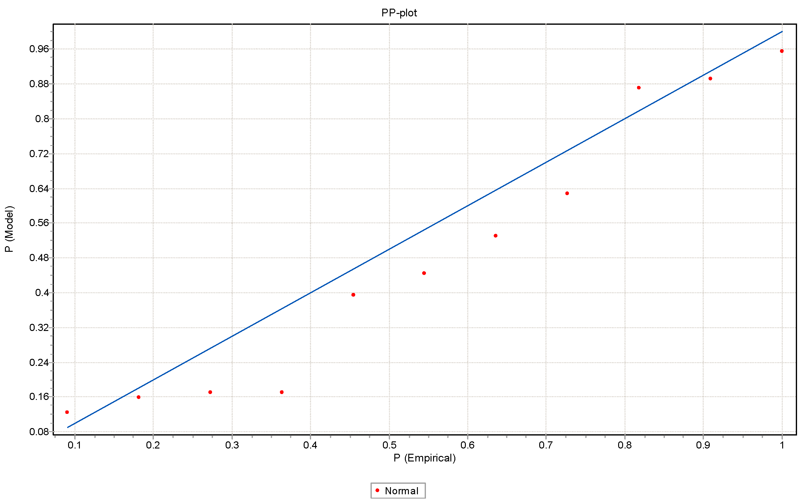
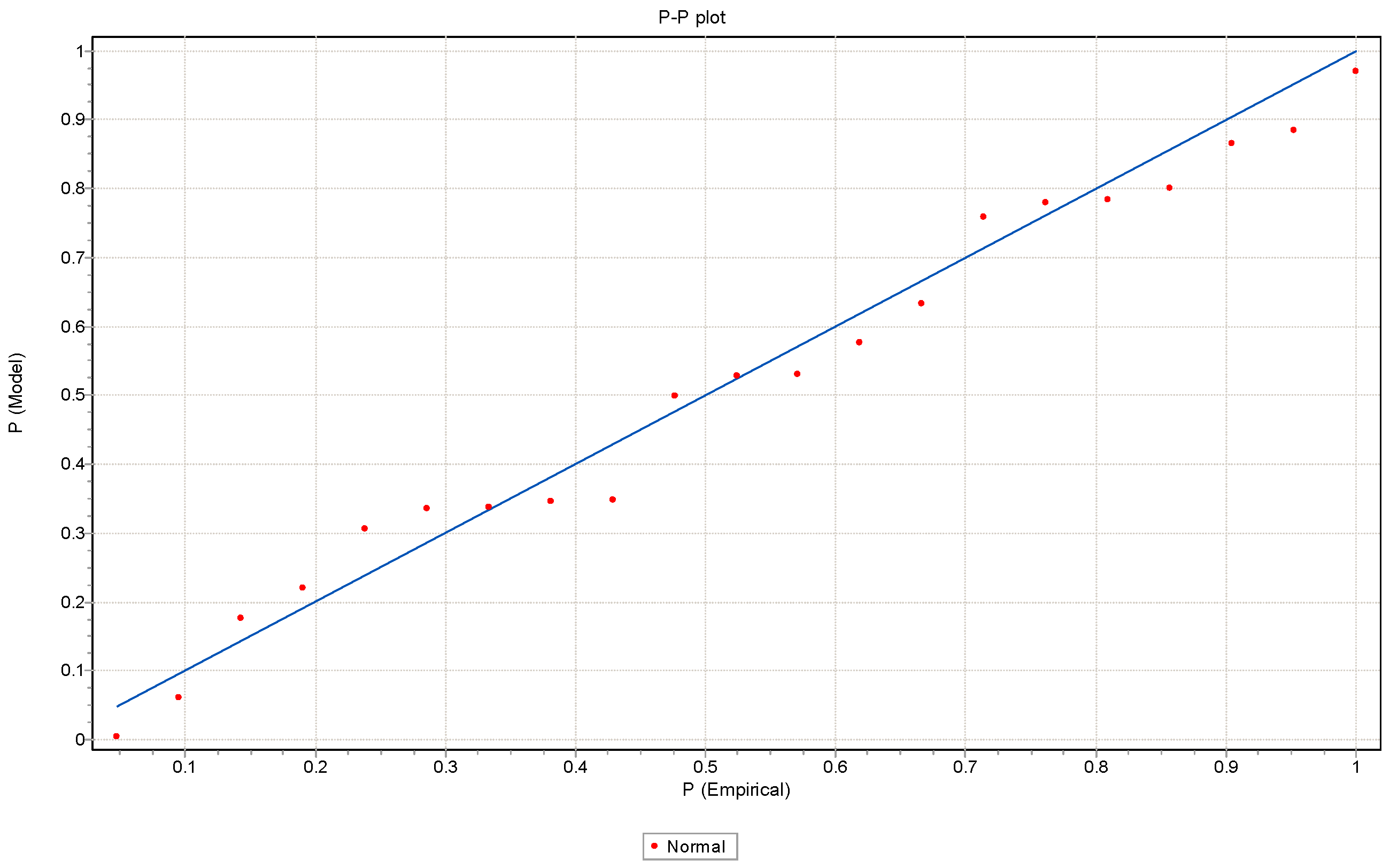
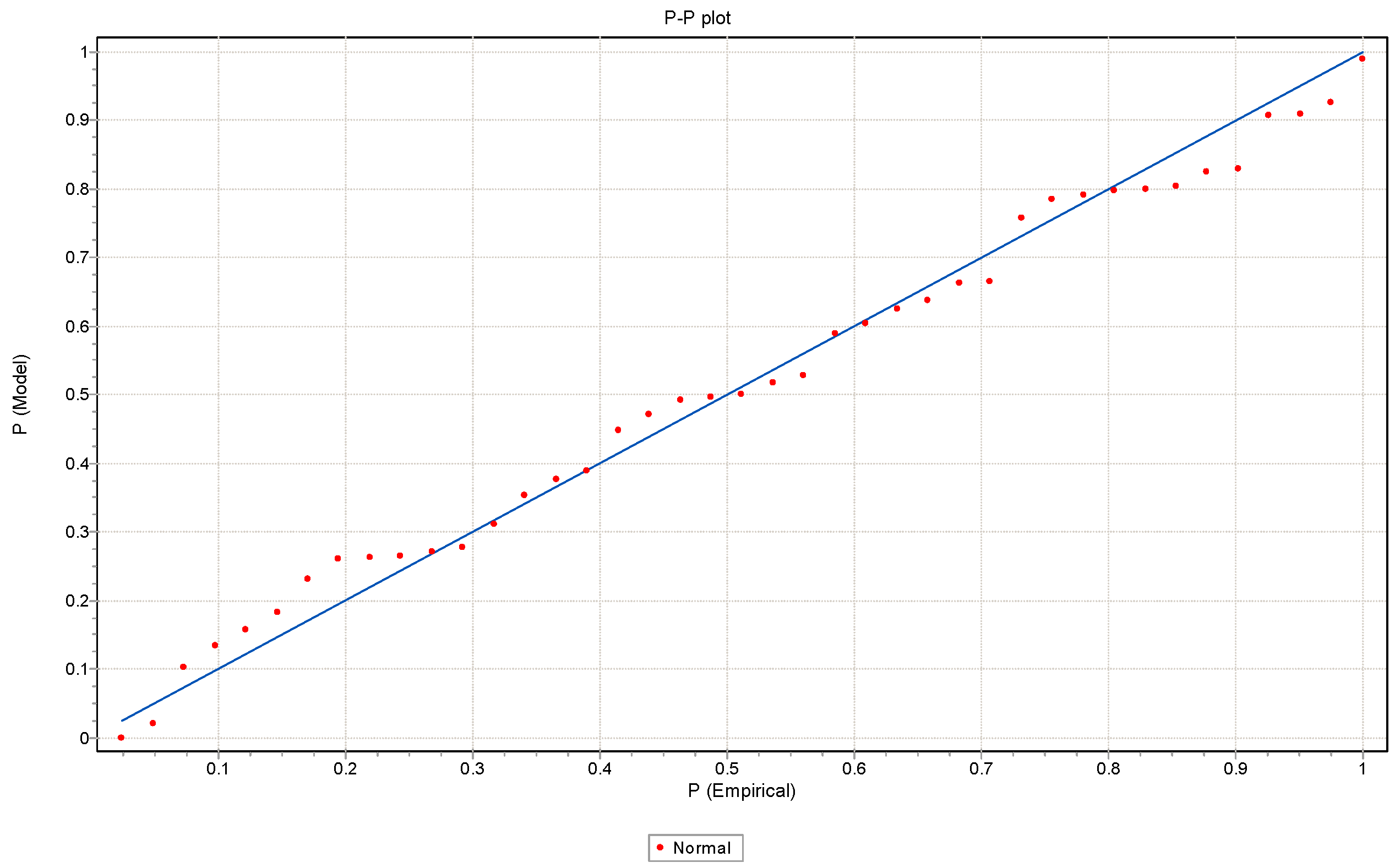
58]. We have conducted the A-D test on the average abnormal returns for each event windows E1, E2, and E3 proving the normality assumption. Graphically, we design the corresponding PP-plots (
Figure 1,
Figure 2 and
Figure 3):
In order to test the significance of cumulative abnormal returns we first apply the parametric
t-test. The traditional
t-test relies on the assumption that the abnormal returns are normally distributed
As the variance
is not known, the variance of the residuals obtained in the estimation period of the regression model is used as an estimator [
45].The null hypothesis is that stock prices do not respond to the event. Assuming that the abnormal returns are independent and identically distributed, the statistic follows a Student’s t-distribution under this hypothesis. For the average abnormal returns, the statistic is defined as:
Similarly, for the accumulated abnormal returns, the statistic is:
The null hypothesis is that the expected cumulative return is equal to zero. Furthermore, we also carried out two nonparametric tests. According to Campbell and Wasley [
59], the inclusion of nonparametric test checks the robustness of the conclusions based on the parametric test. In this particular case, we used the sign test [
46] and the Wilcoxon test [
60,
61]. The sign test is a binomial test, which calibrates if the frequency of abnormal positive residuals is equal to 50%. To implement this test, we should determine the proportion of values in the sample that shed no negative abnormal returns under the null hypothesis. The null value is calculated as the average fraction of stocks with no negative abnormal returns in the estimation period. If abnormal returns are independent, under the null hypothesis, the number of positive abnormal return values follows a binomial distribution with parameter
p, and the statistic is:
where
p0 reflects the observed proportion of positive returns in a given time window. This statistic is distributed as a normal law of variance 0 and mean 1.
The Wilcoxon test considers both the sign and the magnitude of abnormal returns, with the statistic:
where,
is the positive range of the absolute value of abnormal returns. This test assumes that none of the absolute values are the same and each is non-zero. Under the null hypothesis that the probability of positive and negative abnormal returns is equal, when
N is large,
W asymptotically follows a normal distribution with a mean and variance as follows, respectively:
Since adjusted abnormal returns are potentially more precise in capturing the reputational damage suffered by the firm responsible for the oil spill, we applied the same rationale to the raw , resulting in .
5. Main Findings and Results
Table 4 summarizes the results obtained in the parametric
t-test conducted on cumulative abnormal returns for the three event windows proposed above; E1 (−5, 5), E2 (−10, 10), and E3 (−20, 20).
For event window E1 (−5, 5), since the p-value is higher than our choice of significance (0.01, 0.05, 0.1), the null hypothesis is confirmed. In contrast, for event windows E2 (−10, 10) and E3 (−20, 20), the p-value is higher than the α-level, so the null hypothesis is rejected; in other words, the expected cumulated abnormal returns are significantly different from zero, which is an indication of abnormal returns around the date of the event.
In order to assess the robustness of the parametric t-test results, we have also applied two non-parametric tests: the sign test and the Wilcoxon test. The following tables illustrate the results:
The tables above show that the sign test (
Table 5) and the Wilcoxon test (
Table 6) offer similar results to the parametric
t-test: the null hypothesis is accepted in event window E1 (−5, 5), whereas in E2 (−10, 10) and E3 (−20, 20) it is rejected. CARs are shown to be statistically significant in windows E2 (−10, 10) and E3 (−20, 20). In other words, the hypothesis concerning the existence of abnormal returns on event day (
t = 0), as well as the days immediately before and after, are confirmed for event windows E2 (−10, 10) and E3 (−20, 20) at three α-levels (0.1, 0.05, 0.01).
In order to isolate the reputational effect, we now estimate the reputational cumulative abnormal returns
. CAR(Rep) is obtained by adding the loss ratio [
22] to abnormal returns on day 0. The loss ratio for each event is presented in
Table 7.
This time we exclusively focused on windows E2 (−10, 10) and E3 (−20, 20) because of their significance in the previous analysis. Similarly, we have also tested the statistical significance of
values by using a parametric
t-test. The
t-test confirmed that
values are significant for the selected event windows (E2, E3), at 10%, 5%, and 1% confidence levels;
p-values are (0.006) for E1, and (0.00) for E2 and E3, respectively. Moreover, results obtained in non-parametric tests are in accordance with the
t-test as the
Table 8,
Table 9 and
Table 10 illustrate:
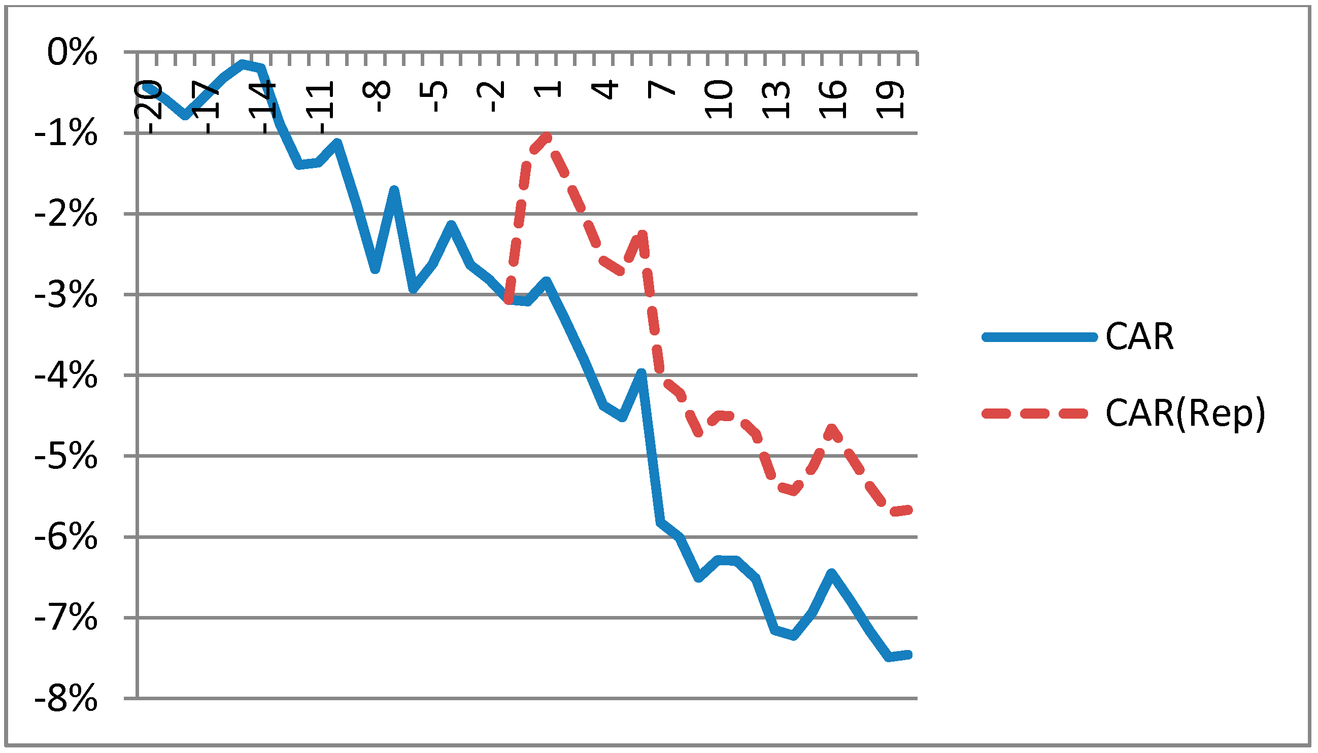
Once the statistical significance of
for the event windows E2 and E3 has been proved, the results were also plotted against raw
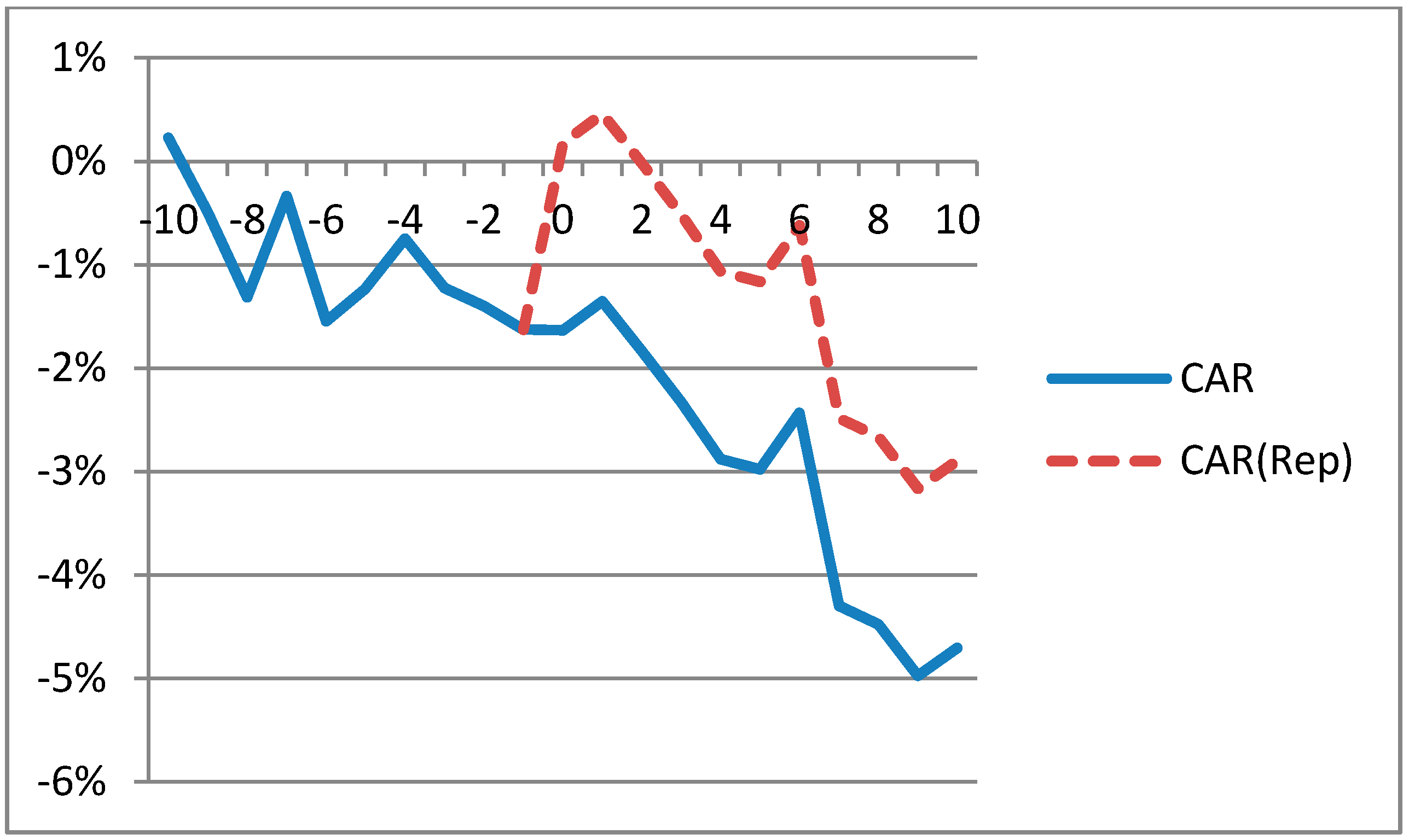
. The following charts illustrate the impact of operational losses separately from their effect on the firms’ reputations in both E2 and E3 event windows. In particular, the blue line in
Figure 4 reflects the strong market reaction to the media announcement of the oil spill by displaying the average value of cumulative abnormal returns (
) for the ten days before (−10) and after (+10) the disaster. In contrast, the red line represents the reputational effect, isolated by adjusting raw
with the loss ratio on day zero; that is, the average CAR(Rep) is calculated for the following ten days after the disaster.
values show a sharper negative trend and reach −5% on day (+10). Values do not bounce back until after ten days have passed since the announcement. Similarly,
Figure 5 shows the behavior of cumulative abnormal returns for the event window E3 (−20, +20). Mean cumulative abnormal returns are represented by the blue line, which indicates a decrease in stock market capitalization in the 20 days following the event. The figures show that
values decrease more in E3 (−20, +20) than in E2 (−10, +10); for instance, on day 0,
value for E2 is approximately −1.8%, while for E3 it is −3.1%. The reputational effect is even more striking for E3; while the reputational effect on day 0 even drops below −1%, for E2 the reputational effect does not emerge until two days later. Then, CAR(Rep) is higher for E3 (−20, +20) than E2 (−10, +10).
6. Conclusions
This study examines the impact of recent medium-sized and large oil spills on the reputation of US oil and gas companies listed on the NYSE, providing new insights about the estimation of reputational risk in non-financial firms. A standard short-horizon event study technique was implemented, and three different time windows, built around the day the spills were announced in the media, were taken into consideration. We aimed to highlight the negative responses of the stock market to oil spill disasters, even if the actual amounts lost are not known in detail. More specifically, our results reveal a significant negative impact on the stock prices of the companies analyzed; we also observed significant cumulative negative abnormal returns (CAR) around the event date, especially for event windows that were 21 and 41 days long. Moreover, we observed that the negative effect continues 10 and 20 days after the event. Therefore, a recovery is not ensuing in these time intervals. However, in the shortest event window (11 days), the abnormal returns are not as statistically significant as in the longest ones. This implies that reputational effects tied to oil spill disasters take time to be reflected significantly in terms of abnormal returns, that is, they are not as instant as expected. In this sense, financial perceptions on environmental disasters seem to be lagged with respect to the social perception on such announcements in the media.
On the other hand, by using an approximation of the loss ratio, we can not only identify the corporate reputational risk, but also isolate the impact of financial perceptions of such episodes on market returns by using the new metric CAR(Rep). Results are conclusive concerning the damage caused to a firm’s reputation by oil spill disasters. The effect is even more pronounced regarding the longest window (41 days), where mean cumulative abnormal reputational returns CAR(Rep) is particularly negative. Similarly, the reputational effect is also more pronounced in the longest event window. Reputational risk depends on the stakeholders’ financial perceptions that the company may incur losses in the future as a consequence of negligence, so it motivates managers to adopt better corporate environmental behavior and put more effort into controlling security and environmental hazards.


