Trend Prediction and Decomposed Driving Factors of Carbon Emissions in Jiangsu Province during 2015–2020

Abstract

According to the economic and energy consumption statistics in Jiangsu Province, we combined the GM (1, 1) grey model and polynomial regression to forecast carbon emissions. Historical and projected emissions were decomposed using the Logarithmic Mean Divisia Index (LMDI) approach to assess the relative contribution of different factors to emission variability. The results showed that carbon emissions will continue to increase in Jiangsu province during 2015–2020 period and cumulative carbon emissions will increase by 39.5487 million tons within the forecast period. The growth of gross domestic product (GDP) per capita plays the greatest positive role in driving carbon emission growth. Furthermore, the improvement of energy usage efficiency is the primary factor responsible for reducing carbon emissions. Factors of population, industry structure adjustment and the optimization of fuel mix also help to reduce carbon emissions. Based on the LMDI analysis, we provide some advice for policy-makers in Jiangsu and other provinces in China.

1. Introduction

Recently, the issue of climate change has been under increasing levels of scrutiny by governments and relevant stakeholders worldwide. The United Nations Intergovernmental Panel on Climate Change (IPCC) has released five assessment reports which analyzed the root causes of climate change and its effect on the planet in the years 1990, 1995, 2001, 2007, with the most recent in 2012. The literature on the subject overwhelmingly suggests that climate change is highly correlated to carbon emissions, and as a result the study of carbon emissions is of unparalleled significance under the background of climate change.

Lying on the eastern coast of mainland China, Jiangsu province (Jiangsu, hereafter), is one of the leading provinces in manufacturing electronics and apparel items. It has a gross domestic product (GDP) of 6.5 trillion yuan ($980 billion USD) in 2015, ranking second nationally. The annual fossil fuel energy consumption of Jiangsu also ranks very highly within the country. As is shown in Figure 1, energy consumption in Jiangsu rapidly increased from 2005–2014, the total amount of energy consumption remains high despite a declining growth rate. Although Jiangsu has advanced manufacturing capabilities and emission reduction technology, due to the construction of high-speed inter-city railways connecting 26 out of 44 counties and cities, it is estimated that the process for urbanization and industrialization of Jiangsu will be further accelerated resulting in increased energy demands and economic development-derived carbon emissions. Therefore, conducting a scientific analysis of the future trend of carbon emissions for Jiangsu and devising methods of emission reduction are of great importance.

The relationship between economic growth, energy consumption, and carbon dioxide emissions has been extensively analyzed over the past two decades. Kais [1] provided new empirical evidence to confirm that the Environmental Kuznets Curve (EKC) hypothesis, which was first defined by Simon Kuznets [2], posited an inverted U-shaped curve between economic growth and environmental degradation. Lau [3] indicated that good institutional quality is important in controlling carbon dioxide emissions in the process of economic development. The findings of Gallego-Álvarez [4] showed a reduction in emissions that generates a positive impact on financial performance, contributing to the literature on the relationship between carbon emission reduction and corporate performance.

Estimating and forecasting the amounts of carbon dioxide (CO₂) emitted into the atmosphere are crucial for planning and analyzing mitigation efforts and for development scenarios of future emissions. Burke [5] investigated carbon dioxide emissions from the combustion of fossil fuels and the manufacture of cement. The works of Tan [6] and Ertugrul [7] provided several extensive studies on the calculation of carbon emissions. A plausible method of computer modeling combining genetic algorithms and a chemical reactor network was developed by Christopher [8] to predict alternative fuel gaseous emissions. Multivariable regression analysis was merged with partial life cycle assessment (LCA) and building information modeling (BIM) for the prediction of environmental degradation within the housing sector [9]. However, forecasting results depended on statistical data, which change rapidly over time. The grey prediction model is an alternative forecasting tool for systems with complex, uncertain and chaotic structures because of their low data requirements to build forecasting models [10]. Initially proposed by Deng [11], the grey model (GM) was used to quantify uncertainty and information insufficiency. Following its proposal, the grey model has been used in various advanced applications. Wang [12] established a small-sample effective rolling GM (1, 1) model under eight different datasets to forecast future gas consumption. The metabolic grey model (MGM), metabolic residual-error grey model (MREGM), and the metabolic Markov-residual-error grey model (MMREGM) were proposed by Chen [13] and used to predict the capacity of lithium-ion batteries in relation to discharge cycles throughout their lifetimes. The GM (1, 1) model is currently one of the most widely used grey prediction models for predicting carbon emissions [14,15].

The index decomposition analysis (IDA) method has been widely applied to analyze factors influencing carbon emissions. IDAs are mainly divided into Laspeyres index decomposition and Divisia index decomposition analyses [16]. The LMDI method was introduced and developed by Ang [17], who concluded it to be the most preferred decomposition analysis due to its robustness, adaptability and transparency in the interpretation of results. Various studies have used LMDI to investigate carbon emissions at regional and national scales [18,19,20]. Wang [21] found that economic development was the largest factor of increasing carbon dioxide emissions through a modified production-theoretical decomposition analysis approach.

The analysis of carbon emission-related content previously described is applied in various industries and fields of research. The research scope refers to the nationwide level, provincial level, and urban areas. However many of the influencing factors, accounting methods, and emission performance are only targeted towards the past and cannot be used to predict future trends. In the recent National Climate Change Plan (2014–2020) published by the National Development and Reform Commission, the State Council confirmed that China would commit to reduce its CO₂ emissions per unit of GDP in 2020 by at least 40%–50% as compared to 2005, and it was considered as an indicator of economic development in long-term planning. In this paper, the decomposition analysis for carbon emission factors is focused on future economic development and the energy consumption trend of the province of Jiangsu. In order to meet the target of long-term emission reductions, all relevant statistical data are conducted using a grey prediction model and a method of LMDI decomposition has been applied to future emissions projections, which is aimed at describing future directions of emission reduction for Jiangsu and providing advice on the formulation of emission reduction policies for Jiangsu and other provinces with similar economic and environmental circumstances.

The rest of this paper is organized as follows: Section 2 presents the methodology and data; forecasting and decomposition results are put forward in Section 3; Section 4 provides a discussion of the results; and Section 5 gives the conclusion and puts forward advice based on the results of the analysis.

2. Methodology and Data

2.1. Data Source

The data used in the following study includes population, energy consumption data, and economic data, etc., which were obtained from the Regional Statistical Yearbook [22,23,24,25,26,27,28,29,30,31,32,33,34,35,36,37,38,39,40,41,42,43,44,45,46,47,48,49,50,51].

Population and economic data were collected from the Jiangsu Statistical Yearbook 2001–2015 [22,23,24,25,26,27,28,29,30,31,32,33,34,35]. Energy consumption data for each sector were extracted from the China Energy Statistical Yearbook 2001–2015 [35,36,37,38,39,40,41,42,43,44,45,46,47,48,49,50,51]. Energy consumption of Jiangsu was divided into three parts: primary, secondary, and tertiary industries. The types of fuels consumed by three industries included eight typical kinds: raw coal, cleaned coal, coke, gasoline, diesel, fuel oil, liquefied petroleum gas, and natural gas. For ease of calculations, we categorize these eight types of energy sources as coal, petroleum, and natural gas; and CO₂ emissions are calculated with the three aggregated fuels. Corresponding to the types of energy sources, this paper takes the mean values of raw coal, cleaned coal, and coke’s carbon emission coefficients as coal’s carbon emission coefficient, and the mean values of gasoline, diesel, fuel oil, and liquefied petroleum gas’ emission coefficients as oil’s carbon emission coefficient. Due to the small variation in the coal and petroleum energy source’s inter-source carbon emission coefficients, and the addition of this paper’s main study of the evolution of emission increases and structural composition, the aggregation essentially will not have an impact on the final conclusion. The CO₂ emission factors for the eight types of fuels and three reclassified types are summarized in

Table 1. Various fuel CO₂ emission factors (unit: kg/kgce).

Original Fuels	Factors	Aggregated Fuels	Factors
Raw Coal	0.7559	Coal	0.7889
Cleaned Coal	0.7559
Coke	0.8550
Gasoline	0.5538	Oil	0.56715
Diesel	0.5921
Fuel Oil	0.6185
Liquefied Petroleum Gas	0.5042
Natural Gas	0.4483	Natural Gas	0.4483

.

CO₂ emissions are calculated by the following equation:

$$C={\displaystyle {\sum }_i{e}_i}\times f_i\times k_i$$

(1)

where $e_i$ denotes the consumption of fuel i (unit: cubic meter for liquefied petroleum gas, and natural gas; kg for other fuels); $f_i$ is the standard coal coefficient used to convert the different types of energy to standard coal equivalents (SCE), which is derived from the General Principles of Comprehensive Energy Consumption Calculation (unit: kgce/cubic meter; kgce/kg); $k_i$ is the CO₂ emission factor for different types of fuels from the Guidelines on Provincial Greenhouse Gas Inventories.

2.2. GM (1, 1) Model

The algorithm of the GM (1, 1) grey prediction model can be summarized as follows:

Step 1: the non-negative time-sequence data X⁽⁰⁾ is expressed as:

$$X^{(0)}=\left\{x^{(0)}(1),x^{(0)}(2),\dots ,x^{(0)}(n)\right\}$$

(2)

where n ≥ 3.

Step 2: take accumulated generating operation (AGO) on X⁽⁰⁾ to weaken modulation tendencies:

$$X^{(1)}=\left\{x^{(1)}(1),x^{(1)}(2),\dots ,x^{(1)}(n)\right\}$$

(3)

where $x^{(1)}(n)={\displaystyle \sum _{k=1}^n{x}^{(0)}(k)}$.

Step 3: the basic form of GM (1, 1) is described by the following equation:

$$X^{(0)}(t)+a\cdot X^{(1)}(t)=u$$

(4)

where t denotes the independent variables in the system, a represents the developed coefficient, and u is the grey controlled variable. The model requires solutions for a and u.

Step 4: by using the ordinary least-square method, coefficient $\stackrel{⌢}{a}$ becomes:

$$\stackrel{⌢}{a}=\left[\begin{array}{l}a\\ u\end{array}\right]={\left(B^{T}B\right)}^{-1}{B}^T{Y}_n$$

(5)

where:

$$B=\left[\begin{array}{cccc}-\frac{1}{2}(x^{(1)}(1)+x^{(1)}(2))& 1& \cdots & 1\\ -\frac{1}{2}(x^{(1)}(2)+x^{(1)}(3))& 1& \cdots & 1\\ ⋮& 1& \cdots & 1\\ -\frac{1}{2}(x^{(1)}(n-1)+x^{(1)}(n))& 1& \cdots & 1\end{array}\right],\text{ and }{Y}_n={\left[x_1^{(0)}(2),x_1^{(0)}(3),\cdots ,x_1^{(0)}(n)\right]}^T;$$

Step 5: according to the estimated coefficients a and u, the response equation can be obtained:

$${\stackrel{⌢}{x}}^{(1)}(t+1)=(x^{(0)}(1)-\frac{u}{a})e^{-at}+\frac{u}{a}$$

(6)

Step 6: by performing inverse accumulated generating operation (IAGO) on ${\stackrel{⌢}{x}}^{(1)}$, the prediction value is produced:

$${\stackrel{⌢}{x}}^{(0)}(t+1)=-a\cdot (x^{(0)}(1)-\frac{u}{a})e^{-at}$$

(7)

or:

$${\stackrel{⌢}{x}}^{(0)}(t+1)={\stackrel{⌢}{x}}^{(1)}(t+1)-{\stackrel{⌢}{x}}^{(1)}(t)$$

(8)

To demonstrate the reliability of the GM (1, 1) model, the posterior variance test is used to discuss the results of fitting and prediction. Criteria of the posterior variance test include the indicators, posterior variance ratio C, and small error probability P.

The posterior variance ratio is defined as follows:

$$\mathrm{C}=\frac{S_2}{S_1}=\sqrt{\frac{{S_2}^2}{{S_1}^2}}$$

(9)

where ${S_2}^2=\frac{1}{m-1}{\displaystyle \sum _{t=1}^{m-1}}{({\epsilon }^{(0)}(t)-{\overline{\epsilon }}^{(0)}(t))}^2$, and ${S_1}^2=\frac{1}{m-1}{\displaystyle \sum _{t=1}^m(x^{(0)}(t)}-{\overline{x}}^{(0)}(t){)}^2$.

${\epsilon }^{(0)}(t)$ represents the residual between the predicted value ${\stackrel{⌢}{x}}^{(0)}(t)$ and the actual value $x^{(0)}(t)$ at time t.

Small error probability P is expressed as $\mathrm{P}=\left\{\left|{\epsilon }^{(0)}(t)-{\overline{\epsilon }}^{(0)}(t)\right|<0.6745S_1\right\}$. The range of indicator values C and P is such that: C > 0, 0 ≤ P ≤ 1, where P > 0.95 and C < 0.35 indicates a highly accurate forecast, P > 0.60 and C < 0.80 indicates a reasonable forecast, and P < 0.60 and C > 0.80 indicates an unreasonable range.

2.3. Polynomial Regression Analysis

Polynomial regression analysis is a powerful statistical tool for estimating relationships between variables, which has many applications in different areas, such as engineering, the environmental sciences, finance, and economics. It can be summarized by the following steps:

(1)

Determine the number of polynomials by observing the changing trend of the actual data.

(2)

Transform the general polynomial $y=a_0+a_{1}x+a_2{x}^2+\cdots +a_m{x}^m$ into a linear function $y=a_0+a_1{z}_1+a_2{z}_2+\cdots +a_m{z}_m$, where $z_1=x,z_1=x^2,\cdots ,z_m=x^m$.

(3)

Estimate the parameters $a_0,a_1,a_2,\cdots ,a_m$ by using the ordinary least-square method.

(4)

Calculate the predicted values with the estimated multivariate linear function.

2.4. LMDI Decomposition Model

The LMDI decomposition approach is widely used in studies of environment and energy problems. A practical guide to Log-Mean Divisia Index Method I (LMDI-I ) is given by Ang [17]. Changes in CO₂ emissions from industry may be studied by quantifying the contributions the variability of six different factors: population, GDP (PPP) per capita, industrial activity mix, energy intensity, fuel mix, and CO₂ emission factors. The subcategories of the aggregate are the industrial sectors and fuel types. The decomposition analysis problem can be formulated either additively or multiplicatively. In multiplicative decomposition, we decompose the CO₂ emissions changes into the following factors:

$$C={\displaystyle \sum _{i=1}^m{\displaystyle \sum _{j=1}^n\frac{C_{ij}}{E_{ij}}}}\times \frac{E_{ij}}{E_i}\times \frac{E_i}{G_i}\times \frac{G_i}{G}\times \frac{G}{R}\times R={\displaystyle \sum _{i=1}^m{\displaystyle \sum _{j=1}^n{k}_{ij}\times n_{ij}\times e_i\times s_i\times w\times r}}$$

Variable definitions are summarized in

Table 2. Definitions of variables.

Variables	Definitions	Unit
R	Population	1.0 × 104 persons
G	GDP	1.0 × 108 yuan
Gi	GDP of industrial sectors	1.0 × 108 yuan
Ei	Gross energy consumption of industrial sectors	1.0 × 104 tce
Eij	Consumption of fuel j in industrial sector i	1.0 × 104 tce
Cij	CO2 emissions arising from fuel j in industrial sector i	1.0 × 104 tons
r	Population size	1.0 × 104 persons
w	GDP per capita	yuan/person
si	Share of GDP of industrial sector i	Percentage point
ei	Energy intensity in industrial sector i	tce/1.0 × 104 yuan
nij	Fuel mix (share of consumption of fuel j in gross Energy consumption in industrial sector i)	Percentage point
kij	CO2 emission coefficient: CO2 emission per unit of Fuel j in industrial sector i	1.0 × 104 tons

.

In additive decomposition, we decompose the increased carbon emissions:

$$\Delta C=\Delta C_r+\Delta C_w+\Delta C_s+\Delta C_e+\Delta C_n+\Delta C_k$$

Similar to some related studies, because CO₂ emission coefficients of various energy sources are all assumed to be fixed when calculating CO₂ emissions, the term ΔC_k in the equation does not contribute to CO₂ emission variability and has a value of zero. Hence, the final drivers of CO₂ emission variability are decomposed into five corresponding factors:

$$\Delta C=\Delta C_r+\Delta C_w+\Delta C_s+\Delta C_e+\Delta C_n$$

where $\Delta C_r$ denotes the CO₂ increase or decrease increments as caused by a change in population; $\Delta C_w$ is the increment of CO₂ emissions caused by change of GDP per capita; $\Delta C_s$ is the increment of CO₂ emissions caused by changes in industrial structure, which is represented by a share of GDP in the industrial sector i; $\Delta C_e$ is the increment of CO₂ emissions caused by changes in energy intensity; and $\Delta C_n$ is the increment of CO₂ emissions caused by change in the proportion of energy consumption. The LMDI formulae are summarized in

Table 3. The LMDI formulae.

Additive Decomposition
Change Scheme	LMDI Formulae
$\Delta C=\Delta C_r+\Delta C_w+\Delta C_s+\Delta C_e+\Delta C_n$	$\Delta C_r={\displaystyle \sum _{i=1}^m{\displaystyle \sum _{j=1}^n(\frac{C_{ij}^{t+1}-C_{ij}^t}{\text{ln}{C}_{ij}^{t+1}-\text{ln}{C}_{ij}^t})}}\times \text{ln}(\frac{r(t+1)}{r(t)})$
	$\Delta C_w={\displaystyle \sum _{i=1}^m{\displaystyle \sum _{j=1}^n(\frac{C_{ij}^{t+1}-C_{ij}^t}{\text{ln}{C}_{ij}^{t+1}-\text{ln}{C}_{ij}^t})}}\times \text{ln}(\frac{w(t+1)}{w(t)})$
	$\Delta C_s={\displaystyle \sum _{i=1}^m{\displaystyle \sum _{j=1}^n(\frac{C_{ij}^{t+1}-C_{ij}^t}{\text{ln}{C}_{ij}^{t+1}-\text{ln}{C}_{ij}^t})}}\times \text{ln}(\frac{s_i(t+1)}{s_i(t)})$
	$\Delta C_e={\displaystyle \sum _{i=1}^m{\displaystyle \sum _{j=1}^n(\frac{C_{ij}^{t+1}-C_{ij}^t}{\text{ln}{C}_{ij}^{t+1}-\text{ln}{C}_{ij}^t})}}\times \text{ln}(\frac{e_i(t+1)}{e_i(t)})$
	$\Delta C_n={\displaystyle \sum _{i=1}^m{\displaystyle \sum _{j=1}^n(\frac{C_{ij}^{t+1}-C_{ij}^t}{\text{ln}{C}_{ij}^{t+1}-\text{ln}{C}_{ij}^t})}}\times \text{ln}(\frac{n_{ij}(t+1)}{n_{ij}(t)})$

where m represents the types of industry, n represents the types of energy, and t represents the year.

3. Results

3.1. Forecasting Results

In the primary industry, natural gas consumption remained zero over the past 15 years, and it is less likely to be consumed on a large scale in the future. As a result, it is assumed that the consumption is still zero in the forecast period. To better evaluate the performance of the GM (1, 1) model, indicator values C and P are calculated and the model evaluation results are given in

Table 4. GM (1, 1) model evaluation results.

Prediction Terms	C Value	P Value
Population	0.1536	1.0000
Primary Industry GDP	0.1351	1.0000
Secondary Industry GDP	0.1511	1.0000
Tertiary Industry GDP	0.0795	1.0000
Primary Industry Coal Consumption	0.3891	1.0000
Primary Industry Oil Consumption	0.4019	0.9333
Primary Industry Natural Gas Consumption	model is not suitable for prediction
Secondary Industry Coal Consumption	0.4185	1.0000
Secondary Industry Oil Consumption	0.3208	0.8889
Secondary Industry Natural Gas Consumption	1.4430	0.3333
Tertiary Industry Coal Consumption	0.6940	0.7333
Tertiary Industry Oil Consumption	0.2309	1.0000
Tertiary Industry Natural Gas Consumption	1.4464	0.3333

.

In accordance with the optimum range of indicator values C and P, as previously mentioned, most of the model produced very good estimates except for secondary industry natural gas consumption and tertiary industry natural gas consumption. Those two terms were predicted by the polynomial regression model. Results are shown in

Table 5. Evaluation results of polynomial regression analysis.

Prediction Terms	Prediction Model	Adjusted R2
Secondary Industry Natural Gas Consumption	Y = −0.202X3 + 8.639X2 − 32.021X + 27.044	R2 = 0.9906
Tertiary Industry Natural Gas Consumption	Y = −0.22X3 + 1.387X2 − 9.005X + 11.305	R2 = 0.9054

.

The prediction results of the above factors are shown in

Table 6. Prediction results.

Prediction Terms	Unit	2015	2016	2017	2018	2019	2020
Population	/10,000 persons	8079.24	8130.83	8182.75	8234.99	8287.58	8340.50
Primary Industry GDP	1.0 × 108 RMB	4301.58	4773.69	5297.61	5879.04	6524.27	7240.33
Secondary Industry GDP	1.0 × 108 RMB	39,486.8	44,824.1	50,882.8	57,760.5	65,567.9	74,430.5
Tertiary Industry GDP	1.0 × 108 RMB	39,193.4	46,392.8	54,914.8	65,502.2	76,492.5	91,076.2
Primary Industry Coal Consumption	1.0 × 104 tce	35.10	34.09	33.11	32.16	31.23	30.33
Primary Industry Oil Consumption	1.0 × 104 tce	358.61	383.63	410.41	439.05	469.69	502.47
Primary Industry Natural Gas Consumption	1.0 × 104 tce	0	0	0	0	0	0
Secondary Industry Coal Consumption	1.0 × 104 tce	8865.8	9563.3	10,315.5	11,127.0	12,002.3	12,946.5
Secondary Industry Oil Consumption	1.0 × 104 tce	371.87	348.84	327.23	306.96	287.95	270.11
Secondary Industry Natural Gas Consumption	1.0 × 104 tce	896.88	984.51	1068.77	1148.44	1222.29	1289.13
Tertiary Industry Coal Consumption	1.0 × 104 tce	21.32	20.36	19.45	18.58	17.75	16.96
Tertiary Industry Oil Consumption	1.0 × 104 tce	1908.72	2068.22	2241.04	2428.31	2631.23	2851.11
Tertiary Industry Natural Gas Consumption	1.0 × 104 tce	132.05	150.82	170.12	189.81	209.76	229.85

.

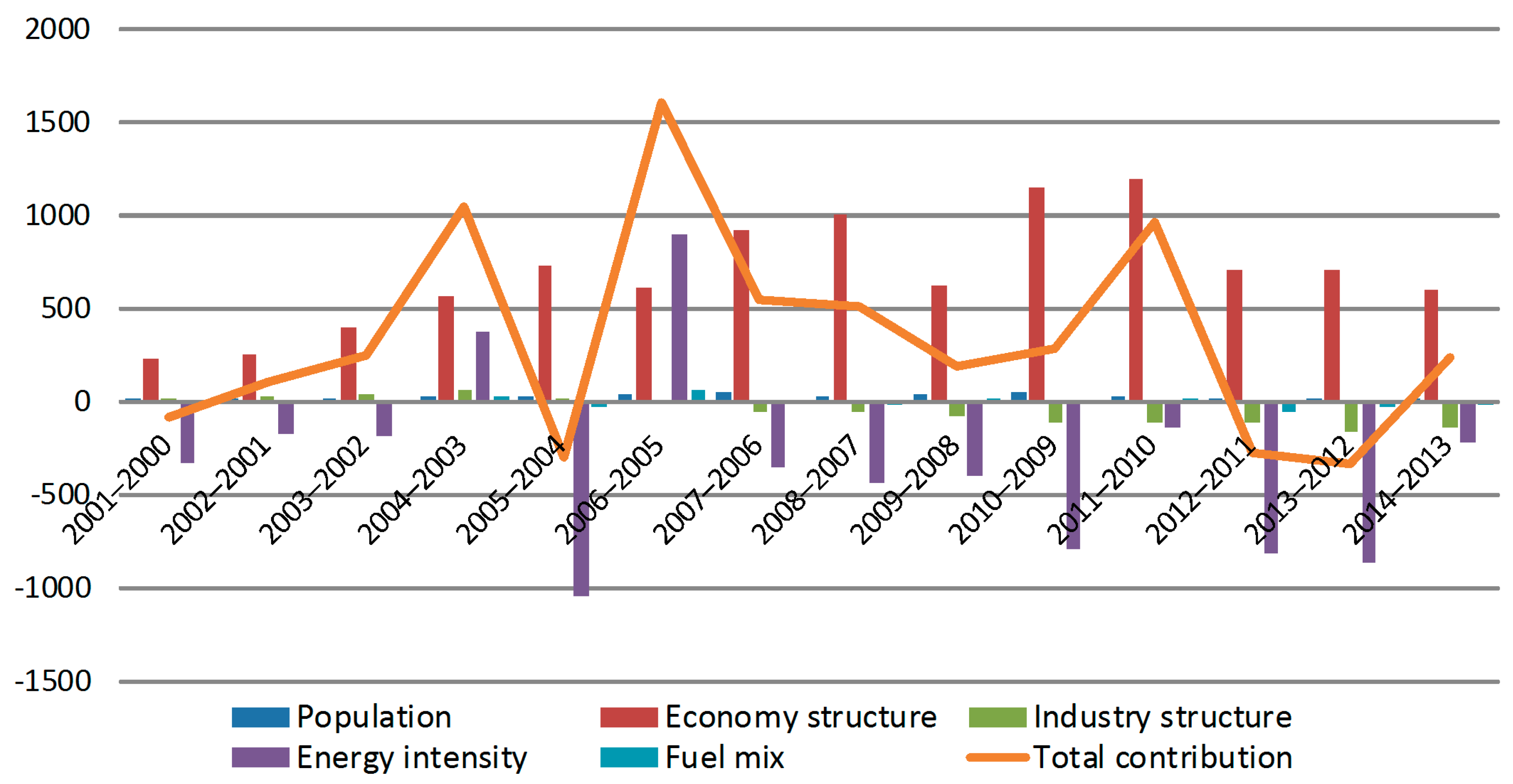
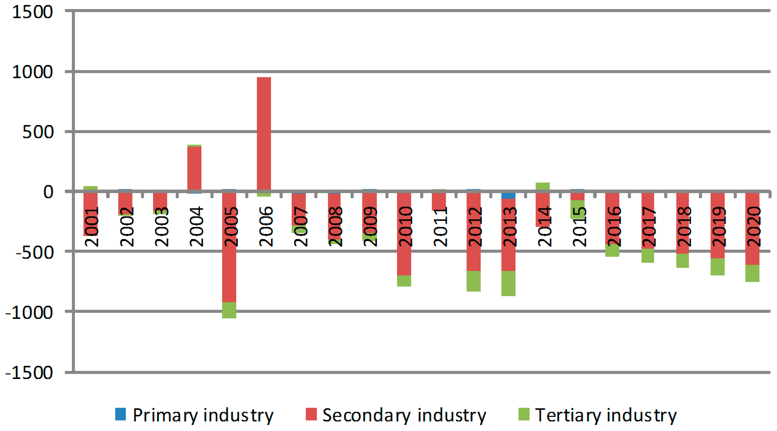
3.2. LMDI Decomposition Results

Table 7. Decomposition of the CO₂ emissions from 2000–2014 (unit: 10,000 tons).

Year	Population	Economy Structure	Industry Structure	Energy Intensity	Fuel Mix	Total Contribution
2001–2000	10.11	228.10	0.52	−326.77	−4.00	−92.04
2002–2001	15.17	258.33	23.93	−181.72	−6.65	109.06
2003–2002	17.99	390.85	43.72	−190.45	−12.64	249.46
2004–2003	27.73	567.95	56.64	370.05	21.67	1044.04
2005–2004	30.68	732.04	11.69	−1045.57	−29.47	−300.64
2006–2005	36.84	613.55	−8.00	896.50	60.10	1598.97
2007–2006	47.14	917.56	−59.39	−353.43	−6.93	544.95
2008–2007	29.92	997.84	−58.91	−437.24	−18.05	513.55
2009–2008	38.33	625.59	−79.54	−404.40	8.46	188.43
2010–2009	49.02	1149.17	−121.51	−789.77	−3.12	283.79
2011–2010	26.68	1188.22	−112.33	−142.57	4.15	964.15
2012–2011	20.11	700.65	−116.01	−824.69	−53.40	−273.35
2013–2012	17.75	704.92	−162.01	−865.38	−37.55	−342.27
2014–2013	18.58	595.54	−136.42	−225.31	−16.22	236.16
Total	386.04	9670.29	−717.64	−4520.76	−93.65	4724.28

shows CO₂ emissions and the contribution of the various factors from 2000–2014.

Table 7 reflects the decomposition of increased carbon emissions. The combined effect on carbon emissions was 47.2428 million tons between the years of 2000–2014. Between the years 2000–2014, population, changes in industrial structure, economic structure, energy intensity, and energy structure contributed 3.8604 million tons, 96.7029 million tons, −7.1764 million tons, −45.2076 million tons, and −936.5 thousand tons to carbon emissions, respectively. Negative values of total contribution indicate reduced carbon emissions as compared to the previous year. Except for years 2000, 2004, 2011, and 2012, carbon emissions in other years continued to rise. Based on the LMDI decomposition approach, we can identify the extent to which the total changes of these influencing factors contributed to the total growth of carbon emissions. As is shown in Figure 2, among those factors, economic structure played the greatest positive role in increasing carbon emissions, and energy intensity is the key factor for reducing carbon emissions. The remaining three factors, population, industrial structure, and fuel mix, have limited effects.

According to the decomposition results in

Table 8. Decomposition of CO₂ emissions from 2015–2020 (unit: 10,000 tons).

Year	Population	Economy Structure	Industry Structure	Energy Intensity	Fuel Mix	Total Contribution
2016–2015	59.69	1306.05	−131.46	−545.84	−16.54	671.90
2017–2016	64.26	1410.97	−146.14	−591.58	−10.11	727.40
2018–2017	69.15	1524.03	−162.27	−641.26	−2.87	786.79
2019–2018	74.41	1645.81	−179.97	−695.01	5.12	850.36
2020–2019	80.05	1776.93	−199.38	−752.97	13.79	918.43
Total	347.57	7663.80	−819.23	−3226.66	−10.61	3954.87

, cumulative carbon emissions will increase by 39.5487 million tons during the forecast period. Economic growth will still be the main driving force and variability in energy intensity will be the main constraint in the growth of carbon emissions.

4. Discussion

4.1. Economic Factors Analysis

As is easily seen in Table 7, throughout the years 2000–2010, the effect of economic growth on rising carbon emissions in Jiangsu Province is positive and has a rising trend. Since 2011, the contribution of economy structure has experienced a declining trend in increasing CO₂ emissions. This result conforms with the fact that the economic growth slowed down during China’s ‘Twelfth Five Year Plan’ period (2011–2015), as compared to the ‘Eleventh Five Year Plan’, where the economy underwent a significant surge. Due to the global economic depression, China’s domestic economic development entered a new state of normalcy. In the complex global political and economic environment, Jiangsu actively promoted the optimization and upgrading of industrial structure. The province has maintained a stable rate of rapid growth under the relatively large stress of economic depression. Following the optimization of the industrial structure and the recovery of the global economy it is predicted that, within the estimation period, the contribution of Jiangsu’s economic structure will continue an upwards trend. As seen in Table 8, the overall increase in carbon emission caused by economic factors will be 76.6380 million tons, which then leads to the conclusion that, in curbing carbon emissions, a path of reducing economic growth must be taken. Though Jiangsu has made great contributions to the China’s economic development over the years, and the regional GDP is ranking at the forefront, there exists a great disparity between residential living standards and civil construction. In the near future, the task of developing the economic situation and improving residential living standards will continue to exist, while the economic growth speed of Jiangsu will not undergo a significant decrease. Thus, it can be seen that, with respect to Jiangsu, it is not enough to only rely on the control of economic growth for emission reduction; what is more important is to cooperate with other emission reduction-related affairs.

4.2. Energy Intensity Factor Analysis

Energy intensity is the ratio of energy consumption divided by GDP, which shows energy usage efficiency. As Table 7 shows, the energy intensity has little contribution to carbon emission increase within the period of 2000–2014. The result reveals that the energy efficiency has improved significantly and has contributed greatly to reducing carbon emissions. As shown in Figure 3, the three major industries’ contributions to the energy intensity are essentially negative; moreover, the largest negative contribution came from the secondary industry. The contribution to energy intensity from the primary industry remained constant, and the value of negative contribution every year is minor. The reason for this might be that the size of the primary industry is very small and, by taking this into consideration, the future devotion to the improvement of the secondary industry energy intensity should be given.

With the vigorous promotion of energy-conserving and emission-reducing equipment and technology, it is estimated that the energy efficiency for Jiangsu will continually increase as energy intensity decreases. Macroeconomic control that is mainly focused on energy conservation and emission reduction policies will be strengthened. The effect from earlier emission reduction policies will gradually bear fruit and, as shown in Table 8, during the time of forecasting data, energy intensity is still a main factor in curbing carbon emission growth.

4.3. Industrial Structure Factor Analysis

According to the value of the contribution from the industrial structure on carbon emissions varying in Table 7 above, the historical data can be divided into two stages:

(1)

Covering a period of 2000–2005, the effect on carbon emission amount from the industrial structure fluctuates and the absolute value is small. Therefore, the change of the industrial structure has a limited restricting effect on carbon emissions.

(2)

During the period of 2006–2014, the absolute value of contributions from the industrial structure on emission reduction has increased, which obviously shows trend of carbon emission reduction.

During the study estimation period, adjustments to the industrial structure had an obvious increasingly restrictive effect on carbon emission growth. As seen from Table 8, the absolute value of the industrial structure’s yearly contribution rose. From

Table 9. Incremental effects of industrial structure from 2015–2020 (unit: 10,000 tons).

Year	Primary Industry	Secondary Industry	Tertiary Industry	Total Effects
2016–2015	−9.86	−149.47	27.87	−131.46
2017–2016	−10.57	−165.12	29.55	−146.14
2018–2017	−11.33	−182.24	31.30	−162.27
2019–2018	−12.15	−200.95	33.13	−179.97
2020–2019	−13.05	−221.37	35.04	−199.38
Average	−11.39	−183.83	31.38	−163.85

it can be shown that, in the future, the secondary industry in Jiangsu will play an important role in emission reductions. The tertiary industry will increase its amount of the carbon emissions. Calculations demonstrate that, during the period of estimation, total input averages of the secondary and tertiary industries were 45% and 50%, respectively. Furthermore, the average annual contribution of energy intensity on carbon emissions for secondary and tertiary industries, respectively, are −1.8383 million tons and 313,800 tons. Therefore, the slightly lower proportion of the secondary industry output will result in good emission reductions. Though the proportion of tertiary industry increased every year, there were limited effects on carbon emissions. In the future, Jiangsu will continue the trend of transforming itself from higher proportions of secondary industries to tertiary ones, and this will have a great effect on emission reductions.

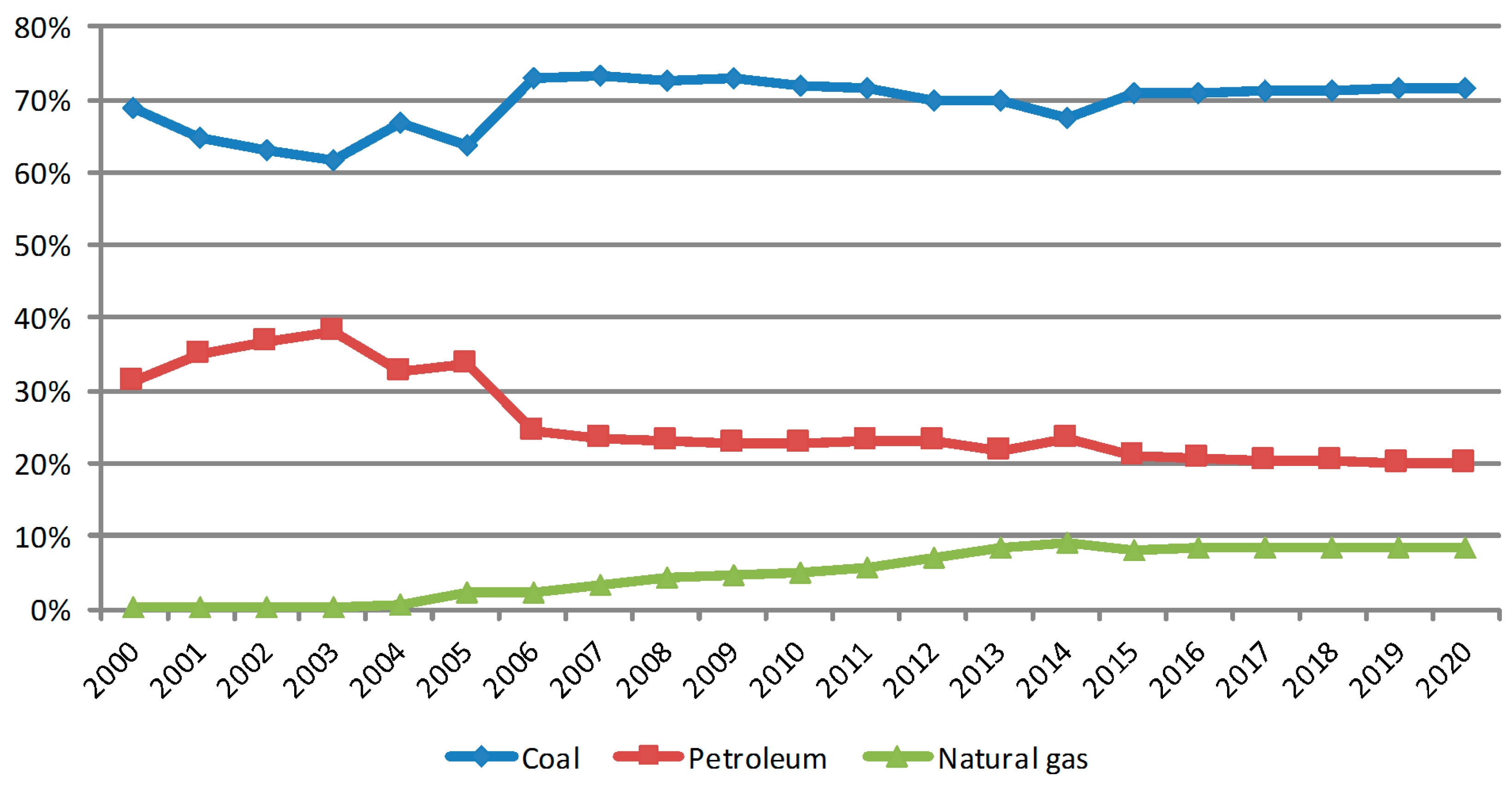
4.4. Energy Structure Factor Analysis

As seen from historical data, there is a slight effect of the energy consumption structure on carbon emissions which then leads to the proposition that energy structure composition has a relatively small influence on carbon emissions. Generally speaking, adjusting the energy structure would have an unstable and limited effect on carbon emission reductions. Starting in 2003, it can be shown that the energy structure had made positive contributions to carbon emissions. As Figure 4 illustrates, perhaps there was a decline in the ratio of petroleum consumption, which was accompanied by a gradual increase in the ratio of natural gas consumption. Lending credence to this hypothesis, the ratio of petroleum consumption decreased from 38% in 2003 to 24% in 2014 and, also as a result of the implementation of a west-east transmission of natural gas policy, the ratio of natural gas consumption increased to 9% from 2.31% in 2005. During the estimation period, adjustments of energy structures does not have an obvious effect on the restriction of increasing carbon emission growth; however, this effect is gradually disappearing. The reason for this is that the proportion of coal consumption was not significantly lowered. As is shown in Table 6, estimation data of the three major industries (primary, secondary, and tertiary) shows that the demand for coal grows daily. When energy consumption categories in Jiangsu are mostly comprised of coal, petroleum, and natural gas, small changes in the energy structure does not have a great effect on carbon emission reduction. With regard to energy sources, future strategies of emission reduction in this province must increasing rely on energy utilization efficiency.

4.5. Demographic Factors Analysis

As seen from historical data, the effect on carbon emission from demographic factors is stable, and changes in numerical values are not obvious. In recent years, Jiangsu was faced with the problem of rapid increases in population size and, for some cities, floating populations, i.e., the part of the population which resides in an area for a certain amount of time and for an array of reasons, but are not generally considered during an official census exercise, have exceeded the actual long-term/permanent resident population. Urbanization has consumed a lot of building materials and energy while, at the same time, people’s consumption habits have also significantly changed. All of these factors will contribute to increasing levels of energy consumption and, correspondingly, carbon emissions. According to model decomposition, it was found that population growth will lead to more carbon emissions during the period of 2015–2020. The absolute value of carbon emission caused by demographic factors is not large, but it ranks second only to economic factors. As Table 7 shows, the effect on carbon emissions from demographic factors is expected to be up to 3.4757 million tons from 2015–2020.

5. Conclusions and Suggestions

5.1. Conclusions

In this research, a grey prediction model combined with a polynomial regression model was applied to calculate future carbon emissions from 2015–2020. Based on historical and predicted carbon emissions, we used the LMDI decomposition model to analyze the contributions of different factors to changing carbon emissions in Jiangsu. We aimed at discussing the future direction of emission reduction for Jiangsu and providing advice on the formulation of emission reduction policies not only for the province studied in this work, but for other provinces of similar socioeconomic backgrounds.

From the analysis we can conclude that:

(1)

During the period of 2015–2020, the carbon emission of Jiangsu Province will increase at a constant pace.

(2)

Rapid economic growth is the main driving force that results in increasing carbon emissions. Energy intensity is the key factor for reducing carbon emissions. The results are consistent with the conclusion of the literatures [6,18,21].

(3)

Changes in the level of population size and structure, as well as industrial and energy-consumption structures, will also affect carbon emissions.

(4)

It is very likely that Jiangsu province will achieve a decrease of 40%–50% in CO₂ emissions per unit of GDP in 2020 as compared to the 2005 target. According to the prediction results, the population will increase to 83.4 million in 2020 from 75.88 million in 2005; total GDP of the three industries (primary, secondary, tertiary) will be 17,274.7 billion yuan ($2.6044 trillion, USD); and carbon emissions will reach 130.4 million tons per year. Under such circumstances, the CO₂ emissions per unit of GDP of the primary, secondary, and tertiary industry in 2020 will decrease by 55.11%, 42.96%, and 75.2%, respectively, as compared to 2005.

5.2. Suggestions

According to the conclusions made, the following advice for Jiangsu province and other provinces with similar situations is put forward:

(1)

The economic growth speed of Jiangsu will not undergo a significant decrease in the short term. Thus, it can be seen that with respect to Jiangsu, it is not enough to only rely on the control of economic growth for emission reduction; what is more important is to cooperate with other emission reduction related affairs.

(2)

As energy intensity is the key factor for reducing carbon emissions, it is necessary for enterprises to improve energy utilization efficiency. In terms of the energy consumption structure of Jiangsu, enterprises should be encouraged to control the rate of raw coal consumption and total energy consumption, and promote the usage of natural gas or other clean energies. Furthermore, as the largest negative contribution of the energy intensity factor comes from the secondary industry, it is suggested that the adjustments and upgrades of the industrial structure should be adhered to and new environmental protection technologies should be used to transform existing industrial enterprises.

(3)

As the transformation process of development centers changes to the tertiary industry, focus should be paid to the carbon emission of the tertiary industry, for there is a great need for energy in some parts of the tertiary industry, such as the catering and transportation industries. Therefore, the adjustment of the industrial structure should not only be focused on reducing the proportion off secondary industries, but the characteristics of the tertiary industry should also be considered.

(4)

It is essential for each city to revise original policies to meet long-term emission reduction targets, and pay attention to the industry that can achieve low- or zero-emissions in all stages of their life cycles.

References

1. Kais, S.; Sami, H. An econometric study of the impact of economic growth and energy use on carbon emissions: Panel data evidence from fifty eight countries. Renew. Sustain. Energy Rev. 2016, 59, 1101–1110. [Google Scholar] [CrossRef]
2. Kuznets, P.; Simon, P. Economic growth and income inequality. Am. Econ. Rev. 1955, 45, 1–28. [Google Scholar]
3. Lau, L.S.; Choong, C.K.; Eng, Y.K. Carbon dioxide emission, institutional quality, and economic growth: Empirical evidence in Malaysia. Renew. Energy 2014, 68, 276–281. [Google Scholar] [CrossRef]
4. Gallego-Álvarez, I.; Segura, L.; Martínez-Ferrero, J. Carbon emission reduction: The impact on the financial and operational performance of international companies. J. Clean. Prod. 2014, 103, 149–159. [Google Scholar] [CrossRef]
5. Burke, P.J.; Shahiduzzaman, M.; Stern, D.I. Carbon dioxide emissions in the short run: The rate and sources of economic growth matter. Glob. Environ. Chang. 2015, 33, 109–121. [Google Scholar] [CrossRef]
6. Tan, X.; Dong, L.; Chen, D.; Gu, B.; Zeng, Y. China’s regional CO2, emissions reduction potential: A study of Chongqing city. Appl. Energy 2016, 162, 1345–1354. [Google Scholar] [CrossRef]
7. Ertugrul, H.M.; Cetin, M.; Seker, F.; Seker, F.; Dogan, E. The impact of trade openness on global carbon dioxide emissions: Evidence from the top ten emitters among developing countries. Ecol. Indic. 2016, 67, 543–555. [Google Scholar] [CrossRef]
8. Leong, C.C.; Blakey, S.; Wilson, C.W. Genetic Algorithm optimised Chemical Reactors network: A novel technique for alternative fuels emission prediction. Swarm Evol. Comput. 2015, 27, 180–187. [Google Scholar] [CrossRef]
9. Gardezi, S.S.S.; Shafiq, N.; Zawawi, N.A.W.A.; Khamidi, M.F.; Farhan, S.A. A multivariable regression tool for embodied carbon footprint prediction in housing habitat. Habitat Int. 2016, 53, 292–300. [Google Scholar] [CrossRef]
10. Pao, H.T.; Fu, H.C.; Tseng, C.L. Forecasting of CO2, emissions, energy consumption and economic growth in China using an improved grey model. Energy 2012, 40, 400–409. [Google Scholar] [CrossRef]
11. Deng, J.L. Control problems of Grey system. Syst. Contr. Lett. 1982, 1, 288–294. [Google Scholar]
12. Wang, J.; Jiang, H.; Zhou, Q.; Wu, J.; Qin, S. China’s natural gas production and consumption analysis based on the multicycle Hubbert model and rolling Grey model. Renew. Sustain. Energy Rev. 2016, 53, 1149–1167. [Google Scholar] [CrossRef]
13. Chen, L.; Lin, W.; Li, J.; Tian, B.; Pan, H. Prediction of lithium-ion battery capacity with metabolic grey model. Energy 2016, 106, 662–672. [Google Scholar] [CrossRef]
14. Hamzacebi, C.; Karakurt, I. Forecasting the Energy-related CO2 Emissions of Turkey Using a Grey Prediction Model. Energy Sources Part A Recover. Util. Environ. Eff. 2015, 37, 1023–1031. [Google Scholar] [CrossRef]
15. Wang, X.; Cai, Y.; Xu, Y.; Zhao, H.; Chen, J. Optimal strategies for carbon reduction at dual levels in China based on a hybrid nonlinear grey-prediction and quota-allocation model. J. Clean. Prod. 2014, 83, 185–193. [Google Scholar] [CrossRef]
16. Ang, B.W.; Zhang, F.Q. A survey of index decomposition analysis in energy and environmental studies. Energy 2000, 25, 1149–1176. [Google Scholar] [CrossRef]
17. Ang, B.W. Decomposition analysis for policy making in energy: Which is the preferred method? Energy Policy 2004, 32, 1131–1139. [Google Scholar] [CrossRef]
18. Wang, Q.W.; Wang, Y.Z.; Zhou, P.; Wei, H.Y. Whole process decomposition of energy-related SO2 in Jiangsu Province, China. Appl. Energy 2016. Available online: http://www.sciencedirect.com/science/article/pii/S0306261916306705 (accessed on 19 May 2016). [Google Scholar]
19. Ma, P.; Wang, L.S.; Guo, N. Modeling of hydronic radiant cooling of a thermally homeostatic building using a parametric cooling tower. Appl. Energy 2014, 127, 172–181. [Google Scholar] [CrossRef]
20. Wang, Q.W.; Hang, Y.; Zhou, P.; Wang, Y.Z. Decoupling and attribution analysis of industrial carbon emissions in Taiwan. Energy 2016, 113, 728–738. [Google Scholar] [CrossRef]
21. Wang, Q.W.; Chiu, Y.H.; Chiu, C.R. Driving factors behind carbon dioxide emissions in China: A modified production-theoretical decomposition analysis. Energy Econ. 2015, 51, 252–260. [Google Scholar] [CrossRef]
22. Jiangsu Statistical Bureau. Jiangsu Statistical Year Book 2001; China Statistic Press: Beijing, China, 2001. (In Chinese)
23. Jiangsu Statistical Bureau. Jiangsu Statistical Year Book 2002; China Statistic Press: Beijing, China, 2002. (In Chinese)
24. Jiangsu Statistical Bureau. Jiangsu Statistical Year Book 2003; China Statistic Press: Beijing, China, 2003. (In Chinese)
25. Jiangsu Statistical Bureau. Jiangsu Statistical Year Book 2004; China Statistic Press: Beijing, China, 2004. (In Chinese)
26. Jiangsu Statistical Bureau. Jiangsu Statistical Year Book 2005; China Statistic Press: Beijing, China, 2005. (In Chinese)
27. Jiangsu Statistical Bureau. Jiangsu Statistical Year Book 2006; China Statistic Press: Beijing, China, 2006. (In Chinese)
28. Jiangsu Statistical Bureau. Jiangsu Statistical Year Book 2007; China Statistic Press: Beijing, China, 2007. (In Chinese)
29. Jiangsu Statistical Bureau. Jiangsu Statistical Year Book 2008; China Statistic Press: Beijing, China, 2008. (In Chinese)
30. Jiangsu Statistical Bureau. Jiangsu Statistical Year Book 2009; China Statistic Press: Beijing, China, 2009. (In Chinese)
31. Jiangsu Statistical Bureau. Jiangsu Statistical Year Book 2010; China Statistic Press: Beijing, China, 2010. (In Chinese)
32. Jiangsu Statistical Bureau. Jiangsu Statistical Year Book 2011; China Statistic Press: Beijing, China, 2011. (In Chinese)
33. Jiangsu Statistical Bureau. Jiangsu Statistical Year Book 2012; China Statistic Press: Beijing, China, 2012. (In Chinese)
34. Jiangsu Statistical Bureau. Jiangsu Statistical Year Book 2013; China Statistic Press: Beijing, China, 2013. (In Chinese)
35. Jiangsu Statistical Bureau. Jiangsu Statistical Year Book 2014; China Statistic Press: Beijing, China, 2014. (In Chinese)
36. Jiangsu Statistical Bureau. Jiangsu Statistical Year Book 2015; China Statistic Press: Beijing, China, 2015. (In Chinese)
37. State Statistical Bureau. China Energy Statistical Yearbook 2001; China Statistic Press: Beijing, China, 2001. (In Chinese)
38. State Statistical Bureau. China Energy Statistical Yearbook 2002; China Statistic Press: Beijing, China, 2002. (In Chinese)
39. State Statistical Bureau. China Energy Statistical Yearbook 2003; China Statistic Press: Beijing, China, 2003. (In Chinese)
40. State Statistical Bureau. China Energy Statistical Yearbook 2004; China Statistic Press: Beijing, China, 2004. (In Chinese)
41. State Statistical Bureau. China Energy Statistical Yearbook 2005; China Statistic Press: Beijing, China, 2005. (In Chinese)
42. State Statistical Bureau. China Energy Statistical Yearbook 2006; China Statistic Press: Beijing, China, 2006. (In Chinese)
43. State Statistical Bureau. China Energy Statistical Yearbook 2007; China Statistic Press: Beijing, China, 2007. (In Chinese)
44. State Statistical Bureau. China Energy Statistical Yearbook 2008; China Statistic Press: Beijing, China, 2008. (In Chinese)
45. State Statistical Bureau. China Energy Statistical Yearbook 2009; China Statistic Press: Beijing, China, 2009. (In Chinese)
46. State Statistical Bureau. China Energy Statistical Yearbook 2010; China Statistic Press: Beijing, China, 2010. (In Chinese)
47. State Statistical Bureau. China Energy Statistical Yearbook 2011; China Statistic Press: Beijing, China, 2011. (In Chinese)
48. State Statistical Bureau. China Energy Statistical Yearbook 2012; China Statistic Press: Beijing, China, 2012. (In Chinese)
49. State Statistical Bureau. China Energy Statistical Yearbook 2013; China Statistic Press: Beijing, China, 2013. (In Chinese)
50. State Statistical Bureau. China Energy Statistical Yearbook 2014; China Statistic Press: Beijing, China, 2014. (In Chinese)
51. State Statistical Bureau. China Energy Statistical Yearbook 2015; China Statistic Press: Beijing, China, 2015. (In Chinese)
Figure 1. Energy consumption in Jiangsu from 2000–2014.
Sustainability 08 01018 g001
Figure 2. Decomposition of CO2 emissions from 2000–2014 (unit: 10,000 tons).
Sustainability 08 01018 g002
Figure 3. Incremental effects of carbon emission from energy intensity contributions.
Sustainability 08 01018 g003
Figure 4. Energy consumption structure.
Sustainability 08 01018 g004