External Costs to Parties Involved in Highway Traffic Accidents: The Perspective of Highway Users

Abstract

This study explores highway travellers’ willingness to pay (WTP) for external costs caused by traffic accidents. There are a number of further external costs, the paper focuses on two externalities: air pollution and time delays. Data collection was performed using the face-to-face survey method, and the surveys were carried out at highway rest areas. Air pollution and time delays were divided into three levels of severity (light, moderate and severe) to obtain the interviewees’ WTP according to each level of severity. The result of this study demonstrates that there are many samples with zero WTP because penalties for pollution caused by traffic accidents are not currently enforced in Taiwan. Thus, the spike model was adopted in this study to overcome any estimation error that might be caused by excessive NT$0 WTP samples. The results show that variables such as age, education, income and willingness to participate in activities of environmental protection have a positive effect on WTP for air pollution, whereas variables such as occupation, travel purpose, traveller identity, travel time and travel distance have a significantly positive effect on WTP for time delays. WTP for nitrogen dioxide (NO₂) is NT$8862–11,502/metric ton (US$1 = NT$30) and WTP for carbon dioxide (CO₂) is NT$1070–2693/metric ton. Moreover, WTP for time delays is NT$960–1320/h. The findings of this study not only demonstrate WTP for air pollution and time delays in the minds of parties to traffic accidents but also help to provide agencies with a basis to formulate applicable penalties in the future.

1. Introduction

Like other developing countries in Asia, traffic accidents in Taiwan have been increasing at an alarming rate in the recent years. Highway traffic accidents cause not only internal costs directly (i.e., loss of lives and property damage) but also external costs indirectly (i.e., travel time delay, energy consuming and air pollution emission). The internal costs of highway traffic accidents are introduced in our previous study [1], so that this paper focuses on analysing the external costs of highway traffic accidents. Three types of external cost are identified: system externalities, physical injury externalities, and traffic volume externalities. System externalities costs that road users impose on the rest of society, are estimated to be about 30% of the total cost of traffic injury in Norway [2]. Forkenbrock [3] estimates that the external costs per ton-mile of freight shipped by truck include accidents (fatalities, injuries, and property damage), emissions (air pollution and greenhouse gases), and noise. Zegras [4] indicates that personal motor vehicles are the type of transportation that has the highest cost of travel, especially passenger cars, compared to other modes, which account for 46.7% and 55.3% of the total cost in traffic accidents and air pollution, respectively. Shafie-Pour and Ardestani [5] point out that the major cause of air pollution in Iran’s capital is the emissions of 2.4 million motor vehicles.

According to statistical research conducted by the International Energy Agency in 2004, transportation is responsible for one-quarter of the world’s energy consumption. In Taiwan, there are many automobiles and motorcycles that have high mobility. As vehicles travel on the roads, carbon dioxide is generated by burning fossil fuels, raising the average global temperature. This carbon dioxide emission is a major cause of global warming and climate change, which will harm the global ecological environment as the situation worsens so severely that it may even threaten humanity. The major pollutants from running and idle vehicles’ emissions are carbon monoxide, nitrogen oxide and carbon dioxide. These pollutants cause deterioration in air quality and cause damage to human health and have gradually gained attention from many countries. However, in addition to air pollution and time delays caused by regular transportation activities, when traffic accidents occur, the parties involved create extra air pollution and time delays, imperceptibly increasing social costs. To determine an effective measure to decrease air pollution caused by motor vehicles, aside from creating alternative, energy-efficient vehicles, we must understand how to restrict vehicle usage from the perspective of pollution economics. In this article, we estimate two external costs: air pollution and time delays.

Little research has focused on the air pollution caused by car accidents and the time delays inflicted on those affected by accidents, as most research has examined regional air pollution or time delays. There is no international, standardised measurement of the cost of air pollution. Some methods have employed to measure the cost of air pollution: one method has estimated people’s willingness to pay (WTP) based on determining total air pollution emissions or the concentration thereof [6,7,8,9,10]. Another method calculates people’s WTP for reducing the health damage caused by air pollution [5,11,12,13]. Since the 1998 implementation of air pollution control fees in Taiwan, fee collection has been limited to stationary sources of air pollution such as sulphur oxide and nitric oxide; for non-traditional pollutants such as carbon dioxide, only a vehicle refuelling tax has been adopted, and no common tax collection standards have been established. Therefore, the economic value of air pollution cannot yet be determined by measuring the total amount of pollution emissions. On the other hand, when car accidents occur, time uncertainty and extra time costs are imposed on travellers. Furthermore, traffic delays also lead to congestion. In recent years, research has proven not only that travellers are willing to pay money to save time [14,15,16,17,18] but also that WTP estimated by the stated preference method is relatively accurate.

However, because the travel time delay costs due to traffic congestion cannot be the responsibility of specific road user, the economic value of congestion cost for affected road user cannot be estimated directly. Therefore, this paper estimates the traffic accident parties’ WTP of external costs (travel time delay, air pollution emission) caused by traffic accidents. These results can be employed for establishing a fine standard. It should be noted that improving environmental quality comes after income considerations. In addition, the calculation of WTP environmental costs is based on a fictional market; comparisons and market conditions were not accessible to interviewees, which may have resulted in extremely wild guesses. In traditional research on environmental issues, the Contingent Valuation Method (CVM) has commonly been adopted to determine interviewees’ WTP. CVM was first introduced by Ciriacy-Wantrup [19], who measured the value of environmental resources through interview surveys. Since then, CVM has been broadly applied in the measurement of non-market goods. For example, Thunberg and Shabman [20] have adopted the CVM method on the costs of floods that landowners are willing to pay; Wang and Mullahy [12] have utilised CVM to determine the amount that residents of Chongqing were willing to pay to reduce air pollution damages; in Spain, Lera-López et al. [9] have performed a regional study on five of the major roads between Spanish Navarre and the Pyrenees and have obtained residents’ WTP to reduce air pollution and noise. Therefore, the present study adopted the CVM, combining the dichotomous choice and open-inquiry method to allow interviewees to express their WTP based on their experience or knowledge, so as to obtain a more effective WTP.

However, according to Davies and Mazurek [21], once environmental-related activities affect the daily lives of interviewees, a large amount of zero samples appear. When a large portion of the data is zero, the sample’s data distribution clearly does not fall within a normal distribution. If multiple regression or binary probability models (i.e., logit or probit bivariate models) are used under this circumstance, model estimation error may occur.

In recent years, there have been many methods for handling data with large amounts of zero samples. Most methods have adopted the limited dependent variables model that is capable of analysing censored data, among which the Tobit model, developed by Tobin [22], is the most widely used. The Tobit model supposes that all interviewees are willing to participate and pay, treating the zero value as corner solutions. The model is specified for the analysis of repeated dichotomous choice data and produces only positive estimates of WTP, and it has been extensively used in studies related to economics, the social sciences, the environment, medicine and traffic accident rates [23,24,25,26]. The second approach is to simply remove these observations from the sample [27,28], however, such a complete removal may not be appropriate when mean bids are calculated [29]. Reichl and Frühwirth-Schnatter [30] address the problem of negative estimates of willingness to pay and find that there exist a number of goods and services, especially in the fields of marketing and environmental valuation, for which only zero or positive WTP is meaningful. Their model restricts the domain of the estimates of WTP to strictly positive values, while also allowing for the detection of zero WTP. The model is tested on a simulated and a real data set.

The third approach explicitly allows for a point mass at zero, which is the truncation at zero of the preferred WTP’s distribution. In 1997, Kriström [31] proposed the use of the spike model to calculate WTP. This model uses the random utility theory as its foundation, allowing for data that indicates zero WTP while avoiding the irrational situation in which WTP is a negative value. The differences between the spike model and the Tobit model are the following: (1) the spike model obtains the WTP price range from the triple-bound dichotomous choice (TBDC) scenario, which is different from the Tobit model that obtains the true WTP; and (2) the Tobit model assumes that the error term is normally distributed, whereas the spike model follows the Gumbel distribution. Since the present study applies TBDC scenarios instead of asking the true WTP, the spike model was chosen. Due to the capability of handling data with a high proportion of zero values (e.g., above 10% of the total sample), many studies gradually have begun to utilise the spike model to discuss WTP for environmental pollution [9,32,33,34,35]. Those studies have shown that the spike model reflects interviewees’ WTP more realistically. Thus, in the hope of establishing a logical economic model, the spike model is applied in this study.

The structure of this study is as follows. The first section describes the study’s research motivation and objective, including a literature review. The second section contains the construction of the model. The third section explains the research data and analysis. The fourth section shows the results of the model calculation. Finally, the fifth section contains conclusions and recommendations.

2. Methods

Because sanctions for carbon emissions caused by traffic accidents have not been implemented, the economic cost of such measures to the parties involved cannot be evaluated. Thus, this study utilised the CVM to obtain interviewees’ subjective valuation of compensation for carbon emissions caused by traffic accidents; subsequently, the acceptance of this non-market good with an equivalent value was evaluated.

Following Hanemann [36] by assuming that the utility function consists of observable and unobservable components, the individual’s utility function can be written as

$$U_i=V_i+{\epsilon }_i$$

(1)

When parties to traffic accidents are willing to pay the amount A specified in the scenario, a new utility $V_1$ becomes the utility function that the respondent is willing to pay for air pollution (or time delays), which is higher than the original utility ($V_0$). Therefore, the utility function can be rewritten as Equation (2):

$$V_1(Y-A,X,Q_1)+{\epsilon }_1\ge V_0(Y,X,Q_0)+{\epsilon }_0$$

(2)

where Y is income or the available assets, X is a vector of socioeconomic characteristics, Q is a vector of variables other than X, such as the awareness of environmental effects etc., and ${\epsilon }_0$ and ${\epsilon }_1$ are random terms with an independently and identically (iid) Gumbel distribution (zero means). We assume that the CV survey creating a hypothetical market leads to a change in Q from Q₀ to Q₁. In this case, the interviewee prefers the new utility and is willing to pay the amount A, that is, his or her income or available assets will be reduced by A ($Y_1=Y-A$). Thus, the probability function that a given individual pays the amount in the new state can be derived as follows:

$$\begin{array}{l}\mathrm{Pr}(Yes)=\mathrm{Pr}(\text{Δ}V(.)\ge \epsilon )=F_{\epsilon }(\text{Δ}V(.))\\ \text{Δ}V=V_1(Y-A,X,Q_1)-V_0(Y,X,Q_0)\\ \epsilon ={\epsilon }_0-{\epsilon }_1\end{array}$$

(3)

When the interviewee’s WTP for air pollution or time delays is greater than the bid offered in the scenario (A), he or she will be willing to pay that amount. The probability of the individual paying the amount A in the new state can thus be derived as

$$\mathrm{Pr}(Yes)=\mathrm{Pr}(WTP\ge A)=1-F_{WTP}(A)=F_{\epsilon }(\text{Δ}V(.))$$

(4)

Equation (3) can be further rewritten as Equation (5) based on the assumption regarding the form of the functions $V_1$ and $V_0$:

$$\begin{array}{ll}\text{Δ}V(.)& ={\alpha }_1+\beta (Y-A)+\delta Q_1-({\alpha }_0+\beta Y+\delta Q_0)+\gamma X\\ & ={\alpha }_1-{\alpha }_0-\beta A+\gamma X+\delta \left(Q_1-Q_0\right)\\ & =\alpha -\beta A+\gamma X+\delta Q\end{array}$$

(5)

Since $\epsilon$ is logistically distributed, its cumulative distribution function can be expressed as [31]:

$$F_{\epsilon }(\text{Δ}V(.))=\frac{1}{1+\exp [-\alpha +\beta A-\gamma X-\delta Q]}$$

(6)

Assuming that the random utility function of personal decisions are as described in Equations (1)–(4), and that the range of price $A$ can be zero or positive; therefore, the function $F_{WTP}(A)$ is defined as follows:

$$F_{WTP}(A)=\{\begin{array}{ll}P,& A=0\\ G_{WTP}(A),& A>0\end{array}$$

(7)

where $p$ belongs to (0, 1) and $F_{WTP}(A)$ is a continuous increasing function, whereas $G_{WTP}(0)=p$ and $\underset{A\to \infty }{\lim }{G}_{WTP}(A)=1$. Thus, P is greater than zero and manifests as a discontinuous spike in the graphic. P is also the probability that a respondent’s preferred fine is zero, which can be obtained from model estimation results. Furthermore, Equation (7) can be rewritten as Equation (8):

$$F_{WTP}(A)=\{\begin{array}{ll}{[1+\exp (\alpha +\gamma X+\delta Q)]}^{-1},& A=0\\ {[1+\exp (\alpha -\beta A+\gamma X+\delta Q)]}^{-1},& A>0\end{array}$$

(8)

The expectation value of WTP by the interviewee, $E(WTP)$ is shown by Equation (9):

$$\begin{array}{cc}E(WTP)& ={\displaystyle \underset{0}{\overset{\infty }{\int }}1-F_{WTP}(A)dA}={\displaystyle \underset{0}{\overset{\infty }{\int }}(\frac{e^{\alpha -\beta A+\gamma X+\delta Q}}{1+e^{\alpha -\beta A+\gamma X+\delta Q}})}dA\hfill \\ & =\frac{-1}{\beta }\{\underset{A->\infty }{{\displaystyle \lim }}[\ln (1+e^{\alpha -\beta A+\gamma X+\delta Q})\text{-}\ln (1+e^{\alpha +\gamma X+\delta Q})]\}\hfill \\ & =\frac{1}{\beta }\ln (1+e^{\alpha +\gamma X+\delta Q})\hfill \end{array}$$

(9)

Kriström [31] defined the spike value when $A=0$ as

$$Spike=\frac{1}{1+\exp [\alpha +\gamma X+\delta Q]}$$

(10)

When applying the spike model, two binary variables can generally be utilised. First, $M$ indicates whether there exists a WTP range for parties to traffic accidents ($WTP>0$). If a study’s survey price valuation inquiries are met with a series of rejections, the WTP value may consequently be zero (A preferred fine below zero should not happen in our case). Second, W indicates whether price valuation is accepted when parties to traffic accidents are faced with the final bid A, meaning that it determines whether WTP is bigger than A.

$$M=\{\begin{array}{l}1,WTP>0\\ 0,WTP=0\end{array}$$

(11)

$$W=\{\begin{array}{l}1,WTP>A\\ 0,others\end{array}$$

(12)

Finally, the parameters of the spike model are estimated by maximum likelihood estimation, as shown below:

$$\begin{array}{l}L={\displaystyle \sum _i^N{M}_i{W}_i\ln \left[1-F_{WTP}(A)\right]}\\ +{\displaystyle \sum _i^N{M}_i(1-W_i)\ln \left[F_{WTP}(A)-F_{WTP}(0)\right]}\\ +{\displaystyle \sum _i^N(1-M_i)\ln F_{WTP}(0)}\end{array}$$

(13)

3. Data Collection and Data Analysis

3.1. Data Collection

The present study primarily collected survey data on WTP for the air pollution and time delays caused by traffic accidents. From 8 September to 24 September 2013, randomised sample surveys of highway travellers were conducted at rest areas along Taiwanese highways. A total of 930 surveys were issued and a total of 907 effective samples were collected. The survey was composed of three sections: (1) traffic accidents and the nature of travel, which included travel purpose, travel time, traveller identity, city or county of departure, highway junction names, etc.; (2) a WTP scenario, including WTP for air pollution (nitrogen dioxide and carbon dioxide) emissions and WTP for time delays; and (3) personal, household and vehicle characteristics, including gender, age, education level, occupation, personal monthly income, household monthly income, family size, physical health, etc.

Due to Taiwan’s limited pollution source monitoring data for actual pollution and its lack of a price-setting foundation for pollution sources, this study used nitrogen dioxide and carbon dioxide as hypothetical scenarios for estimating WTP. First, by using the information provided by the Taiwan highway police agency on congestion caused by traffic accidents, based on data including processing time, the number of lanes affected and queuing distance in kilometres, we utilised the line source emission factor of TEDS7.1 (Taiwan Emission Data System, Environmental Protection Administration, Executive Yuan, Taiwan [37]) to calculate the total emissions of nitrogen dioxide and carbon dioxide, and classified them into three levels of traffic accident pollution emissions: light (<2.5 metric tons), moderate (≥2.5 metric tons and <5 metric tons) and severe (≥5 metric tons). Subsequently, we utilised the rate of Taiwan’s stationary source sanction [37] to calculate the economic cost of nitrogen dioxide. In addition, the economic cost of carbon dioxide was derived from a study of “green” tax reform [38].

Finally, the starting point of A (the bid) for the three levels of pollution were provided to ask interviewees about the pollution offset price of highway traffic accidents. Three levels of the bid for light, moderate, and severe traffic accidents are NT$10,000, 35,000, and 100,000 for nitrogen dioxide emissions and NT$1000, 2500, and 8000 for carbon dioxide emissions. Please refer to Table 1 for the reasoning behind the bids.

Table 1. Three levels of bids for light, moderate, and severe traffic accidents.

Levels	NO2 and CO2 Emissions (Metric Tons) a	Economic Cost b of NO2 (NT$/Metric ton)	Economic Costs of NO2 (NT$)	Bids for NO2 (NT$)	Economic Cost c of CO2 (NT$/Metric ton)	Economic Costs of CO2 (NT$)	Bids for CO2 (NT$)
Light	1.0	10,000	10,000	10,000	750	750	1000
Moderate	3.5		35,000	35,000		2625	2500
Severe	10.0		100,000	100,000		7500	8000

^a: the emission values were obtained from National Police Agency, Ministry of the Interior, Taiwan. ^b: Environmental Protection Administration, Executive Yuan (2012) [37].^c: Shaw et al. [38].

Table 1. Three levels of bids for light, moderate, and severe traffic accidents.

Levels	NO2 and CO2 Emissions (Metric Tons) a	Economic Cost b of NO2 (NT$/Metric ton)	Economic Costs of NO2 (NT$)	Bids for NO2 (NT$)	Economic Cost c of CO2 (NT$/Metric ton)	Economic Costs of CO2 (NT$)	Bids for CO2 (NT$)
Light	1.0	10,000	10,000	10,000	750	750	1000
Moderate	3.5		35,000	35,000		2625	2500
Severe	10.0		100,000	100,000		7500	8000

^a: the emission values were obtained from National Police Agency, Ministry of the Interior, Taiwan. ^b: Environmental Protection Administration, Executive Yuan (2012) [37].^c: Shaw et al. [38].

In terms of time delays, three levels of delay scenarios were created based the average wage level of various Taiwanese industries: WTP for decreasing travel delay time caused by traffic accidents by 10, 30 and 60 min. Three levels of the bid for light (delay for 10 min), moderate (delay for 30 min), and severe (delay for one hour) traffic accidents are NT$100, 300, and 500 (The Taiwanese personal hourly salary ranged from NT$250 to 600 in 2013 [39]). It was expected that each interviewee’s time delay value would be obtained from the survey, and the total time loss due to accidents can be estimated based on actual information about time delays caused by traffic accidents.

In scenarios at three levels, interviewees were provided with information such as the total pollution emissions, the affected number of lanes, the queuing distance in kilometres and the number of vehicles affected for the purpose of helping them to imagine the hypothetical situation, before asking the questions set forth below:

A. Air Pollution Scenario (Nitrogen Dioxide and Carbon Dioxide)

Taking Nitrogen Dioxide Emission of Serious Accident as an Example

Assume that the government is thinking of implementing a new policy to charge air pollution expenses caused by traffic accidents for improving the environment. Please imagine: According to Taiwan highway police agency statistics data, a serious accident may cause four lanes to be occupied, six kilometers of traffic spillback, four thousand vehicles to be affected, and nine tons of nitrogen dioxide to be emitted. In the future, if nitrogen dioxide monitors were to be set up along the highway to continually monitor nitrogen dioxide concentration levels and emissions, and if these devices were to be used to monitor severe nitrogen dioxide emissions for the purpose of sanctioning parties to traffic accidents to raise the money needed to improve air pollution caused by traffic accidents, as a party to a traffic accident, would you be willing to pay NT$100,000 to prevent the air pollution caused by that accident?

B. Time Loss Scenario

Assuming the same trip purpose and travel time, if there were to be a traffic accident on the highway, and that accident cost you 10/30/60 more minutes of travel time, would you be willing to pay $NT100/300/500 to avoid the time delays caused by the accident?

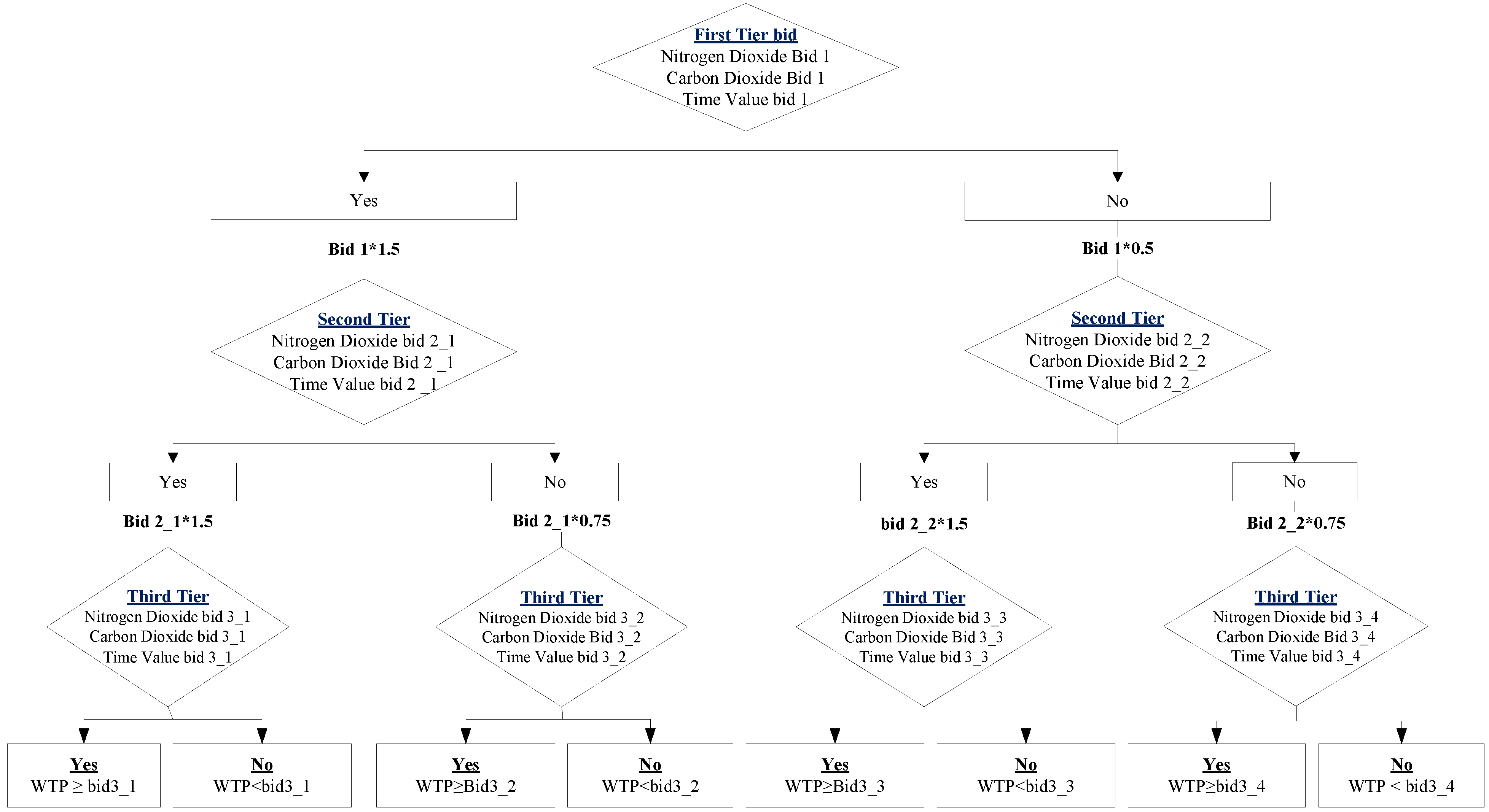
Figure 1. Triple-bound structure frame for air pollution WTP by parties to traffic accidents and time delay scenario for individuals affected by traffic accidents.

Figure 1. Triple-bound structure frame for air pollution WTP by parties to traffic accidents and time delay scenario for individuals affected by traffic accidents.

Subsequent price inquiries followed the triple-bound method (Figure 1), setting three tiers of bids, to more efficiently obtain interviewees’ real WTP. In the hypothetical market scenario section, as the survey follows skip logic with three-tier questions, there were eight possible answers: (1) Yes-Yes-Yes; (2) Yes-Yes-No; (3) Yes-No-Yes; (4) Yes-No-No; (5) No-Yes-Yes; (6) No-Yes-No; (7) No-No-Yes; and (8) No-No-No. In the eighth answer scenario, the interviewee indicates no to all three questions, meaning that he/she is not willing to pay the suggested bid on the third tier, and so the next step is to ask if the interviewee’s real WTP is $NT0.

3.2. Data Analysis

3.2.1. Socio-Economic Characteristics

Table 2 shows the interviewees’ socioeconomic characteristics. The majority of the interviewees in all three levels were male, accounting for 59.5%, 52.5% and 54.6%, respectively, whereas females accounted for fewer than 50% of the interviewees. The majority of the interviewees were 31 to 40 years of age, which accounted for 32.7%, 35.2% and 33.1% of the interviewees; the next-most-represented age groups were 21 to 31 and 41 to 50 years of age. With respect to educational levels, the highest percentage of interviewees had college or junior college degrees—58.9%, 59.0% and 58.6% in each respective category—followed by interviewees holding high school diplomas or master’s degrees. Occupation-wise, the service industry was the most represented among the interviewees, comprising 28.9%, 34.0% and 31.9% of the groups, followed by the commercial and industrial sectors. With respect to average personal monthly income, a plurality of interviewees earned $NT25,001–40,000—29.1%, 37.0% and 30.5%—followed by interviewees with incomes of less than $NT25,000 and $NT 40,001 to 60,000. With respect to average monthly household income, families with $NT40,001 to 60,000 represented the majority of interviewees—23.2%, 21.1% and 23.8% of each respective level—but families with incomes of $NT25,001 to 40,000, $NT60,00 to 80,000 or $NT100,001 to 150,000 were also represented in significant number. With respect to family size (including the interviewees), most of the families represented had either two or four family members, represented at 28.7% and 29.2% in the light scenario, 35.6% and 31.1% in the moderate scenario and 37.1% and 30.5% in the severe scenario.

Table 2. Socioeconomic characteristics analysis.

Item		Light		Moderate		Severe
		Sample Number	(%)	Sample Number	(%)	Sample Number	(%)
Gender	Male	180	(59.6)	159	(52.5)	165	(54.6)
	Female	122	(40.4)	144	(47.5)	137	(45.4)
Age	Under 20	14	(4.7)	16	(5.3)	17	(5.6)
	21–30	76	(25.2)	79	(26.1)	87	(28.8)
	31–40	99	(32.7)	107	(35.2)	100	(33.1)
	41–50	61	(20.2)	65	(21.5)	54	(17.9)
	51–60	40	(13.2)	28	(9.2)	28	(9.3)
	61 and above	12	(4.0)	8	(2.7)	16	(5.3)
Education Level	Elementary school, Junior high school	16	(5.3)	18	(5.9)	18	(5.9)
	(Vocational) high school	66	(21.9)	89	(29.4)	73	(24.2)
	College/Junior college	178	(58.9)	179	(59.0)	177	(58.6)
	Master’s/Doctoral degree	42	(13.9)	17	(5.7)	32	(10.6)
Occupation	Unemployed/Job-searching/Retired	15	(5.0)	10	(3.3)	24	(7.9)
	Homemaker	27	(8.9)	23	(7.6)	30	(9.9)
	Military, public or teaching	33	(10.9)	21	(6.9)	20	(6.6)
	Agricultural, forestry, fishery or animal husbandry	3	(1.0)	3	(1.0)	5	(1.7)
	Industry	43	(14.2)	49	(16.2)	52	(17.2)
	Commerce	73	(24.2)	63	(20.8)	45	(14.9)
	Service	87	(28.9)	103	(34.0)	96	(31.9)
	Students	17	(5.6)	20	(6.6)	19	(6.3)
	Others	4	(1.3)	11	(3.6)	11	(3.6)
Average Personal Monthly Income	25,000 and below	78	(25.8)	74	(26.4)	88	(29.2)
	25,001–40,000	88	(29.1)	112	(37.0)	92	(30.5)
	40,001–60,000	77	(25.5)	65	(21.5)	73	(24.2)
	60,001–80,000	29	(9.6)	34	(11.2)	24	(7.9)
	80,001–100,000	13	(4.3)	4	(1.3)	7	(2.2)
	100,001 and above	12	(3.9)	8	(2.6)	18	(6.0)
Average Household Monthly Income	25,000 and below	25	(8.3)	24	(8.0)	26	(8.6)
	25,001–40,000	44	(14.6)	62	(20.5)	46	(15.2)
	40,001–60,000	70	(23.2)	64	(21.1)	72	(23.8)
	60,001–80,000	46	(15.2)	56	(18.5)	45	(14.9)
	80,001–100,000	34	(11.3)	24	(7.9)	31	(10.3)
	100,001–150,000	40	(13.2)	35	(11.6)	42	(13.9)
	150,001–200,000	16	(5.3)	15	(5.0)	20	(6.6)
	200,001 and above	26	(8.6)	15	(5.0)	19	(6.3)
Family Size	1 person	47	(15.6)	31	(10.2)	39	(12.9)
	2 people	87	(28.7)	108	(35.6)	112	(37.1)
	3 people	80	(26.5)	70	(23.1)	59	(19.5)
	4 people and above	88	(29.2)	94	(31.1)	92	(30.5)
Total Sample Number		302		303		302

Note: There are two missing values (0.7%) for educational level in the severe scenario. There are five and six missing values in the light and moderate scenarios, respectively, for Personal Monthly Income; there are one, eight and one missing values in the light, moderate and severe scenarios, respectively, for Average Household Income.

Table 2. Socioeconomic characteristics analysis.

Item		Light		Moderate		Severe
		Sample Number	(%)	Sample Number	(%)	Sample Number	(%)
Gender	Male	180	(59.6)	159	(52.5)	165	(54.6)
	Female	122	(40.4)	144	(47.5)	137	(45.4)
Age	Under 20	14	(4.7)	16	(5.3)	17	(5.6)
	21–30	76	(25.2)	79	(26.1)	87	(28.8)
	31–40	99	(32.7)	107	(35.2)	100	(33.1)
	41–50	61	(20.2)	65	(21.5)	54	(17.9)
	51–60	40	(13.2)	28	(9.2)	28	(9.3)
	61 and above	12	(4.0)	8	(2.7)	16	(5.3)
Education Level	Elementary school, Junior high school	16	(5.3)	18	(5.9)	18	(5.9)
	(Vocational) high school	66	(21.9)	89	(29.4)	73	(24.2)
	College/Junior college	178	(58.9)	179	(59.0)	177	(58.6)
	Master’s/Doctoral degree	42	(13.9)	17	(5.7)	32	(10.6)
Occupation	Unemployed/Job-searching/Retired	15	(5.0)	10	(3.3)	24	(7.9)
	Homemaker	27	(8.9)	23	(7.6)	30	(9.9)
	Military, public or teaching	33	(10.9)	21	(6.9)	20	(6.6)
	Agricultural, forestry, fishery or animal husbandry	3	(1.0)	3	(1.0)	5	(1.7)
	Industry	43	(14.2)	49	(16.2)	52	(17.2)
	Commerce	73	(24.2)	63	(20.8)	45	(14.9)
	Service	87	(28.9)	103	(34.0)	96	(31.9)
	Students	17	(5.6)	20	(6.6)	19	(6.3)
	Others	4	(1.3)	11	(3.6)	11	(3.6)
Average Personal Monthly Income	25,000 and below	78	(25.8)	74	(26.4)	88	(29.2)
	25,001–40,000	88	(29.1)	112	(37.0)	92	(30.5)
	40,001–60,000	77	(25.5)	65	(21.5)	73	(24.2)
	60,001–80,000	29	(9.6)	34	(11.2)	24	(7.9)
	80,001–100,000	13	(4.3)	4	(1.3)	7	(2.2)
	100,001 and above	12	(3.9)	8	(2.6)	18	(6.0)
Average Household Monthly Income	25,000 and below	25	(8.3)	24	(8.0)	26	(8.6)
	25,001–40,000	44	(14.6)	62	(20.5)	46	(15.2)
	40,001–60,000	70	(23.2)	64	(21.1)	72	(23.8)
	60,001–80,000	46	(15.2)	56	(18.5)	45	(14.9)
	80,001–100,000	34	(11.3)	24	(7.9)	31	(10.3)
	100,001–150,000	40	(13.2)	35	(11.6)	42	(13.9)
	150,001–200,000	16	(5.3)	15	(5.0)	20	(6.6)
	200,001 and above	26	(8.6)	15	(5.0)	19	(6.3)
Family Size	1 person	47	(15.6)	31	(10.2)	39	(12.9)
	2 people	87	(28.7)	108	(35.6)	112	(37.1)
	3 people	80	(26.5)	70	(23.1)	59	(19.5)
	4 people and above	88	(29.2)	94	(31.1)	92	(30.5)
Total Sample Number		302		303		302

Note: There are two missing values (0.7%) for educational level in the severe scenario. There are five and six missing values in the light and moderate scenarios, respectively, for Personal Monthly Income; there are one, eight and one missing values in the light, moderate and severe scenarios, respectively, for Average Household Income.

Table 3 shows the interviewees’ travel characteristics. Their trip purposes were mostly tourism and leisure, with shares of 49.7%, 60.4% and 55.0%, respectively, followed by visiting families and friends and business trips. The majority of highway travel time was between 120 and 180 min, with shares of 26.8%, 25.4% and 29.5%; the remaining travel times are equally distributed. Travelling time on local roads was mostly less than 30 min, with shares of 36.5%, 47.8% and 35.8%, respectively; travel times of 120 min and above were the least common. Upwards of 80% of respondents’ travel was not time-sensitive; the likely reason for this result is that the study was conducted at highway rest areas, and most individuals who stopped at those rest areas were not pressed for time. With respect to traveller identity, most of the interviewees were drivers—62.6%, 54.5% and 57.6%, respectively. In addition, based on the location of the highway interchange that interviewees chose to enter/exit, we were able to further estimate highway travel distance. The distance is divided into three categories: short distances of fewer than 100 km; medium distances of between 100 and 200 km; and long distances of 300 km and above. Long distances comprised the majority of trips, with percentages of 40.1%, 41.2% and 37.1%, respectively.

Table 3. Travel characteristics analysis.

Item		Light		Moderate		Severe
		Sample Number	(%)	Sample Number	(%)	Sample Number	(%)
Trip Purpose	Work commute	30	(9.9)	24	(7.8)	19	(6.3)
	School commute	11	(3.6)	8	(2.6)	7	(2.3)
	Business	52	(17.2)	35	(11.6)	44	(14.6)
	Tourism/Leisure	150	(49.7)	183	(60.4)	166	(55.0)
	Visiting familiesand friends	51	(17.0)	45	(14.9)	58	(19.2)
	Other	8	(2.6)	8	(2.7)	8	(2.6)
Highway Travel Time	<60 min	55	(18.2)	49	(16.1)	42	(13.9)
	>=60 min, <120 min	45	(14.9)	59	(19.5)	48	(15.9)
	>=120 min, <180 min	81	(26.8)	77	(25.4)	89	(29.5)
	>=180 min, <240 min	60	(19.9)	55	(18.2)	61	(20.2)
	>=240 min	61	(20.2)	63	(20.8)	62	(20.5)
Local Road Travel Time	<30 min	110	(36.5)	145	(47.8)	108	(35.8)
	>=30 min, <60 min	94	(31.1)	97	(32.0)	104	(34.4)
	>=60 min, <120 min	71	(23.5)	39	(12.9)	50	(16.6)
	>=120 min	27	(8.9)	22	(7.3)	40	(13.2)
Traveller Identity	Driver	189	(62.6)	165	(54.5)	174	(57.6)
	Passenger	113	(37.4)	138	(45.5)	128	(42.4)
Highway Travel Distance	Short distance (<100 km)	91	(30.1)	85	(28.1)	89	(29.5)
	Medium distance (>=100, <300 km)	90	(29.8)	93	(30.7)	101	(33.4)
	Long distance (>=300 km)	121	(40.1)	125	(41.2)	112	(37.1)
Total Sample Number		302		303		302

Table 3. Travel characteristics analysis.

Item		Light		Moderate		Severe
		Sample Number	(%)	Sample Number	(%)	Sample Number	(%)
Trip Purpose	Work commute	30	(9.9)	24	(7.8)	19	(6.3)
	School commute	11	(3.6)	8	(2.6)	7	(2.3)
	Business	52	(17.2)	35	(11.6)	44	(14.6)
	Tourism/Leisure	150	(49.7)	183	(60.4)	166	(55.0)
	Visiting familiesand friends	51	(17.0)	45	(14.9)	58	(19.2)
	Other	8	(2.6)	8	(2.7)	8	(2.6)
Highway Travel Time	<60 min	55	(18.2)	49	(16.1)	42	(13.9)
	>=60 min, <120 min	45	(14.9)	59	(19.5)	48	(15.9)
	>=120 min, <180 min	81	(26.8)	77	(25.4)	89	(29.5)
	>=180 min, <240 min	60	(19.9)	55	(18.2)	61	(20.2)
	>=240 min	61	(20.2)	63	(20.8)	62	(20.5)
Local Road Travel Time	<30 min	110	(36.5)	145	(47.8)	108	(35.8)
	>=30 min, <60 min	94	(31.1)	97	(32.0)	104	(34.4)
	>=60 min, <120 min	71	(23.5)	39	(12.9)	50	(16.6)
	>=120 min	27	(8.9)	22	(7.3)	40	(13.2)
Traveller Identity	Driver	189	(62.6)	165	(54.5)	174	(57.6)
	Passenger	113	(37.4)	138	(45.5)	128	(42.4)
Highway Travel Distance	Short distance (<100 km)	91	(30.1)	85	(28.1)	89	(29.5)
	Medium distance (>=100, <300 km)	90	(29.8)	93	(30.7)	101	(33.4)
	Long distance (>=300 km)	121	(40.1)	125	(41.2)	112	(37.1)
Total Sample Number		302		303		302

Table 4 shows the interviewees’ physical health and participation in environmental activities. The survey listed eight popular environmental activities in Taiwan and asked interviewees about their willingness to participate in those activities. For example, bicycle parade, environmental protection parade, environmental protection lecture, beach or mountain cleaning activities, tree planting activities, trash off the ground, environmental protection competitions and Earth Day. From the table, we can see that in the three levels, 24.2%, 25.3% and 19.5% of the interviewees did not want to participate in environmental activities; 24.5%, 21.5% and 27.2% of the interviewees indicated a desire to participate in two environmental activities; and numerous interviewees indicated a desire to participate in either one or three environmental activities. Subsequently, interviewees were asked whether they had illnesses related air pollution such as eye irritation, respiratory diseases or cardiopulmonary diseases. From the table, we can see that interviewees were most likely to report respiratory diseases, with shares of 10.9%, 6.9% and 9.6%, respectively, with the next-largest group of interviewees reporting eye irritation, with shares of 4.0%, 4.3% and 3.3%.

Table 4. Analysis of physical health and participation in environmental activities.

Item		Light		Moderate		Severe
		Sample Number	(%)	Sample Number	(%)	Sample Number	(%)
Eye Irritation	No	290	(96.0)	290	(95.7)	292	(96.7)
	Yes	12	(4.0)	13	(4.3)	10	(3.3)
Respiratory Diseases	No	269	(89.1)	282	(93.1)	273	(90.4)
	Yes	33	(10.9)	21	(6.9)	29	(9.6)
Cardiopulmonary Diseases	No	297	(98.3)	295	(97.4)	301	(99.7)
	Yes	5	(1.7)	8	(2.6)	1	(0.3)
	No	73	(24.2)	77	(25.3)	59	(19.5)
Acceptable Number of Environmental Activities	1	59	(19.5)	57	(18.8)	56	(18.5)
	2	74	(24.5)	65	(21.5)	82	(27.2)
	3	49	(16.2)	50	(16.5)	60	(19.9)
	4	22	(7.3)	36	(11.9)	27	(8.9)
	5	15	(5.0)	10	(3.3)	9	(3.0)
	6	3	(1.0)	4	(1.3)	3	(1.0)
	7	3	(1.0)	2	(0.7)	1	(0.3)
	8	4	(1.3)	2	(0.7)	5	(1.7)
Total Sample Number		302		303		302

Table 4. Analysis of physical health and participation in environmental activities.

Item		Light		Moderate		Severe
		Sample Number	(%)	Sample Number	(%)	Sample Number	(%)
Eye Irritation	No	290	(96.0)	290	(95.7)	292	(96.7)
	Yes	12	(4.0)	13	(4.3)	10	(3.3)
Respiratory Diseases	No	269	(89.1)	282	(93.1)	273	(90.4)
	Yes	33	(10.9)	21	(6.9)	29	(9.6)
Cardiopulmonary Diseases	No	297	(98.3)	295	(97.4)	301	(99.7)
	Yes	5	(1.7)	8	(2.6)	1	(0.3)
	No	73	(24.2)	77	(25.3)	59	(19.5)
Acceptable Number of Environmental Activities	1	59	(19.5)	57	(18.8)	56	(18.5)
	2	74	(24.5)	65	(21.5)	82	(27.2)
	3	49	(16.2)	50	(16.5)	60	(19.9)
	4	22	(7.3)	36	(11.9)	27	(8.9)
	5	15	(5.0)	10	(3.3)	9	(3.0)
	6	3	(1.0)	4	(1.3)	3	(1.0)
	7	3	(1.0)	2	(0.7)	1	(0.3)
	8	4	(1.3)	2	(0.7)	5	(1.7)
Total Sample Number		302		303		302

3.2.2. Analysis of the Interviewees’ WTP

Table 5 shows WTP for nitrogen dioxide. The survey’s starting points were $NT10,000, $NT35,000 and $NT100,000 for light, moderate and severe levels, respectively. The majority of interviewees reporting a WTP of NT$0 represent 34.1%, 37.3% and 34.1% at each level. The reason for this may be due to Taiwan’s failure to enforce such measures; thus, most interviewees were not willing to pay the amounts listed in the survey.

Table 5. Analysis of WTP for nitrogen dioxide.

Light			Moderate			Severe
Price	Sample Number	(%)	WTP	Sample Number	(%)	WTP	Sample Number	(%)
WTP ≥ 22,500	10	(3.3)	WTP ≥ 80,000	4	(1.3)	WTP ≥ 250,000	7	(2.3)
WTP < 22,500	33	(10.9)	WTP < 80,000	11	(3.6)	WTP < 250,000	19	(6.3)
WTP ≥ 12,000	12	(4.0)	WTP ≥ 40,000	18	(5.9)	WTP ≥ 120,000	16	(5.3)
WTP < 12,000	35	(11.6)	WTP < 40,000	35	(11.6)	WTP < 120,000	23	(7.6)
WTP ≥ 7500	9	(3.0)	WTP ≥ 30,000	10	(3.3)	WTP ≥ 70,000	10	(3.3)
WTP < 7500	35	(11.6)	WTP < 30,000	12	(4.0)	WTP < 70,000	34	(11.3)
WTP ≥ 3500	34	(11.3)	WTP ≥ 10,000	61	(20.1)	WTP ≥ 35,000	45	(14.9)
WTP < 3500	31	(10.2)	WTP < 10,000	39	(12.9)	WTP < 35,000	45	(14.9)
WTP = 0	103	(34.1)	WTP = 0	113	(37.3)	WTP = 0	103	(34.1)
Sample Number	302		Sample Number	303		Sample Number	302

Table 5. Analysis of WTP for nitrogen dioxide.

Light			Moderate			Severe
Price	Sample Number	(%)	WTP	Sample Number	(%)	WTP	Sample Number	(%)
WTP ≥ 22,500	10	(3.3)	WTP ≥ 80,000	4	(1.3)	WTP ≥ 250,000	7	(2.3)
WTP < 22,500	33	(10.9)	WTP < 80,000	11	(3.6)	WTP < 250,000	19	(6.3)
WTP ≥ 12,000	12	(4.0)	WTP ≥ 40,000	18	(5.9)	WTP ≥ 120,000	16	(5.3)
WTP < 12,000	35	(11.6)	WTP < 40,000	35	(11.6)	WTP < 120,000	23	(7.6)
WTP ≥ 7500	9	(3.0)	WTP ≥ 30,000	10	(3.3)	WTP ≥ 70,000	10	(3.3)
WTP < 7500	35	(11.6)	WTP < 30,000	12	(4.0)	WTP < 70,000	34	(11.3)
WTP ≥ 3500	34	(11.3)	WTP ≥ 10,000	61	(20.1)	WTP ≥ 35,000	45	(14.9)
WTP < 3500	31	(10.2)	WTP < 10,000	39	(12.9)	WTP < 35,000	45	(14.9)
WTP = 0	103	(34.1)	WTP = 0	113	(37.3)	WTP = 0	103	(34.1)
Sample Number	302		Sample Number	303		Sample Number	302

Table 6 analyses WTP for carbon dioxide. The starting points of the survey were $NT1000, $NT2500 and $NT8000 for the light, moderate and severe levels, respectively. The majority WTP was NT$0, which were 31.1%, 34.3% and 35.1% at each level.

Table 6. Analysis of WTP for carbon dioxide.

Light			Moderate			Severe
Price	Sample Number	(%)	WTP	Sample Number	(%)	WTP	Sample Number	(%)
WTP ≥ 2500	46	(15.3)	WTP ≥ 6000	23	(7.6)	WTP ≥ 18,000	21	(7.0)
WTP < 2500	42	(13.7)	WTP < 6000	29	(9.6)	WTP < 18,000	31	(10.3)
WTP ≥ 1200	18	(6.0)	WTP ≥ 3000	24	(7.9)	WTP ≥ 9,000	26	(8.6)
WTP < 1200	50	(16.6)	WTP < 3000	41	(13.5)	WTP < 9,000	34	(11.3)
WTP ≥ 750	7	(2.3)	WTP ≥ 2000	7	(2.3)	WTP ≥ 6,000	11	(3.6)
WTP < 750	19	(6.3)	WTP < 2000	13	(4.3)	WTP < 6,000	22	(7.3)
WTP ≥ 350	21	(7.0)	WTP ≥ 1000	47	(15.5)	WTP ≥ 3,000	27	(8.9)
WTP < 350	5	(1.7)	WTP < 1000	15	(5.0)	WTP < 3,000	24	(7.9)
WTP = 0	94	(31.1)	WTP = 0	104	(34.3)	WTP = 0	106	(35.1)
Sample Number	302		Sample Number	303		Sample Number	302

Table 6. Analysis of WTP for carbon dioxide.

Light			Moderate			Severe
Price	Sample Number	(%)	WTP	Sample Number	(%)	WTP	Sample Number	(%)
WTP ≥ 2500	46	(15.3)	WTP ≥ 6000	23	(7.6)	WTP ≥ 18,000	21	(7.0)
WTP < 2500	42	(13.7)	WTP < 6000	29	(9.6)	WTP < 18,000	31	(10.3)
WTP ≥ 1200	18	(6.0)	WTP ≥ 3000	24	(7.9)	WTP ≥ 9,000	26	(8.6)
WTP < 1200	50	(16.6)	WTP < 3000	41	(13.5)	WTP < 9,000	34	(11.3)
WTP ≥ 750	7	(2.3)	WTP ≥ 2000	7	(2.3)	WTP ≥ 6,000	11	(3.6)
WTP < 750	19	(6.3)	WTP < 2000	13	(4.3)	WTP < 6,000	22	(7.3)
WTP ≥ 350	21	(7.0)	WTP ≥ 1000	47	(15.5)	WTP ≥ 3,000	27	(8.9)
WTP < 350	5	(1.7)	WTP < 1000	15	(5.0)	WTP < 3,000	24	(7.9)
WTP = 0	94	(31.1)	WTP = 0	104	(34.3)	WTP = 0	106	(35.1)
Sample Number	302		Sample Number	303		Sample Number	302

Table 7 shows WTP for time delays. The survey’s starting point for time delays caused by light, moderate and severe traffic accidents were $NT100, $NT300 and $NT500, respectively. The majority WTP was also $NT0, with shares of 31.5%, 32.7% and 26.2%.

Table 7. Analysis of WTP for time delays.

Light			Moderate			Severe
Price	Sample Number	(%)	WTP	Sample Number	(%)	WTP	Sample Number	(%)
WTP ≥ 250	52	(17.2)	WTP ≥ 700	42	(13.9)	WTP ≥ 1200	31	(13.3)
WTP < 250	74	(24.5)	WTP < 700	44	(14.5)	WTP < 1200	55	(18.2)
WTP ≥ 125	17	(5.6)	WTP ≥ 350	34	(11.2)	WTP ≥ 600	29	(9.6)
WTP < 125	39	(12.9)	WTP < 350	35	(11.6)	WTP < 600	59	(19.5)
WTP ≥ 75	3	(1.0)	WTP ≥ 250	10	(3.3)	WTP ≥ 350	6	(2.0)
WTP < 75	5	(1.6)	WTP<250	14	(4.6)	WTP < 350	17	(5.6)
WTP ≥ 35	12	(4.0)	WTP ≥ 100	14	(4.6)	WTP ≥ 150	16	(5.3)
WTP < 35	5	(1.7)	WTP < 100	11	(3.6)	WTP < 150	10	(3.3)
WTP = 0	95	(31.5)	WTP = 0	99	(32.7)	WTP = 0	79	(26.2)
Sample Number	302		Sample Number	303		Sample Number	302

Table 7. Analysis of WTP for time delays.

Light			Moderate			Severe
Price	Sample Number	(%)	WTP	Sample Number	(%)	WTP	Sample Number	(%)
WTP ≥ 250	52	(17.2)	WTP ≥ 700	42	(13.9)	WTP ≥ 1200	31	(13.3)
WTP < 250	74	(24.5)	WTP < 700	44	(14.5)	WTP < 1200	55	(18.2)
WTP ≥ 125	17	(5.6)	WTP ≥ 350	34	(11.2)	WTP ≥ 600	29	(9.6)
WTP < 125	39	(12.9)	WTP < 350	35	(11.6)	WTP < 600	59	(19.5)
WTP ≥ 75	3	(1.0)	WTP ≥ 250	10	(3.3)	WTP ≥ 350	6	(2.0)
WTP < 75	5	(1.6)	WTP<250	14	(4.6)	WTP < 350	17	(5.6)
WTP ≥ 35	12	(4.0)	WTP ≥ 100	14	(4.6)	WTP ≥ 150	16	(5.3)
WTP < 35	5	(1.7)	WTP < 100	11	(3.6)	WTP < 150	10	(3.3)
WTP = 0	95	(31.5)	WTP = 0	99	(32.7)	WTP = 0	79	(26.2)
Sample Number	302		Sample Number	303		Sample Number	302

4. Estimation Results

4.1. Variable Descriptions

Different variables were evaluated in the model; only those variables with significant estimation results are listed and discussed herein. From Table 8, we see that the dependent variables are WTP for nitrogen dioxide, carbon dioxide and time delays, and that the WTP range is as follows: $NT0–250,000 for nitrogen dioxide, $NT0–100,000 for carbon dioxide and $NT0–12,000 for time delays. The independent variables in this model estimation are dummy variables. In the hypothetical scenario for nitrogen dioxide, based on a priori knowledge, variables with a significant positive effect in the estimation model are as follows: “age 41 years and above”; “Education level of college or above”; “Willing to participate in two or more environmental activities”; “Eye irritation and respiratory diseases”; “Regular employee and average personal monthly income of NT$25,000 or more”; “Married and has a family size of two or fewer”; and “Willing to participate in environmental activities and average monthly household income is NT$60,000 or more”.

In the case of carbon dioxide, variables that have a significant positive effect in the estimation model include “Age between 31and 60”; “Education level of college or above”; “Personal monthly income of NT$40,000 and above”; “Eye irritation and respiratory diseases”; “Willing to participate in one or two environmental activities”; “Age 51 years or above and willing to participate in environmental activities ”, and “Education level of college or above and average monthly household income is NT$60,000 or above”.

For time delays, variables that have a significant positive effect in this estimation model include “managerial rank”; “work/school commute”; “travelling as the driver”; “two hours or more highway travel time”; “long travel distance (≥100 km) on this trip”; “short travel distance (<100 km) on this trip”. The model estimation was conducted based on the variables in the table.

4.2. Results

This section includes the WTP estimation model results for nitrogen dioxide, carbon dioxide and time delays, which are discussed separately. From the model estimation, we can see that the spike values shown in the estimation results are the WTP of the sample data. The WTP estimation results for nitrogen dioxide are shown in Table 9. The estimation result shows that WTP per metric ton is NT$11,502 for the light level, NT$9004 for the moderate level and NT$8862 for the severe level. Based on the unit cost of varied serious level, while the air pollution is more serious and the total value of WTP of interviewees increases, the relative average cost (NT$/metric ton) decreases.

Table 8. Variable definitions.

Dependent Variable
Variable	Range
1. Nitrogen dioxide scenarios	Light: 0–100,000
	Moderate: 0–100,000
	Severe: 0–250,000
2. Carbon dioxide scenarios	Light: 0–50,000
	Moderate: 0–100,000
	Severe: 0–100,000
3. Time delay scenarios	Light: 0–5,000
	Moderate: 0–10,000
	Severe: 0–12,000
Independent Variable
Variable	Range	Expectation
Age 41 years and above	1, otherwise 0	+1
Age between 31and 60	1, otherwise 0	+2
Education level of college or above	1, otherwise 0	+1, 2
Personal monthly income of NT$40,000 and above	1, otherwise 0	+2
Willing to participate in two or more environmental activities	1, otherwise 0	+1
Eye irritation and respiratory diseases	1, otherwise 0	+1,2
Willing to participate in one or two environmental activities	1, otherwise 0	+2
Managerial rank	1, otherwise 0	+3
Work/school commute	1, otherwise 0	+3
Travelling as the driver	1, otherwise 0	+3
Travel time of two hours or more for this trip	1, otherwise 0	+3
Long travel distance (≥100 km) for this travel	1, otherwise 0	+3
Short travel distance (<100 km) for this travel	1, otherwise 0	+3
Interactive Variable
Regular employee and average personal monthly income of NT$25,000 or more	1, otherwise 0	+1
Married and has a family size of two or fewer	1, otherwise 0	+1
Willing to participate in environmental activities and average monthly household income is NT$60,000 or more	1, otherwise 0	+1
Age 51 years or above and willing to participate in environmental activities	1, otherwise 0	+2
Education level of college or above and average monthly household income is NT$60,000 or above	1, otherwise 0	+2

Notes: 1 indicates nitrogen dioxide scenarios; 2 indicates carbon dioxide scenarios; 3 indicates time delay scenarios.

Table 8. Variable definitions.

Dependent Variable
Variable	Range
1. Nitrogen dioxide scenarios	Light: 0–100,000
	Moderate: 0–100,000
	Severe: 0–250,000
2. Carbon dioxide scenarios	Light: 0–50,000
	Moderate: 0–100,000
	Severe: 0–100,000
3. Time delay scenarios	Light: 0–5,000
	Moderate: 0–10,000
	Severe: 0–12,000
Independent Variable
Variable	Range	Expectation
Age 41 years and above	1, otherwise 0	+1
Age between 31and 60	1, otherwise 0	+2
Education level of college or above	1, otherwise 0	+1, 2
Personal monthly income of NT$40,000 and above	1, otherwise 0	+2
Willing to participate in two or more environmental activities	1, otherwise 0	+1
Eye irritation and respiratory diseases	1, otherwise 0	+1,2
Willing to participate in one or two environmental activities	1, otherwise 0	+2
Managerial rank	1, otherwise 0	+3
Work/school commute	1, otherwise 0	+3
Travelling as the driver	1, otherwise 0	+3
Travel time of two hours or more for this trip	1, otherwise 0	+3
Long travel distance (≥100 km) for this travel	1, otherwise 0	+3
Short travel distance (<100 km) for this travel	1, otherwise 0	+3
Interactive Variable
Regular employee and average personal monthly income of NT$25,000 or more	1, otherwise 0	+1
Married and has a family size of two or fewer	1, otherwise 0	+1
Willing to participate in environmental activities and average monthly household income is NT$60,000 or more	1, otherwise 0	+1
Age 51 years or above and willing to participate in environmental activities	1, otherwise 0	+2
Education level of college or above and average monthly household income is NT$60,000 or above	1, otherwise 0	+2

Notes: 1 indicates nitrogen dioxide scenarios; 2 indicates carbon dioxide scenarios; 3 indicates time delay scenarios.

In the estimation model, the negative coefficient of bid shows that for those interviewees who are willing to participate in the nitrogen dioxide pollution offset, the higher the bid, the more interviewees are reluctant to pay. This result is consistent with the expectations of the present study. From the table, we see that the variables that have significant positive effects include “age 40 years or above”, “college/junior college degree or above”, “eye irritation or respiratory diseases”, and “willing to participate in two or more environmental activities”. Interviewees who are 40 years of age or older and who have a college/junior college degree or above have greater WTP. This is likely because these groups of travellers have better comprehension and judgment and therefore are more willing to pay for pollution emissions caused by traffic accidents for which they are responsible.

Table 9. Model estimation result of WTP for nitrogen dioxide.

Variable	Light		Moderate		Severe
	Coefficient	t-value	Coefficient	t-value	Coefficient	t-value
Constant	−0.03	(−0.20)	0.12	(0.83)	−0.14	(−0.94)
Bid	−0.83	(−6.46 **)	−0.36	(−7.31 **)	−0.14	(−9.51 **)
Age 41 years or above	0.60	(2.90 **)	0.37	(1.92 *)	─	─
College/junior college degree or above	0.51	(2.65 **)	─	─	0.91	(5.14 **)
Eye irritation or respiratory diseases	0.82	(1.99 **)	─	─	2.00	(2.05 **)
Willing to participate in two or more environmental activities	0.67	(2.19 **)	─	─	─	─
Married with family size of two or fewer	─	─	0.79	(1.92 *)	─	─
Willing to participate in environmental activities and average monthly household income is NT$60,000 or above	─	─	0.73	(1.71 *)	0.81	(1.91 *)
Regular employee and average personal monthly income of NT$25,000 or more	─	─	0.36	(2.27 **)	─	─
WTP (NT$/metric ton)	11,502	(5.57 **)	9,004	(6.29 **)	8,862	(7.40 **)
Spike value	0.38	(9.29 **)	0.38	(10.05 **)	0.32	(9.93 **)
Wald statistic (p-value)	9.29		285.33		405.96
Log likelihood function	−306.68		−324.82		−318.53
Sample number	302		303		302

Notes: * indicates significant level of 0.1; ** indicates significant level of 0.05.

Table 9. Model estimation result of WTP for nitrogen dioxide.

Variable	Light		Moderate		Severe
	Coefficient	t-value	Coefficient	t-value	Coefficient	t-value
Constant	−0.03	(−0.20)	0.12	(0.83)	−0.14	(−0.94)
Bid	−0.83	(−6.46 **)	−0.36	(−7.31 **)	−0.14	(−9.51 **)
Age 41 years or above	0.60	(2.90 **)	0.37	(1.92 *)	─	─
College/junior college degree or above	0.51	(2.65 **)	─	─	0.91	(5.14 **)
Eye irritation or respiratory diseases	0.82	(1.99 **)	─	─	2.00	(2.05 **)
Willing to participate in two or more environmental activities	0.67	(2.19 **)	─	─	─	─
Married with family size of two or fewer	─	─	0.79	(1.92 *)	─	─
Willing to participate in environmental activities and average monthly household income is NT$60,000 or above	─	─	0.73	(1.71 *)	0.81	(1.91 *)
Regular employee and average personal monthly income of NT$25,000 or more	─	─	0.36	(2.27 **)	─	─
WTP (NT$/metric ton)	11,502	(5.57 **)	9,004	(6.29 **)	8,862	(7.40 **)
Spike value	0.38	(9.29 **)	0.38	(10.05 **)	0.32	(9.93 **)
Wald statistic (p-value)	9.29		285.33		405.96
Log likelihood function	−306.68		−324.82		−318.53
Sample number	302		303		302

Notes: * indicates significant level of 0.1; ** indicates significant level of 0.05.

Additionally, it is reasonable to assume that interviewees who are willing to participate in two or more environmental activities are more environmentally conscious and thus are more willing to pay a penalty for nitrogen dioxide emissions caused by traffic accidents. Furthermore, when these type of interviewees also have illnesses such as eye irritation or respiratory diseases, they are more likely to be sensitive to air pollution conditions than are interviewees who do not have such symptoms, in turn increasing the first group’s WTP. It is evident that the coefficient value 0.82 has the most significant effect in the model. The estimation result of this model is in accordance with the results shown in the study of Wang and Zhang [13], which indicate that household income/expense, respiratory diseases, education level, and opinions on air pollution and health-related issues are the significant variables that influence air quality improvement.

In moderate and severe levels, more interactive variables are included and are significant statistically. It shall be noted that compensation amounts rise as the pollution level rises. Therefore, interviewees with lower socioeconomic backgrounds may not be able to pay fees; interviewees must be environmentally conscious and also have a high income to be able to pay higher compensation. For example, the variables “Married and has a family size of two or fewer”, “Willing to participate in environmental activities and average monthly household income is NT$60,000 or above” and “Regular employee and has an average monthly income of NT$25,000 or above” have positive and significant effects at the moderate level of pollution caused by traffic accidents. We also assume that interviewees who are willing to participate in environmental activities feel obligated to pay higher amounts to compensate for nitrogen dioxide pollution for which he/she is responsible. However, when the pollution level is moderate or severe, we do not consider willingness to participate in environmental activities, interviewees must have an average household monthly income of NT$60,000 to demonstrate a higher WTP to compensate for nitrogen dioxide emissions caused by traffic accidents, meaning that only those interviewees whose families have superior economic well-being at a certain level can afford and are willing to pay compensation. In order to afford the pollution compensation fee, interviewees may have to be married and have fewer than two family members (without the economic burden of child support). Subsequently, compared to part-time workers, full-time employees have more secure employment, and only with an average monthly income of more than NT$25,000 can interviewees afford the fee, and thus have a higher WTP.

Table 10 shows the analysis of the WTP estimation results for carbon dioxide. The average WTP is NT$2693 in the light level, NT$1120 in the moderate level, and NT$1070 in the severe level. From the table, we can see that the significant positive effects in the light level belong to variables such as “personal monthly income of NT$40,000 or above”, “college/junior college degree or above”, “Age between 31 and 60 years” and “Willing to participate in two or two environmental activities”. This result is most likely because an average personal monthly income of NT$40,000 is almost equal the national average personal monthly income of approximately NT$44,798 (Accounting and Statistics, Executive Yuan, R.O.C., 2013) [10], and therefore, interviewees with this income level can afford the extra expense and are more willing to pay carbon dioxide compensation fees triggered by traffic accidents. The other three variables are similar to the explanations shown in the nitrogen dioxide estimation results: it is likely because these interviewees have higher comprehension and judgment abilities and pay more attention to the greenhouse effect caused by carbon dioxide emissions; in other words, they are environmentally conscious and therefore are more willing to pay for carbon dioxide caused by traffic accidents.

In terms of the moderate level, we can see that interviewees with eye irritation and respiratory diseases, “Age between 31 and 60 years” and “Willing to participate in two or two environmental activities” are more willing to pay compensation fees for carbon dioxide. The reasons are similar to the explanations mentioned earlier. Because a severe pollution level requires a higher compensation fee, only the variables of “eye irritation or respiratory diseases” and “Age 51 years or above and willing to participate in environmental activities” show a significant positive effect on WTP. Moreover, from the coefficient value of 0.79, we can see that this has the biggest impact on the model. Therefore, this group of interviewees should be the target audience for any future promotion of this policy. Finally, interviewees must be well-educated and also have a high income to be able to pay higher compensation. For example, the variable “Education level of college or above and average monthly household income is NT$60,000 or above” has positive and significant effects at the severe level of pollution caused by traffic accidents.

Table 10. Model estimation result of WTP for carbon dioxide.

Variable	Light		Moderate		Severe
	Coefficient	t-value	Coefficient	t-value	Coefficient	t-value
Constant	−0.08	(−0.40)	0.18	(1.18)	0.01	(0.09)
Bid	−0.53	(−4.85 **)	−0.29	(−7.02 **)	−0.12	(−8.42 **)
Age between 31 and 60	0.35	(1.92 *)	0.37	(2.33 **)	─	─
Education level of college or above	0.41	(2.01 **)	─	─	─	─
Personal monthly income of NT$40,000 or above	0.46	(1.99 **)	─	─	─	─
Eye irritation or respiratory diseases	─	─	1.11	(1.81 *)	0.72	(2.11 **)
Willing to participate in one or two environmental activities	0.37	(1.79*)	0.34	(1.94 *)	─	─
Age 51 years or above and willing to participate in environmental activities	─	─	─	─	0.79	(1.96 **)
Education level of college or above and average monthly household income is NT$60,000 or above	─	─	─	─	0.38	(1.74*)
WTP(NT$/metric ton)	2,693	(4.10 **)	1,120	(6.34 **)	1,070	(4.27 **)
Spike value	0.32	(5.22 **)	0.37	(7.40 **)	0.32	(4.32 **)
Wald statistic (p-value)	283.87		205.14		267.26
Log likelihood function	−331.58		−331.82		−316.22
Sample number	302		303		302

Notes: * indicates significant level of 0.1; ** indicates significant level of 0.05.

Table 10. Model estimation result of WTP for carbon dioxide.

Variable	Light		Moderate		Severe
	Coefficient	t-value	Coefficient	t-value	Coefficient	t-value
Constant	−0.08	(−0.40)	0.18	(1.18)	0.01	(0.09)
Bid	−0.53	(−4.85 **)	−0.29	(−7.02 **)	−0.12	(−8.42 **)
Age between 31 and 60	0.35	(1.92 *)	0.37	(2.33 **)	─	─
Education level of college or above	0.41	(2.01 **)	─	─	─	─
Personal monthly income of NT$40,000 or above	0.46	(1.99 **)	─	─	─	─
Eye irritation or respiratory diseases	─	─	1.11	(1.81 *)	0.72	(2.11 **)
Willing to participate in one or two environmental activities	0.37	(1.79*)	0.34	(1.94 *)	─	─
Age 51 years or above and willing to participate in environmental activities	─	─	─	─	0.79	(1.96 **)
Education level of college or above and average monthly household income is NT$60,000 or above	─	─	─	─	0.38	(1.74*)
WTP(NT$/metric ton)	2,693	(4.10 **)	1,120	(6.34 **)	1,070	(4.27 **)
Spike value	0.32	(5.22 **)	0.37	(7.40 **)	0.32	(4.32 **)
Wald statistic (p-value)	283.87		205.14		267.26
Log likelihood function	−331.58		−331.82		−316.22
Sample number	302		303		302

Notes: * indicates significant level of 0.1; ** indicates significant level of 0.05.

The WTP estimation results for time delays are shown in Table 11. From the table, we can see that WTP for one hour is NT$1315 for the light level, NT$1027 for the moderate level and NT$960 for the severe level. Overall, travellers identifying as drivers has a positive effect on WTP for time delays caused by traffic accidents at three levels. This is most likely because interviewees who are drivers had stronger and direct feelings about driving time and therefore were more willing to pay. In addition, work/school commute and short travelling distance also have positive effects only on the light level. The result of short travelling distance is possibly because travel time is comparatively short in short-distance travel, making a 10-minute delay represent a large proportion of the entire trip (32.2% approximately); therefore, short-distance travellers are willing to pay to avoid time delays.

Table 11. Model estimation results of WTP for time delays.

Item	Light		Moderate		Severe
	Coefficient	t-value	Coefficient	t-value	Coefficient	t-value
Constant	0.10	(0.62)	0.39	(2.37 **)	0.25	(1.72 *)
Bid	−5.37	(−6.95 **)	−2.11	(−6.82 **)	−1.25	(−14.24 **)
Traveller is driver	0.71	(3.61 **)	0.31	(1.73 *)	0.30	(1.65 *)
Work/school commute	0.39	(1.83 *)	─	─	─	─
Travel time of two hours or more for this trip	─	─	0.31	(1.69 *)	0.58	(2.64 **)
Medium highway travel distance for this trip (≥100 km, <300 km)	─	─	0.45	(1.96 **)	0.88	(3.71 **)
Short highway travel distance for this trip (<100 km)	0.77	(3.29 *)	─	─	─	─
Managerial rank	─	─	─	─	0.60	(1.75 *)
WTP (NT$/hour)	1315	(5.98 **)	1,027	(6.41 **)	960	(6.95 **)
Spike value	0.31	(5.98 **)	0.34	(8.02 **)	0.30	(5.94 **)
Wald statistic (p-value)	206.68		189.36		683.25
Log likelihood function	−342.71		−338.97		−343.92
Sample number	302		303		302

Note: * indicates significant level of 0.1; ** indicates significant level of 0.05.

Table 11. Model estimation results of WTP for time delays.

Item	Light		Moderate		Severe
	Coefficient	t-value	Coefficient	t-value	Coefficient	t-value
Constant	0.10	(0.62)	0.39	(2.37 **)	0.25	(1.72 *)
Bid	−5.37	(−6.95 **)	−2.11	(−6.82 **)	−1.25	(−14.24 **)
Traveller is driver	0.71	(3.61 **)	0.31	(1.73 *)	0.30	(1.65 *)
Work/school commute	0.39	(1.83 *)	─	─	─	─
Travel time of two hours or more for this trip	─	─	0.31	(1.69 *)	0.58	(2.64 **)
Medium highway travel distance for this trip (≥100 km, <300 km)	─	─	0.45	(1.96 **)	0.88	(3.71 **)
Short highway travel distance for this trip (<100 km)	0.77	(3.29 *)	─	─	─	─
Managerial rank	─	─	─	─	0.60	(1.75 *)
WTP (NT$/hour)	1315	(5.98 **)	1,027	(6.41 **)	960	(6.95 **)
Spike value	0.31	(5.98 **)	0.34	(8.02 **)	0.30	(5.94 **)
Wald statistic (p-value)	206.68		189.36		683.25
Log likelihood function	−342.71		−338.97		−343.92
Sample number	302		303		302

Note: * indicates significant level of 0.1; ** indicates significant level of 0.05.

In the moderate and severe levels, interviewees whose travel time was two hours or more were more willing to pay for time delays caused by traffic accidents, possibly trying to avoid longer travel times. Interviewees with medium travelling distance have a positive effect on WTP in the moderate and severe levels. Travelling time is naturally longer for medium-distance travellers, and therefore a 10-min delay in travelling time has relatively little impact. Therefore, medium-distance travellers only have a stronger WTP when time delays are more serious in moderate and severe levels, i.e., when time delays equal 30 or 60 min. Finally, in the severe level, interviewees at the managerial level have a stronger WTP to avoid time delays. This is likely because the value of these interviewees’ time is higher due to their professional rank; therefore, when faced with a long time delay, they are more willing to pay a higher amount to prevent the delay from happening.

Compared the WTP for time loss to other studies, the results show that Taiwanese value of time is close to the United States (as shown in Table 12).

Table 12. Comparisons of value of time.

Sources	Country	Value of Time (US$/hour)
Our study	Taiwan	32–43
Ghosh [40]	U.S.A.	20–57
Brownstone [41]	U.S.A.	23–43
Steimetz and Brownstone[42]	U.S.A.	46

Table 12. Comparisons of value of time.

Sources	Country	Value of Time (US$/hour)
Our study	Taiwan	32–43
Ghosh [40]	U.S.A.	20–57
Brownstone [41]	U.S.A.	23–43
Steimetz and Brownstone[42]	U.S.A.	46

5. Conclusions and Recommendations

This study adopted the TBDC method to estimate WTP. Interviewees’ WTPs were obtained using three tiers of price inquiry. The spike model was used to estimate the WTP for air pollution due to traffic accidents caused by the parties, along with the affected individuals’ WTP for time delays due to traffic accidents caused by them. This section proposes conclusions and recommendations based on this study’s research findings.

From the WTP estimation model of nitrogen dioxide and carbon dioxide, we can see that age, income, education level, willingness to participate in environmental activities and cross-variables such as average monthly income combined with willingness to participate in environmental activities affect the results of the model. In both models, as the severity of pollution and the compensation amount both rise, the interviewees’ WTP is influenced by more than a single socioeconomic characteristic; multiple characteristics such as high income or environmental consciousness are required for a positive effect on WTP. In the time delays model, variables such as occupational rank, trip purpose, traveller identity, travel time and travel distance have positive effects on WTP. Because the severity of traffic accidents differs, the level of air pollution and time loss differ significantly. The interviewees’ WTP also differs depending on the level of severity. In the case of nitrogen dioxide, the average WTP is NT$11,502 for the light level, NT$9004 for the moderate level and NT$8862 for the severe level. For carbon dioxide, the average WTP is NT$2693 for the light level, NT$1120 for the moderate level and NT$1070 for the severe level. With respect to time loss, the average WTP for an hour is NT$1315 for light congestion, $1027 for moderate congestion and $960 for severe congestion.

However, in Taiwan there is no standard method to measure air pollution caused by traffic accidents, and the severity (light, moderate or severe) of pollution was not included in the traffic accident database. With respect to time delays caused by traffic accidents, only the overview of traffic accidents (including estimated time delay and distance) gathered by the Taiwanese Police Radio Station was collected, and there were no complete traffic accident investigation records that could be utilised. Therefore, we suggest that in the future, traffic accident data should include factors such as the air pollution, processing time and amount of traffic congestion caused by traffic accidents. Only through determining the different types of pollution levels and time delays caused by traffic accidents can different compensation levels be calculated to provide a reference point for the external cost of traffic accidents.

We believe that individuals who cause traffic accidents should compensate for the impact of air pollution and time delays caused by those accidents, a position that is consistent with the polluter-pays principle—utilising the income of the polluter to compensate for air pollution and time loss. Although this measure has not been implemented, this study obtains WTP for air pollution by individuals who cause traffic accidents, which in turn provides a reference for relevant agencies to establish an applicable sanction standard. However, this study is the first attempt to study an air pollution and time loss compensation amount targeted at the parties or individuals in traffic accidents; therefore, the research area is confined to highway users. We recommend that future studies be expanded to local roads for the purpose of obtaining more complete research data.