Efficiency versus Equality: Comparing Design Options for Indirect Emissions Accounting in the Korean Emissions Trading Scheme

Abstract

The Korean emissions trading scheme (ETS) has one special characteristic that makes it different from other schemes, such as the EU ETS. While the other schemes consider only direct emissions from fossil fuels, the Korean ETS also regulates indirect emissions arising from the consumption of electricity. The problem of double counting arises under this setting, in which emissions from the power sector can be accounted for twice, when electricity is produced and consumed. This study aims to compare design options on indirect emissions accounting for the Korean ETS using a computable general equilibrium model. Four scenarios are generated for options accounting for direct and/or indirect emissions and are evaluated in terms of efficiency and equality. The result shows that the ETS operates most efficiently when only direct emissions are considered. However, the option that includes both direct and indirect emissions produces a competent result in terms of equality by spreading the economic burden of emissions reduction among industries. We conclude that this option can be an alternative to meet the key purposes of the Korean ETS.

1. Introduction

In 2011, Korea (South Korea) was the seventh biggest country emitter of greenhouse gases (GHG), emitting 697.7 Mt of carbon dioxide equivalent (CO₂e). From 1990 to 2011, Korea’s level of emissions has more than doubled [1]. To cope with the rapid growth rate of GHG emissions, the Korean government has pledged to the international community to reduce its GHG emissions by 30% by 2020 relative to the projected business-as-usual (BAU) level. A domestic emissions trading scheme (ETS) has been implemented from 2015 as a tool to achieve the reduction target [2,3].

However, the current design of the Korean ETS has some special characteristics compared to most existing ETSs. In particular, the Korean ETS regulates indirect emissions from the consumption of electricity, whereas the EU ETS considers only direct emissions. This structural difference of the Korean ETS can lead to double counting in emissions accounting since the activities of generating and consuming electricity require the simultaneous use of emissions allowances [2,4,5,6]. Nevertheless, the Korean government has pushed accounting for indirect emissions for the following reasons: (1) reducing the electricity intensity of the economy; (2) transferring the carbon price to the consumption side; and (3) equally spreading the burden of emissions abatement across industrial sectors.

This study aims to analyze and compare design options on indirect emissions accounting for the Korean ETS using a computable general equilibrium (CGE) model. CGE models have been used heavily to compare design options for ETSs, including the EU ETS [7,8,9,10,11] and Korean ETS [12,13]. However, there has been no attempt to simulate indirect emissions accounting, which is inherent in the design of the Korean ETS. In this study, four scenarios on design options on indirect emissions accounting are evaluated in terms of efficiency and equality using the CGE model. In addition, we considered the Renewable Portfolio Standards (RPS) for the electricity sector based on the Korean government’s initiatives.

Our study is significant in that it offers a quantitative analysis of macroeconomic and sectoral effects in response to different design options of the Korean ETS. The result shows that the ETS operates most efficiently when only direct emissions are considered. However, the scenario that includes both direct and indirect emissions provides a competent result in terms of equality by spreading the economic burden of emissions reduction among industries. Scenarios reveal some trade-off situations between efficiency and equality in achieving the carbon mitigation target. We expect that the simulation results based on the Korean economy can also give valuable information to the policy makers in East Asian countries and other countries with similar industrial landscapes.

The rest of this paper is structured as follows. Section 2 provides a brief overview of the Korean ETS, focusing on the background to implementing the scheme. Section 3 contains general descriptions of the CGE model used for the analyses. Section 4 explains the scenario settings. The main results are presented in Section 5. Lastly, the summary and concluding remarks are provided in Section 6.

2. Distinctive Features of the Korean ETS

GHG emissions can be classified into different scopes, based on the source of the emissions: Scope 1 emissions are direct emissions from activities owned or controlled by organizations that release emissions straight into the atmosphere. Examples of Scope 1 emissions include emissions from combustion in owned or controlled boilers and owned or controlled vehicles. Scope 2 emissions are associated with the consumption of purchased electricity, heat, steam and cooling. These are indirect emissions that are a consequence of an organization’s activities, but that occur at sources that organizations do not own or control. The most common type of Scope 2 emissions is electricity purchased for own consumption from the national grid [14,15,16,17,18].

The definition of GHG emissions by the Korean government includes both Scope 1 and Scope 2 emissions. According to the Framework Act on Low Carbon Green Growth, the term “emissions of greenhouse gases” encompasses “both direct emissions of greenhouse gases, which refers to emissions, discharges, or leaks of greenhouse gases generated as a consequence of human activities, and indirect emissions of greenhouse gases, which refers to discharges of greenhouse gases using electricity or heat (limited to emissions from a heat source generated with fuel or electricity) supplied by another person” [19]. Ultimately, the Korean ETS regulating domestic GHG emissions covers direct and indirect emissions simultaneously.

The ETSs adopted by major countries and regions (e.g., EU ETS) cover only Scope 1 emissions from fossil fuels burned on site. On the other hand, the Korean ETS regulates both Scopes 1 and 2 emissions simultaneously, which can lead to double counting of emissions, since such activities as generating and consuming electricity require the simultaneous use of emissions allowances. Despite this structural peculiarity, the Korean government has adopted the current ETS design for the following reasons.

First, the process of power sector privatization in Korea is not fully complete, and the price of electricity is still controlled heavily by the government. Immense political pressure would accompany any increase in the consumer price of electricity to reflect the cost of electricity generation properly. Under this situation, the price of electricity cannot be adjusted properly to reflect the additional cost from emissions by fossil fuel combustion in electricity generation when the ETS is implemented. Thus, the government is imposing a carbon price on electricity consumers by regulating indirect emissions to transfer the burden of emissions abatement partially to the consumption side [6].

In practice, the Korean ETS only regulates large emitters, such as power plants and manufacturing firms, rather than small emitters, such as households. Thus, from the perspective of political difficulties in policy implementation, imposing the carbon price on electricity use for the industrial sectors by the ETS (with indirect emission accounting) can be a relatively easy way compared to directly adding the carbon price on the retail price of electricity. Since increasing the retail electricity price will directly impact the household consumption and bring about instant opposition and political pressure, ETS regulating the large (direct and indirect) emitters will indirectly affect the household economy.

In terms of the pass through rate of CO₂ costs, the situation in Korea is very different from EU ETS. Empirical studies [7,9] estimating the pass through rates of CO₂ costs to power prices in EU countries [7] found that pass through rates range between 60% and 120% in EU countries under the assumption of perfect competition, while [9] showed that this rate is over 100% for The Netherlands, Belgium, Germany and France. In addition, [20] also found that cost pass through rates are close to 100% when the demand is inelastic, while this rate fell to around 80% with elastic demand. However, this pass through rate of the carbon costs can be near zero when the electricity price is regulated [21], which is similar to the Korean case.

Second, the Korean government stresses “equality” as one of the key principles in operating an ETS, which means that the economic burden of emissions abatement should not be concentrated to a few specific sectors (e.g., energy-intensive sectors, such as cement, iron, steel, chemicals and refining), but shared across industries and major companies. However, many of Korea’s very large companies, such as electronic manufacturers, have very little direct emissions and would not be included in the ETS if indirect emissions were not covered. In addition, some of the top 10 entities would be primarily indirect emitters using electricity as their main energy source. Thus, if the ETS were to regulate only direct emissions, many of the biggest and most promising companies in Korea would be free from the emissions abatement burden, and it would be difficult to meet the equality principle, as abatement costs would be focused on only a few energy-intensive industries [22]. This is particularly true when the price of electricity cannot be increased freely to reflect the carbon abatement cost. If the ETS only regulates the direct emissions along with a malfunctioning pricing system for electricity (without CO₂ cost pass through from the electricity sector), industries using electricity as their main energy sources will face less economic burden than industries using fossil fuels for their energy sources, leading to disparities among industries.

Third, with poor indigenous energy resources, Korea has to rely on imports to meet almost its entire energy demand. Saving electricity and decreasing the electricity dependency of the economy has become one of the top priority goals of Korea’s energy policy, since substantial amounts of imported primary energy are lost during generation, transmission and distribution of electricity. However, Korea has shown rapid rates of electrification, and the share of electricity in final energy consumption has grown by 5.7% annually, increasing from 10.8% in 1990 to 19.3% in 2012 [23]. When carbon costs are passed through to consumers appropriately, electricity consumers have incentives to reduce the electricity consumption [24,25]. However, the carbon price pass through mechanism of the competitive market does not work in the Korean ETS in the presence of market imperfection and government price regulation on the electricity sector [6]. Under this background, the Korean ETS covering indirect emissions has been implemented as a demand-side measure, since it makes consumers pay for the additional carbon price when they consume electricity [2,6].

Apart from the Korean ETS, other schemes exist that regulate indirect emissions. For example, the China regional level ETSs have been implemented in seven provinces as pilot schemes since 2013 [26,27,28]. The electricity sector in China is also heavily regulated by the government, and the carbon costs cannot be easily passed on to consumers, which may be a cause of market distortions [6,27,28]. Another important consideration for including indirect emissions is that in some provinces, indirect emissions (occurring by using electricity imported from other provinces) account for a significant share of total emissions [27]. Therefore, all of the regional level ETS pilots in China cover the indirect emissions. Under this scheme, indirect emissions from both electricity generation within the pilot region and imported electricity from outside pilot regions are covered in all of the pilot schemes [29]. In addition, the Japanese government has proposed the nationwide ETS, including the regulation of indirect emissions for electricity consumers, along with direct emissions for electricity producers. It is also understandable considering the electricity market in Japan, which is controlled by the government. This implies the lack of an appropriate pass through of carbon costs to the final electricity consumers [6,30,31]. The regional level ETS (in Tokyo) has also been implemented in Japan since 2010, which covers both indirect and direct CO₂ emissions from the use of energy [31]. However, until now, the Korean ETS is the only scheme applied nationwide among the ETSs that have already been implemented.

In summary, the main purpose of including indirect emissions within the Korean ETS is to incentivize electricity consumers (industries and households) to reduce electricity consumption, as the current price signal cannot be passed to electricity consumers. Hence, it can be understood that with inclusions of indirect emissions, the Korean government aims to decrease the electricity dependency under rapid electrification trends and the spread the burden of emissions reduction equally across sectors.

3. Model Description

3.1. Outline of the Model

The CGE model developed for analysis is a small open-economy model of the Korean economy. Labor and capital are considered as primary factors of production, which are employed together with energy and material inputs to produce domestic output. Nested, separable constant elasticity of substitution (CES) production functions are employed to represent the substitution possibilities among capital, labor, energy and material inputs (Figure 1).

Figure 1. Nested production structure of industries (except the electricity sector). CES, constant elasticity of substitution.

Figure 1. Nested production structure of industries (except the electricity sector). CES, constant elasticity of substitution.

The production of commodities is represented by the nested CES production functions, as shown in Figure 1. At the top level, a composite of intermediate material inputs (M) is traded off against a value added-energy composite (VAE) subject to CES. Value added-energy composite (VAE) is comprised of energy aggregate (E) and value-added composite. At the second level, a CES function captures the substitution possibilities between the energy aggregate (E) and a value-added composite (VA) of labor and capital. At the third level, capital and labor substitution possibilities within the value-added composite are described by a CES function, whereas different energy inputs (coal, gas, oil and electricity) enter the energy composite subject to CES. Values for substitution elasticities between production factors of each sector are adopted from [32] (Table 1).

Table 1. Key parameters in the model.

Parameter	Description	Value	Comments
${\text{σ}}_{VA}$	Elasticity of substitution between labor and capital	0.02~0.46	Varies by sector
${\text{σ}}_{VAE}$	Elasticity of substitution between energy and value added	0.00~0.60	Varies by sector
${\text{σ}}_M$	Elasticity of substitution among intermediate inputs	0.00~0.60	Varies by sector
${\text{σ}}_{VAEM}$	Elasticity of substitution between intermediates and the aggregate of value added and energy inputs	0.00~1.17	Varies by sector
${\text{σ}}_{OG}$	Elasticity of substitution between oil and gas energy inputs	0.5	All sectors
${\text{σ}}_{OGC}$	Elasticity of substitution between the aggregate of oil and gas and coal energy inputs	0.5	All sectors
${\text{σ}}_{ELE}$	Elasticity of substitution among different energy inputs (coal, gas, oil and electricity)	0.5	All sectors
${\text{σ}}_{DM}$	Elasticity of substitution between domestic goods and imports	4	All sectors

Table 1. Key parameters in the model.

Parameter	Description	Value	Comments
${\text{σ}}_{VA}$	Elasticity of substitution between labor and capital	0.02~0.46	Varies by sector
${\text{σ}}_{VAE}$	Elasticity of substitution between energy and value added	0.00~0.60	Varies by sector
${\text{σ}}_M$	Elasticity of substitution among intermediate inputs	0.00~0.60	Varies by sector
${\text{σ}}_{VAEM}$	Elasticity of substitution between intermediates and the aggregate of value added and energy inputs	0.00~1.17	Varies by sector
${\text{σ}}_{OG}$	Elasticity of substitution between oil and gas energy inputs	0.5	All sectors
${\text{σ}}_{OGC}$	Elasticity of substitution between the aggregate of oil and gas and coal energy inputs	0.5	All sectors
${\text{σ}}_{ELE}$	Elasticity of substitution among different energy inputs (coal, gas, oil and electricity)	0.5	All sectors
${\text{σ}}_{DM}$	Elasticity of substitution between domestic goods and imports	4	All sectors

Final consumption demand is determined by the representative household, which maximizes welfare subject to its budget constraint consisting of net factor income and tax revenues. The consumption demand of the representative agent is comprised of energy and non-energy consumption goods. In the model, it is assumed that the investment and provision of public goods and services are given exogenously. In addition, Armington’s approach [33] is adopted, which distinguishes between domestic and foreign goods. All goods used in intermediate and final demand correspond to a CES composite that combines the domestically-produced goods and imported goods.

The model uses energy and economy datasets of Korea, such as the social accounting matrix from the input-output table, energy balance data [34] and GHG emissions data [35], setting the year 2010 as the base year. The production sector comprises 21 sectors consisting of eight energy sectors and 13 non-energy sectors (Table 2), with energy commodities divided into coal, crude oil, coke, natural gas, manufactured gas, naphtha, fuel oil and electricity. In Figure 1, “oil” consists of naphtha (NAP) and fuel oil (FOL), “gas” consists of natural gas (NGA) and manufactured gas (GAS) and “coal” consists of coal (COL) and coke (CKC).

Table 2. Sector classifications of the model.

Sector	Descriptions
Energy Sectors
COA	Anthracite, bituminous coal, coal briquettes
CRU	Crude oil (imported)
NGA	Natural gas (imported)
GAS	Manufactured gas
CKC	Coke and other coal products
NAP	Naphtha and miscellaneous refinery products
FOL	Fuel oil (except for naphtha) and liquefied petroleum gas
ELE	Electricity and heat
Non-Energy Sectors
AFF	Agriculture, forestry and fishing
TNL	Textile and leather
MIN	Mining and quarrying
FOO	Food and tobacco
PPP	Paper, pulp and print
CRP	Petroleum, chemical and rubber
NMP	Nonmetallic minerals products
ORE	Iron and steel
NFM	Nonferrous metal products
FAM	Fabricated metal products
TRN	Transportation
SER	Commercial and public services
ETC	Other non-specified sectors

Table 2. Sector classifications of the model.

Sector	Descriptions
Energy Sectors
COA	Anthracite, bituminous coal, coal briquettes
CRU	Crude oil (imported)
NGA	Natural gas (imported)
GAS	Manufactured gas
CKC	Coke and other coal products
NAP	Naphtha and miscellaneous refinery products
FOL	Fuel oil (except for naphtha) and liquefied petroleum gas
ELE	Electricity and heat
Non-Energy Sectors
AFF	Agriculture, forestry and fishing
TNL	Textile and leather
MIN	Mining and quarrying
FOO	Food and tobacco
PPP	Paper, pulp and print
CRP	Petroleum, chemical and rubber
NMP	Nonmetallic minerals products
ORE	Iron and steel
NFM	Nonferrous metal products
FAM	Fabricated metal products
TRN	Transportation
SER	Commercial and public services
ETC	Other non-specified sectors

3.2. Modeling the Electricity Sector

The production structure of the electricity sector is different from other industries, as represented in Figure 2. Electricity is generated from different technologies using various resources, such as coal, gas, oil, nuclear and renewables. Capital input for each generation technology is treated as the fixed factor, specifically belonging to each technology. This fixed factor reflects the capacity restrictions of each generation technology [36,37,38,39] and is combined with other inputs consisting of intermediate composites and labor inputs to produce electricity. The substitution elasticities of ${\text{σ}}_{tr}^X$ within the CES production structure are calibrated consistently with exogenously-given supply elasticities of each generation technology [40,41]. Supply elasticity can represent how flexibly each technology can change its generation capacity in response to demand. For example, we set lower values of supply elasticities for generation technologies that are constructed under the government plan over the long term, such as nuclear power plants, and relatively higher values for those that could be built in short periods and operated flexibly, such as gas power plants and renewable energy power plants.

Figure 2. Nested production structure of the electricity sector.

Figure 2. Nested production structure of the electricity sector.

3.3. Business-As-Usual Scenario

The model is built and calibrated based on the energy and economic situation in Korea in 2010. However, since this analysis aims to observe the impact of achieving the emissions reduction target of 2020, the BAU scenario up to 2020 is generated by expanding the base-year economy incorporating various projection data. Projection data contain forecast figures for long-term economic growth (gross domestic product (GDP) forecasts), energy price forecasts, energy demand by source, GHG emissions by source and generation mix forecasts. We use the forecast values for GDP growth (Table 3) and crude oil prices from the U.S. Energy Information Administration (EIA) [42,43], and assume fossil fuel prices are linked to changes of crude oil prices (Table 4). In addition, to set the BAU scenarios, the projections for energy demand by sector are taken from research by the Korea Energy Economics Institute (KEEI) [44] and generation mix forecasts from the EIA [42]. In addition, we calculate the GHG emissions from each sector by energy sources based on the energy balance data from the KEEI [34,35,45].

Table 3. GDP projections for business-as-usual (2010 = 1).

Year	2010	2011	2012	2013	2014	2015	2016	2017	2018	2019	2020
GDP Level	1.00	1.04	1.06	1.10	1.15	1.21	1.26	1.31	1.37	1.42	1.47

Table 3. GDP projections for business-as-usual (2010 = 1).

Year	2010	2011	2012	2013	2014	2015	2016	2017	2018	2019	2020
GDP Level	1.00	1.04	1.06	1.10	1.15	1.21	1.26	1.31	1.37	1.42	1.47

Table 4. Crude oil price projections for business-as-usual (2010 = 1).

Year	2010	2011	2012	2013	2014	2015	2016	2017	2018	2019	2020
Crude Oil Price Level	1.00	1.37	1.34	1.19	1.19	1.18	1.19	1.22	1.25	1.27	1.30

Table 4. Crude oil price projections for business-as-usual (2010 = 1).

Year	2010	2011	2012	2013	2014	2015	2016	2017	2018	2019	2020
Crude Oil Price Level	1.00	1.37	1.34	1.19	1.19	1.18	1.19	1.22	1.25	1.27	1.30

3.4. Modelling Direct and Indirect Emissions

In the production structure represented in Figure 1, fossil fuel inputs, such as coal, coke, gas and fuel oil, are combined with “carbon credits” or emissions allowances by a Leontief function. This means that to use fossil fuel in the production process, emissions allowances are required in proportion to the amount of fossil fuel and its carbon content, which represents the burden from direct emissions of the production side of each sector. As depicted in Figure 2, to generate electricity, the electricity sector also requires carbon credits, which are associated with the amount of fossil fuel inputs.

In addition, it is important to reflect indirect emissions accounting of the Korean ETS in the model. Therefore, each industrial sector requires allowances for indirect emissions when consuming electricity. This allowance is represented in Figure 1 as an “indirect carbon credit.” The level of indirect emissions per unit consumption of electricity, which is proportional to the CO₂ emissions factor of electricity, can be changed when the fuel mix of the power sector is changed. Since electricity cannot be stored, all electricity generated is consumed in the economy, and thus, we assume that the level of direct emissions from generating electricity and the level of indirect emissions from consuming electricity should be equalized. Hence, the indirect emissions factor for the consumption of electricity is calculated through an iteration process within the model to equalize direct emissions from generating electricity (“carbon credit” in Figure 2) and indirect emissions from consuming electricity (“indirect carbon credit” in Figure 1). The initial value is set as the level of entire emissions from the electricity sector divided by the amount of output in the electricity sector.

Additionally, it is also important to check the price elasticity of electricity demand, before going through analyzing each scenario’s effect. Lower demand elasticity for electricity would increase the level of cost pass through [9,20,21], making the inclusion of the indirect emissions within the ETS have very little effect. Thus, the value for demand elasticity of electricity has been calculated by running the BAU scenario with an exogenous output tax increase/decrease by 1% on the electricity sector. From the simulations, the absolute value of demand elasticity is estimated to be around 0.49. It is found that the demand elasticity of electricity drawn from our model shows similar or higher levels compared to other estimation results from various countries [46,47,48,49].

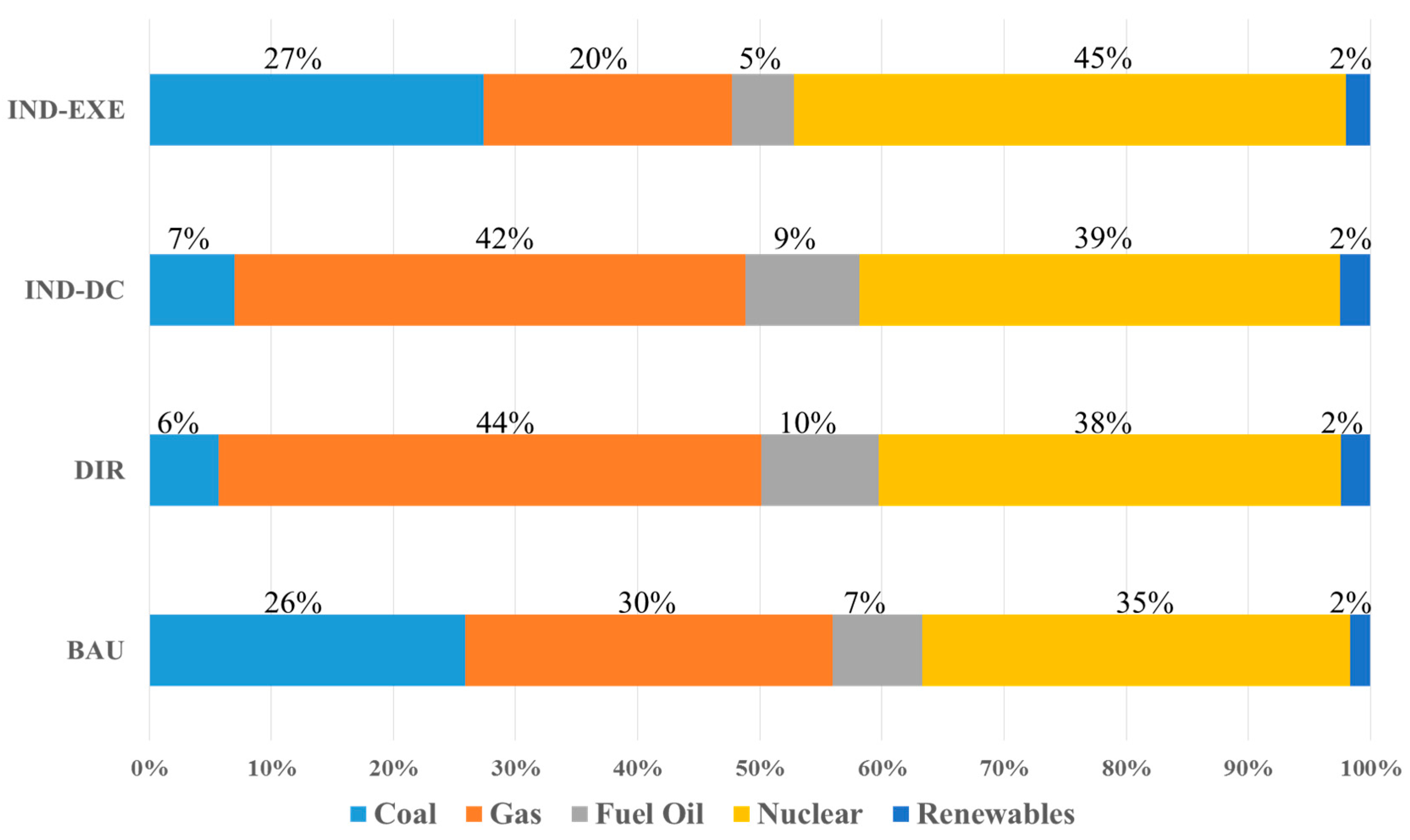
4. Scenario Settings

This study analyzes and compares the design options of the Korean ETS using a CGE model. Our model considers only CO₂ emissions from fossil fuel combustion to avoid the complexity of analysis and owing to data availability. It is assumed that the entire economy is covered by the ETS. The emissions allowances, which eventually set the level of emissions and emissions reduction of the economy, are first owned by the government and, then, are auctioned to firms requiring carbon credits in producing outputs.

The scenarios are generated on the following options: (1) regulation of only direct emissions within the ETS as a reference scenario; (2) regulation of both direct and indirect emissions within the ETS with double counting; (3) regulation of both direct and indirect emissions within the ETS, along with the exemption of the electricity sector from direct emissions coverage, in order to avoid double counting on emissions allowances; and (4) setting the RPS for the electricity sector within each scenario.

4.1. Direct Emission Scenario

The “direct emissions” (DIR) scenario is assumed to implement an ETS that considers only direct emissions. Under the DIR scenario, the reduction target (emissions constraint) of the Korean economy is equivalent to the total amounts of emissions allowances. The total credit amount is given under the assumption that Korea achieves a target of 30% reduction from the BAU level of emissions in 2020. All other scenarios generated in this research are also modeled on the assumption of achieving the same reduction target in 2020 to guarantee the comparability of the results among scenarios.

4.2. Indirect Emissions Double Counting Scenario

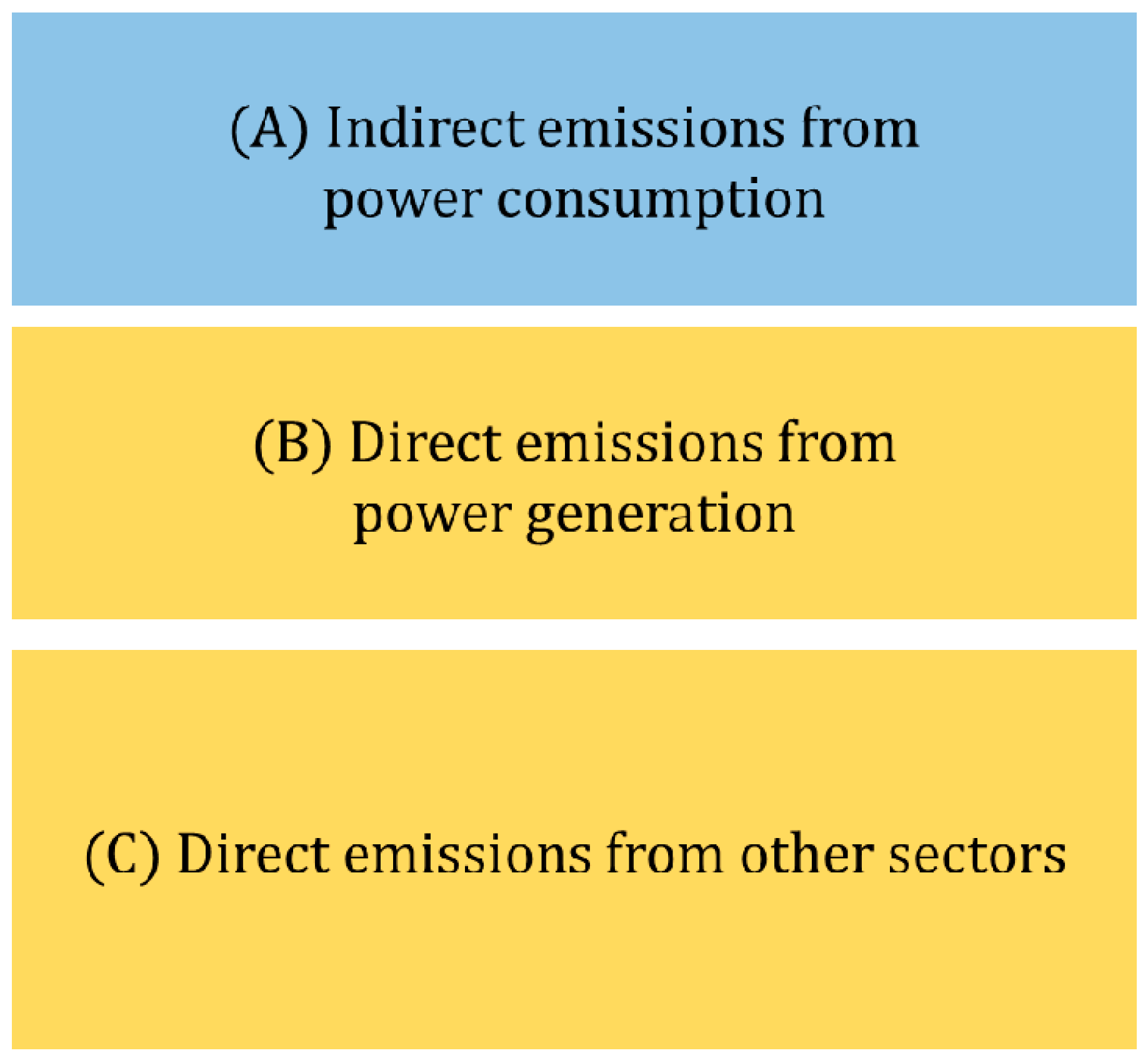
The “indirect emissions double counting” (IND-DC) scenario includes indirect emissions within the ETS. Under this option, double counting occurs in emissions accounting, since generating and consuming electricity require the simultaneous use of emissions allowances. In this case, when the total amount of allowances is the same as the DIR scenario, the actual abatement level will be higher than the reduction target. This is because when double counting occurs, the demand for credits from electricity consumption increases. Thus, if a scheme also covers indirect emissions, it needs to supply more allowances than the total level of direct emissions. This issue is illustrated in Figure 3. Under the DIR scenario, the amount of allowances needed to achieve the reduction target is {(B) + (C)}, which represents direct emissions from the economy. However, under the IND-DC scenario, the amount of allowances needed is {(A) + (B) + (C)} because of double counting.

Figure 3. Amount of emissions allowances for each scenario.

Figure 3. Amount of emissions allowances for each scenario.

Our model shows that under the IND-DC scenario, which fixes the allowances supply equal to the level of the DIR scenario, the actual abatement level in 2020 shows a 41.5% reduction from the BAU level, which is far higher than the reduction target of 30%. Therefore, in order to keep the reduction level at 30% from the BAU by 2020, it is necessary to increase the amount of allowances supplied. Our model calculates that the amount of allowances needed under the IND-DC scenario is estimated to be 25.4% higher than the allowance level for the DIR case. Thus, the value of a carbon credit, measured as a right to emit one ton of CO₂e, could be lower than that of other schemes, since more allowances are needed for the same level of emissions from the economy. Hence, the IND-DC scenario can cause credibility problems, especially when implementing linkages with other international carbon markets.

4.3. Exemption of Electricity Sector within the Direct Emissions Coverage Scenario

Another design option for “including indirect emissions” within the ETS is “exempting direct emissions from the electricity sector” (IND-EXE). In this case, emissions from the electricity sector are accounted for only as indirect emissions from electricity consumption. Under this policy alternative, CO₂ emissions arising from generating electricity are transferred entirely to electricity consumers via indirect emissions. This structural design of the ETS can avoid issues of double counting allowances and does not cause credibility problems of carbon credits. In Figure 3, the amount of allowances for this scenario is set as {(A) + (C)}, which is the same as the DIR scenario, since we assumed that the amount of (A) is equal to the amount of (B) in this model.

However, the power sector, which usually has large abatement potential, can entirely avoid burdens for emissions reduction in this case. As a result, the burden from the electricity sector is shifted to other sectors with less abatement potential (i.e., electricity consumers), causing an increased burden for overall industry in the Korean economy.

4.4. Renewable Portfolio Standards Scenario

We consider here Korea’s renewable energy expansion policy, namely, the Renewable Portfolio Standards (RPS), with policy design options for the ETS based on scenario settings as discussed previously: DIR/R, IND-DC/R and IND-EXE/R. “R scenario” is the abbreviation for implementation of “renewable energy expansion policy”. To expand renewable power production and reduce GHG emissions in Korea, the RPS has been implemented since 2012. RPS is a quantity-based regulation for the electricity sector, in which the government sets quotas to ensure that a certain market share of electricity generation comes from renewable energy sources [50]. Under this scenario, the share of renewable energies in total power production is assumed to increase up to 6% in 2020. An overview of those scenarios is represented briefly in Table 5.

Table 5. Overview of scenario setting. BAU, business-as-usual; DIR, direct emissions; IND-DC, indirect emissions double counting; IND-EXE, exempting direct emissions from the electricity sector; RPS, Renewable Portfolio Standards; ETS, emissions trading scheme.

Scenarios	Description
BAU	⋅ No obligations for CO2 reduction
	⋅ Base year economy is expanded using various projections to 2020
DIR	⋅ 30% CO2 reduction from the BAU in 2020
	⋅ Only covers direct emissions within the ETS
IND-DC	⋅ 30% CO2 reduction from the BAU in 2020
	⋅ Covers both direct and indirect emissions
	⋅ Emission from the electricity sector is double counted
	⋅ The level of allowance supply is 125.4% of the DIR case
IND-EXE	⋅ 30% CO2 reduction from the BAU in 2020
	⋅ Covers both direct and indirect emissions, exempting the electricity sector from the direct emissions coverage
RPS (DIR/R, IND-DC/R, IND-EXE/R)	⋅ Additionally considers the RPS on the electricity sector upon the DIR, IND-DC and IND-EXE scenarios
	⋅ The share of renewable energies in power production is set as 6% in 2020

Table 5. Overview of scenario setting. BAU, business-as-usual; DIR, direct emissions; IND-DC, indirect emissions double counting; IND-EXE, exempting direct emissions from the electricity sector; RPS, Renewable Portfolio Standards; ETS, emissions trading scheme.

Scenarios	Description
BAU	⋅ No obligations for CO2 reduction
	⋅ Base year economy is expanded using various projections to 2020
DIR	⋅ 30% CO2 reduction from the BAU in 2020
	⋅ Only covers direct emissions within the ETS
IND-DC	⋅ 30% CO2 reduction from the BAU in 2020
	⋅ Covers both direct and indirect emissions
	⋅ Emission from the electricity sector is double counted
	⋅ The level of allowance supply is 125.4% of the DIR case
IND-EXE	⋅ 30% CO2 reduction from the BAU in 2020
	⋅ Covers both direct and indirect emissions, exempting the electricity sector from the direct emissions coverage
RPS (DIR/R, IND-DC/R, IND-EXE/R)	⋅ Additionally considers the RPS on the electricity sector upon the DIR, IND-DC and IND-EXE scenarios
	⋅ The share of renewable energies in power production is set as 6% in 2020

5. Results and Implications

5.1. Macroeconomic Effects

In this subsection, we illustrate the main results representing the economic impacts of different design options. It is shown that scenario DIR is the most cost-effective way to achieve the reduction target in 2020 when analyzing the macroeconomic effects in terms of GDP and consumption level, as represented in Table 6.

Table 6 reveals that the losses of GDP and consumption level under the IND-DC and IND-EXE scenarios are greater than those under the DIR case. There is a minor difference when comparing the level of GDP losses between the DIR and IND-DC scenarios (DIR: −0.62% vs. IND-DC: −0.71%). However, the IND-EXE case reveals significant losses of −2.59% from the BAU GDP level. In the case of IND-EXE, the electricity sector, which has large potential for abatement, is exempted from regulations for direct emissions, and burdens for emissions reduction are transferred to other sectors, resulting in increased economic losses to the economy. The high level of GDP loss for IND-EXE implies that the scenario has little practical importance.

Table 6. Macroeconomic effects under different scenarios.

Indicator	Scenario
	DIR		IND-DC		IND-EXE
	DIR	DIR/R	IND-DC	IND-DC/R	IND-EXE	IND-EXE/R
GDP level (% changes relative to BAU)	−0.62	−0.65	−0.71	−0.74	−2.59	−2.36
Consumption level (% changes relative to BAU)	−0.61	−0.68	−0.68	−0.74	−2.43	−2.26
Carbon price (unit: thousand KRW a)	47.9	47.5	47.3	46.8	188.6	174.8

^a 1 U.S. dollar = 1131.5 Korean won (KRW) in October 2015.

Table 6. Macroeconomic effects under different scenarios.

Indicator	Scenario
	DIR		IND-DC		IND-EXE
	DIR	DIR/R	IND-DC	IND-DC/R	IND-EXE	IND-EXE/R
GDP level (% changes relative to BAU)	−0.62	−0.65	−0.71	−0.74	−2.59	−2.36
Consumption level (% changes relative to BAU)	−0.61	−0.68	−0.68	−0.74	−2.43	−2.26
Carbon price (unit: thousand KRW a)	47.9	47.5	47.3	46.8	188.6	174.8

^a 1 U.S. dollar = 1131.5 Korean won (KRW) in October 2015.

On the other hand, when looking into the carbon price (emissions allowance price), the IND-DC scenario shows a lower price level than the DIR scenario (DIR: 47.9 thousand Korean won (KRW); vs. IND-DC: 47.3 thousand KRW). However, the value of a carbon credit, measured as the right to emit one ton of CO₂e, for the IND-DC scenario is different from the DIR scenario, since the amount of allowances supplied under the IND-DC scenario is 125.4% of the level of the DIR scenario for the same reduction target. Therefore, under the IND-DC scenario, one unit of carbon credit can permit emissions of only 100/125.4 tons of CO₂e. When the value of the credit is adjusted to guarantee the right to emit one ton of CO₂e as in the DIR scenario, the price of the credit for the IND-DC scenario should be adjusted to 59.1 thousand KRW (which is 125.4% of 47.3 thousand KRW), which is higher than the level of the DIR scenario (47.9 thousand KRW), which is quite natural considering the higher GDP loss of the IND-DC scenario (−0.71%) than the DIR scenario (−0.62%).

Furthermore, looking at scenarios that consider implementation of the RPS on the electricity sector, we can see that the GDP decrease of the DIR scenario is −0.62%, while that of the DIR/R scenario is −0.65% compared to the BAU level. This is because imposition of additional RPS on the electricity sector in the presence of the ETS can lead to excess costs of producing electricity [51,52,53]. This results in an increased electricity price and reduced output from the electricity sector, and hence, the overall sectors’ production activities shrink with less consumption of electricity. As a result, losses of GDP and consumption level under the DIR/R and IND-DC/R scenarios are greater than those under the DIR and IND-DC scenarios, as represented in Table 6. However, different aspects appear when comparing the level of GDP losses between the IND-EXE/R and IND-EXE scenarios (IND-EXE: −2.59% vs. IND-EXE/R: −2.36%). Under the IND-EXE scenario, CO₂ emissions arising from electricity generation are transferred entirely to electricity consumers as a form of indirect emissions. As a result, the electricity sector has no obligations to reduce emissions. However, the implementation of the RPS (IND-EXE/R) in the absence of obligations for emissions reduction can place a burden on the electricity sector to avoid using carbon-intensive fuels and technologies. Under this scheme, sectors other than electricity face relatively less burden in consuming electricity when introducing RPS on the electricity sector as a form of regulation.

5.2. Sectoral Effects

5.2.1. Sectoral Effects in Terms of Production Activities

This subsection describes how changes in production levels of the main sectors appear in different scenarios. Figure 4 depicts the changes of production levels in the main sectors relative to the BAU level.

Figure 4. Changes of the production level in the main sectors relative to the business-as-usual (BAU) level.

Figure 4. Changes of the production level in the main sectors relative to the business-as-usual (BAU) level.

Figure 4 shows that the production level of major industries and energy-intensive industries in Korea, such as the petrochemical, steel, non-metallic products and fabricated metal products sectors, shrank in all scenarios (Figure 4). When comparing the absolute level of output losses by scenario type, Figure 4 reveals that the production losses are comparatively smaller in the DIR scenario, while the IND-EXE scenario shows significant losses in production activities.

However, when we compare the IND-EXE and IND-EXE/R scenarios, Figure 4 shows that industries face fewer losses in output levels when introducing the RPS in the presence of the ETS (IND-EXE/R) compared to cases that adopt the ETS only (IND-EXE). For example, Figure 4 shows that the production losses faced by the steel industry in the IND-EXE scenario (−36.1% from the BAU level) is reduced in the IND-EXE/R scenario (−34.7% from the BAU level). This is because the expansion of renewable electricity generation by imposing the RPS depresses the carbon price, resulting in benefits to carbon-intensive sectors [54,55,56].

5.2.2. Sectoral Effects in Terms of Burden Sharing and Equality

The Korean ETS pays special attention to spreading the burden of emissions reduction equally across sectors. To analyze how the burden for abatement is spread across all industries, the concept of a national average index (NAI) is adopted. The NAI is commonly used to measure the industrial diversities of regional economies [57,58,59]. For example, [57] attempts to calculate the NAI to summarize information about changes in the distribution of economic activity (e.g., employment) in a single indicator and uses the percentage of employment in each industry by regional level to calculate the NAI.

In Equation (1), when $P_i$ is the market share of industry i in a region of interest and $M_i$ is the market share of industry i of a nation, the value of the NAI will be close to zero when the regional industrial structure is similar to the industrial structure of the nation and will have larger positive value when the regional economy is specialized in some specific industry and, hence, is very different from the national industrial structure.

$$\text{National Average Index}={{\displaystyle \sum }}_i\left[\raisebox{1ex}{${\left(P_i-M_i\right)}^2$}\!\left/ \!\raisebox{-1ex}{$M_i$}\right.\right]$$

(1)

However, we apply the NAI to establish how the industrial structure has changed through emissions abatement from the BAU for each scenario. In our analysis, $P_i$ is the market share (%) of each sector for each scenario, and $M_i$ is the market share (%) of each sector in the BAU scenario. If the burden of abatement is focused on some specific industry, then the industrial structure changes substantially from the BAU situation, and the NAI comparing the scenario with the BAU situation might have a higher positive value, while a lower value for the NAI can be expected when the burden is distributed equally and the industrial structure has not changed much. Table 7 shows the calculated NAI values for each scenario.

Table 7. Calculated national average index (NAI) under different scenarios.

Indicator	Scenario
	DIR	DIR/R	IND-DC	IND-DC/R	IND-EXE	IND-EXE/R
NA Index	0.115	0.105	0.108	0.101	0.633	0.573

Table 7. Calculated national average index (NAI) under different scenarios.

Indicator	Scenario
	DIR	DIR/R	IND-DC	IND-DC/R	IND-EXE	IND-EXE/R
NA Index	0.115	0.105	0.108	0.101	0.633	0.573

As represented in Table 7, the IND-DC scenario shows a smaller NAI value than the DIR and IND-EXE scenarios, with 0.108 representing relatively equalized burdens of abatement costs across sectors. Therefore, the structural design of the Korean ETS with double counting of allowances (IND-DC) is understood to operate in a way that enhances sharing of the burden among industries. Furthermore, imposition of the RPS has greater effects on achieving the equality principle for all scenarios. The imposition of the RPS and subsequent decrease in the carbon price decreases the concentration of the burden on energy-intensive sectors.

5.3. Effects on the Electricity Sector

As discussed in Section 2, with rapid rates of electrification and increasing electricity intensity, the Korean government has implemented the ETS, including indirect emissions, as a measure of demand-side management to save electricity use. Therefore, it is meaningful to observe key indicators related to the electricity sector (Table 8). In the IND-DC and IND-EXE scenarios, the price of electricity differs between the consumer and producer sides, since additional carbon costs are reflected in the consumer price. The IND-DC scenario shows greater decreases in the power generation level (−11% from the BAU level) compared to the DIR scenario (−7.4% from the BAU level). This can be accounted for by the rise in the consumer price of electricity.

The ETS that covers indirect emissions also requires emissions allowances when electricity is consumed. Therefore, the consumer price of electricity increases much more with the inclusion of the carbon price under the ETS covering direct and indirect emissions compared to the case that regulates only direct emissions. Accordingly, the consumer price of the IND-DC scenario increases by 30.7% compared to the BAU scenario, while that of the DIR scenario increases by 15.8% compared to the BAU level. The higher consumer price of electricity causes a much greater fall in the demand for electricity, resulting in greater decreases of electricity production. In this context, owing to the highest consumer price of electricity of all scenarios (108% increase from the BAU level), the IND-EXE scenario shows the greatest electricity generation decline (−22.3% from the BAU level) among all scenarios. Furthermore, as shown in Table 8, the electricity intensity of the IND-DC scenario is much lower (−10.3% from the BAU level) than the DIR scenario (−6.8% from the BAU level). The result shows that the ETS regulating indirect emissions (IND-DC) works better in reducing the electricity intensity of the economy compared to ETS regulating the direct emissions only. Therefore, the IND-DC policy option can bring about positive effects on saving electricity use and decreasing the electricity dependency of the Korean economy.

Table 8. Changes of key indicators of the electricity sector (% change relative to the BAU scenario).

Indicator	Scenario
	DIR	DIR/R	IND-DC	IND-DC/R	IND-EXE	IND-EXE/R
Electricity production	−7.4	−7.0	−11.0	−10.6	−22.3	−20.2
Electricity intensity of the economy a	−6.8	−6.4	−10.3	−9.9	−20.3	−18.3
CO2 emissions from the electricity sector	−52.0	−52.1	−52.2	−52.1	−24.9	−26.5
Producer price of electricity	15.8	15.2	14.9	14.2	−7.9	−8.1
Consumer price of electricity b	15.8	15.2	30.7	29.4	108.0	94.2
Emission intensity of electricity sector c	−48.2	−48.5	−46.3	−46.4	−3.3	−7.8

^a Electricity intensity is measured by the ratio of electricity consumption to GDP. ^b The consumer price of electricity relative to the producer price is calculated as the following equation: (total production costs of electricity + indirect emissions costs)/total production costs of electricity. Since there are no obligations for electricity consumers about indirect emissions under the DIR and DIR/R scenarios, the consumer price of electricity is the same as the producer price level. ^c Emissions intensity is calculated as the ratio of the amount of CO₂ emissions from the electricity sector to the output level of the electricity sector.

Table 8. Changes of key indicators of the electricity sector (% change relative to the BAU scenario).

Indicator	Scenario
	DIR	DIR/R	IND-DC	IND-DC/R	IND-EXE	IND-EXE/R
Electricity production	−7.4	−7.0	−11.0	−10.6	−22.3	−20.2
Electricity intensity of the economy a	−6.8	−6.4	−10.3	−9.9	−20.3	−18.3
CO2 emissions from the electricity sector	−52.0	−52.1	−52.2	−52.1	−24.9	−26.5
Producer price of electricity	15.8	15.2	14.9	14.2	−7.9	−8.1
Consumer price of electricity b	15.8	15.2	30.7	29.4	108.0	94.2
Emission intensity of electricity sector c	−48.2	−48.5	−46.3	−46.4	−3.3	−7.8

^a Electricity intensity is measured by the ratio of electricity consumption to GDP. ^b The consumer price of electricity relative to the producer price is calculated as the following equation: (total production costs of electricity + indirect emissions costs)/total production costs of electricity. Since there are no obligations for electricity consumers about indirect emissions under the DIR and DIR/R scenarios, the consumer price of electricity is the same as the producer price level. ^c Emissions intensity is calculated as the ratio of the amount of CO₂ emissions from the electricity sector to the output level of the electricity sector.

In addition, there are significant changes for the DIR and IND-DC scenarios in terms of the emissions intensity of the electricity sector (DIR: −48.2% vs. IND-DC: −46.3%). However, it is shown that the value of emissions intensity under the IND-EXE scenario changes only by −3.3% compared to the BAU level. This is because under the IND-EXE scenario, by transferring the burden for abatement to electricity consumers, the power sector has no obligations to reduce emissions from carbon-intensive technologies. Figure 5 shows the fuel mix for electricity generation for each scenario. Under the DIR and IND-DC scenarios, the fuel mix changes substantially to reduce carbon emissions, especially from coal-powered to gas-powered generation. However, the IND-EXE scenario shows a similar composition to the BAU situation.

Figure 5. Fuel mix for electricity generation for scenarios.

Figure 5. Fuel mix for electricity generation for scenarios.

5.4. Sensitivity Analysis

To test for the robustness of the results and findings discussed in previous sections, a sensitivity analysis is conducted varying key parameters in the model. The substitution elasticities between production factors can have a major influence on the simulation results [32,60]. As mentioned in Section 3, values for substitution elasticities between production factors of each sector are adopted from [32]. We set ${\text{σ}}_{VA}$ (elasticity of substitution between labor and capital) and ${\text{σ}}_{VAE}$ (elasticity of substitution between energy and value added) ranging from 0.00 to 0.60 and from 0.02 to 0.46, respectively. However, [60] reports a higher level of substitution for factor inputs based on the estimation using the industry level data for 12 OECD countries. For the sensitivity analysis, we substitute 0.2 for values of ${\text{σ}}_{VA}$ and ${\text{σ}}_{VAE}$ that are lower than 0.2, which implies a higher substitution potential.

Table 9 compares key results between the original model and the model built for the sensitivity analysis with a higher level of substitution elasticities for factor inputs. The “indirect emissions double counting with higher elasticities” (IND-DC-HIGH) and the “direct emissions with higher elasticities” (DIR-HIGH) show the results from simulations with higher elasticities. The results are very similar with DIR and IND-DC scenarios’ results with the original model, showing minor differences in the level of changes in GDP level, consumption level and the carbon price. Thus, from the sensitivity analysis, the model appears to be quite robust. An increased level of substitution for the factor inputs enables efficient production and a lower level of commodity prices. However, it also decreases household income by more efficiently using labor and capital (which are sources of household income). The overall effects show mixed results of both directions, not very different from the former results.

Table 9. Macroeconomic indicator changes resulting from changes in elasticities.

Indicator	Scenario
	DIR		IND-DC
	DIR	DIR-HIGH	IND-DC	IND-DC-HIGH
GDP level (% changes relative to BAU)	−0.618	−0.620	−0.711	−0.715
Consumption level (% changes relative to BAU)	−0.607	−0.613	−0.678	−0.686
Carbon price (Unit: thousand KRW)	47.94	47.91	47.28	47.24

Table 9. Macroeconomic indicator changes resulting from changes in elasticities.

Indicator	Scenario
	DIR		IND-DC
	DIR	DIR-HIGH	IND-DC	IND-DC-HIGH
GDP level (% changes relative to BAU)	−0.618	−0.620	−0.711	−0.715
Consumption level (% changes relative to BAU)	−0.607	−0.613	−0.678	−0.686
Carbon price (Unit: thousand KRW)	47.94	47.91	47.28	47.24

6. Discussion and Conclusions

In this study, we applied a CGE model to analyze and compare the design options of the Korean ETS on indirect emissions accounting. Given that the Korean ETS covers direct emissions, as well as indirect emissions from the consumption of electricity, our analysis results suggest that the ETS option that includes only direct emissions (DIR) is the most efficient way to achieve the reduction target with the lowest economic losses (−0.62% from the BAU GDP level), while the IND-DC scenario shows a slightly higher level of economic losses (−0.71% from the BAU GDP level). In addition, we found that the design option regulating both direct and indirect emissions with double counting of allowances (IND-DC) is also a competent approach for equal sharing of the economic burden of emissions reduction among industries by reducing emissions from the electricity sector and reducing the electricity intensity of the economy.

The results highlight that there are differences between the DIR and IND-DC policy options from various perspectives. Our analysis suggests that the IND-DC option could achieve more equalized burdens of abatement costs across sectors, at the expense of a small amount of additional costs, compared to the DIR scenario. It is important for policy makers to be well informed about the possible effects of various policy options from different viewpoints. The policy makers should choose among design alternatives by considering the degree of cost effectiveness and other policy objectives, such as meeting the equality principle and slowing down the electrification of the economy.

However, the IND-DC scenario by implication contains some problems. For example, it is possible that carbon credits generated under the IND-DC scenario cause credibility problems when implementing linkages with other international carbon markets [5]. Furthermore, this approach is likely to increase the complexity of operating and maintaining the ETS. For example, the measurement and real-time adjustment of the emissions factor of electricity generation, which determines the carbon price the electricity consumer should pay for indirect emissions, can be very difficult and cause much debate in real market situations.

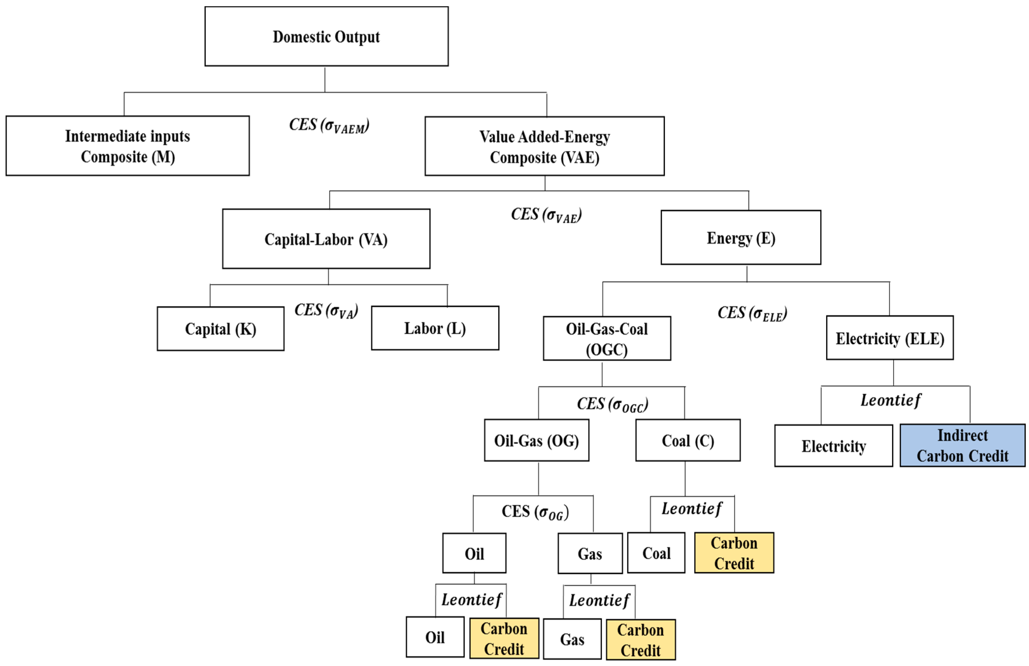
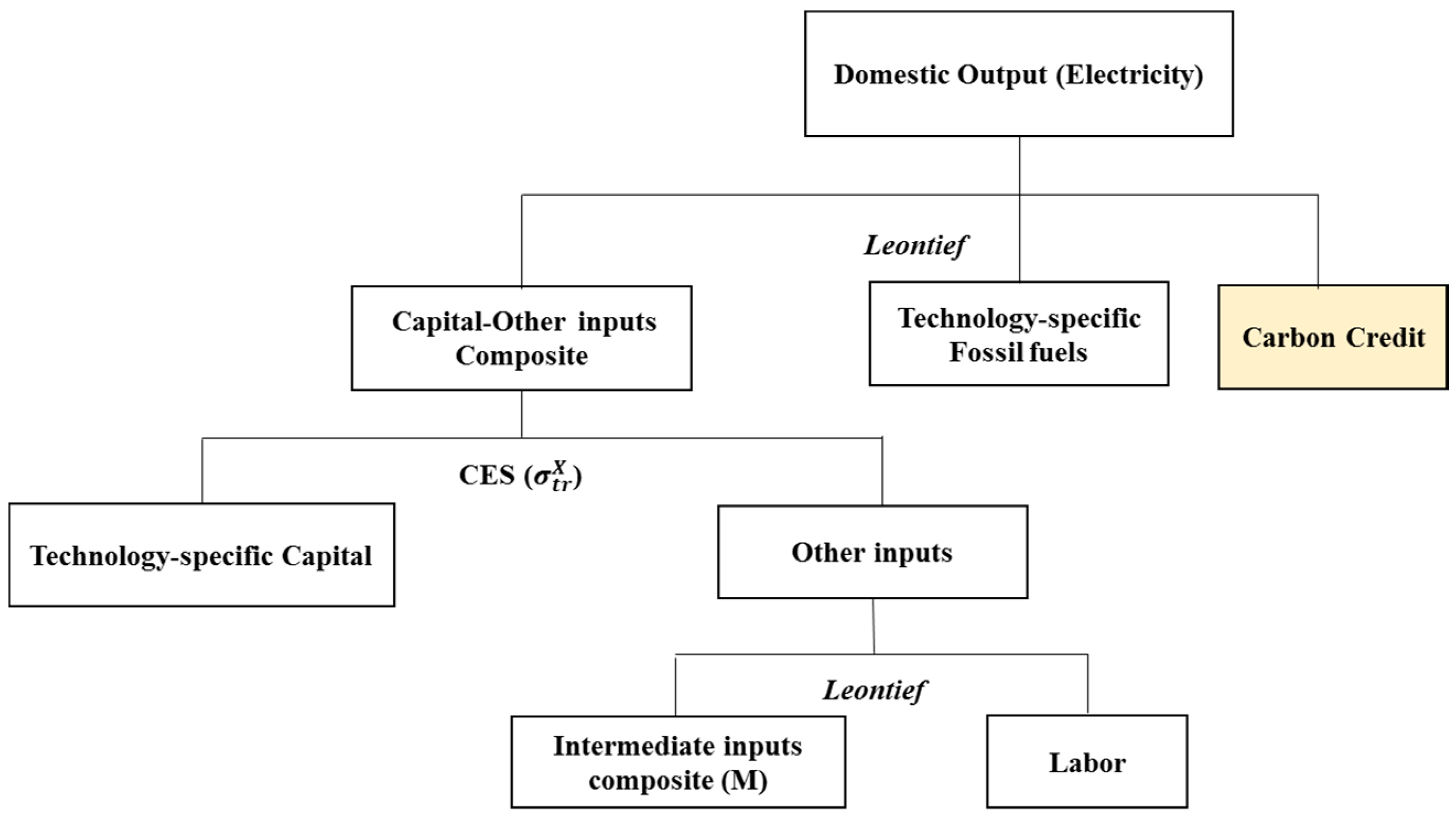
The limitation of this research lies in the assumptions on the key parameters (e.g., the elasticities of substitution in production functions) in building the CGE model. The production of commodities is represented by the nested CES functions. Additionally, the values for substitution elasticities among production factors are adopted from the analysis based on the OECD countries [32]. Further research may require estimation and adaption of the Korean-specific elasticities of substitutions in building the model to draw more reliable simulation results.

References

1. Olivier, J.G.; Janssens-Maenhout, G.; Peters, J.A. Trends in Global CO2 Emissions: 2012 Report; 9279253816; PBL Netherlands Environmental Assessment Agency: Hague, The Netherlands, 2012. [Google Scholar]
2. Bloomberg New Energy Finance. South Korea’s Emissions Trading Scheme; Bloomberg New Energy Finance: NewYork, NY, USA, 2013. [Google Scholar]
3. Sopher, P.; Mansell, A. The World’s Carbon Markets: A Case Study Guide to Emissions Trading: South Korea; Environmental Defense Fund and International Emissions Trading Association: Washington, DC, USA, 2013. [Google Scholar]
4. Park, H.; Hong, W.K. Koreas emission trading scheme and policy design issues to achieve market-efficiency and abatement targets. Energy Policy 2014, 75, 73–83. [Google Scholar] [CrossRef]
5. Hawkins, S.; Jegou, I. Linking Emissions Trading Schemes: Considerations and Recommendations for a Joint EU-Korean Carbon Market; ICTSD Issue Paper; International Ceter for Trade and Sustainable Development (ICTSD): Geneva, Switzerland, 2014. [Google Scholar]
6. Kim, Y.-G.; Lim, J.-S. An emissions trading scheme design for power industries facing price regulation. Energy Policy 2014, 75, 84–90. [Google Scholar] [CrossRef]
7. Lise, W.; Sijm, J.; Hobbs, B.F. The Impact of the EU ETS on Prices, Profits and Emissions in the Power Sector: Simulation Results with the COMPETES EU20 model. Environ. Resour. Econ. 2010, 47, 23–44. [Google Scholar] [CrossRef]
8. Honkatukia, J.; Mälkönen, V.; Perrels, A. Impacts of the European Emission Trade System on Finnish Wholesale Electricity Prices; Discussion Papers in Government Institute for Economic Research; Government Institute for Economic Research Finland: Helsinki, Finland, 2006.
9. Chen, Y.; Sijm, J.; Hobbs, B.F.; Lise, W. Implications of CO2 emissions trading for short-run electricity market outcomes in northwest Europe. J. Regul. Econ. 2008, 34, 251–281. [Google Scholar] [CrossRef]
10. Lund, P. Impacts of EU carbon emission trade directive on energy-intensive industries—Indicative micro-economic analyses. Ecol. Econ. 2007, 63, 799–806. [Google Scholar] [CrossRef]
11. Kemfert, C.; Kohlhaas, M.; Truong, T.; Protsenko, A. The Environmental and Economic Effects of European Emissions Trading. Clim. Policy 2006, 6, 441–455. [Google Scholar] [CrossRef]
12. Hwang, W.-S.; Oh, I.; Lee, J.-D. The Impact of Korea’s Green Growth Policies on the National Economy and Environment. B.E. J. Econ. Anal. Policy 2014, 14, 1585–1614. [Google Scholar] [CrossRef]
13. Hwang, W.-S.; Oh, I.; Lee, J.-D. Assessing the Socio-Economic Effects of Korea’s Nuclear Power Policy. Energy Environ. 2014, 25, 931–952. [Google Scholar] [CrossRef]
14. World Business Council for Sustainable Development; World Resources Institute. The Greenhouse Gas Protocol: A Corporate Accounting and Reporting Standard; World Resources Institute: Geneva, Switzerland, 2001. [Google Scholar]
15. Bebbington, J.; Larrinaga-Gonzalez, C. Carbon Trading: Accounting and Reporting Issues. Eur. Account. Rev. 2008, 17, 697–717. [Google Scholar] [CrossRef]
16. Otte, G.; Prasad, S. GHG emissions accounting. Account. Organ. Soc. 2008, 27, 687–708. [Google Scholar]
17. Government’s Department of Energy and Climate Change (DECC). Climate Change and Energy—Guidance: Sharing Information on Greenhouse Gas Emissions from Local Authority Own Estate and Operations 2013; DECC: London, UK, 2013.
18. Liu, Z.; Dong, H.; Geng, Y.; Lu, C.; Ren, W. Insights into the Regional Greenhouse Gas (GHG) Emission of Industrial Processes: A Case Study of Shenyang, China. Sustainability 2014, 6, 3669–3685. [Google Scholar] [CrossRef]
19. Framework Act on Low Carbon, Green Growth. Available online: http://www.law.go.kr/LSW/lsInfoP.do?lsiSeq=98467&urlMode=engLsInfoR&viewCls=engLsInfoR#0000 (accessed on 10 September 2015). (In Korean)
20. Fabra, N.; Reguant, M. Pass-Through of Emissions Costs in Electricity Markets; National Bureau of Economic Research (NBER): Cambridge, MA, USA, 2013. [Google Scholar]
21. Sijm, J.; Chen, Y.; Hobbs, B.F. The impact of power market structure on CO2 cost pass-through to electricity prices under quantity competition—A theoretical approach. Energy Econ. 2012, 34, 1143–1152. [Google Scholar] [CrossRef]
22. International Emissions Trading Association (IETA). Industry-to-Industry Dialogue on Emissions Trading & Market Readiness: Workbook from the IETA Business Partnership for Market Readiness (B-PMR) Mission in Seoul; IETA: Washington, DC, USA, 2013. [Google Scholar]
23. Internationl Energy Agency (IEA). Energy Statistics of OECD Countries 2014; IEA: Paris, France, 2014. [Google Scholar]
24. Laing, T.; Sato, M.; Grubb, M.; Comberti, C. Assessing the Effectiveness of the EU Emissions Trading System; Centre for Climate Change Economics and Policy (CCCEP): London, UK, 2013. [Google Scholar]
25. Neuhoff, K. Carbon Pricing for Low-Carbon Investment: Executive Summary; DIW Berlin: Berlin, Germany, 2011. [Google Scholar]
26. Xie, X.; Cai, W.; Jiang, Y.; Zeng, W. Carbon Footprints and Embodied Carbon Flows Analysis for China’s Eight Regions: A New Perspective for Mitigation Solutions. Sustainability 2015, 7, 10098–10114. [Google Scholar] [CrossRef]
27. Zhang, D.; Karplus, V.J.; Cassisa, C.; Zhang, X. Emissions Trading in China: Progress and Prospects. Energy Policy 2014, 75, 9–16. [Google Scholar] [CrossRef]
28. International Emissions Trading Association (IETA). China: An Emissions Trading Case Study; IETA: Washington, DC, USA, 2015. [Google Scholar]
29. Zhang, Z.X. Carbon Emissions Trading in China: The Evolution from Pilots to a Nationwide Scheme. Available oneline: http://ssrn.com/abstract=2600909 (accessed on 10 November 2015).
30. Ministry of the Environment (MOE). Scheme Options for Japanese Emissions Trading Scheme Based on Cap and Trade System; MOE: Tokyo, Japan, 2010. [Google Scholar]
31. International Emissions Trading Association (IETA). Tokyo: An Emission Trading Case Study; IETA: Washington, DC, USA, 2015. [Google Scholar]
32. Okagawa, A.; Ban, K. Estimation of Substitution Elasticities for CGE Models. Avaiable online: http://www2.econ.osaka-u.ac.jp/library/global/dp/0816.pdf (accessed on 10 November 2015).
33. Armington, P.S. A Theory of Demand for Products Distinguished by Place of Production. Staff Pap. Int. Monet. Fund 1969, 16, 159–178. [Google Scholar] [CrossRef]
34. Korea Energy Economics Institute (KEEI). 2013 Energy Balance Flow; KEEI: Ulsan, Korea, 2013. [Google Scholar]
35. Greenhouse Gas Inventory & Research Center of Korea (GIR). National Greenhouse Gas Inventory Report of Korea 2013; GIR: Seoul, Korea, 2013. [Google Scholar]
36. Wing, I.S. The Synthesis of Bottom-Up and Top-Down Approaches to Climate Policy Modeling: Electric Power Technologies and the Cost of Limiting U.S. CO2 Emissions. Energy Policy 2006, 34, 3847–3869. [Google Scholar] [CrossRef]
37. Böhringer, C. The Synthesis of Bottom-Up and Top-Down in Energy Policy Modeling. Energy Econ. 1998, 20, 233–248. [Google Scholar] [CrossRef]
38. Böhringer, C.; Löschel, A. Promoting Renewable Energy in Europe: A Hybrid Computable General Equilibrium Approach. Energy J. 2006, 135–150. [Google Scholar] [CrossRef]
39. Kiuila, O.; Rutherford, T.F. The cost of reducing CO2 emissions: Integrating abatement technologies into economic modeling. Ecol. Econ. 2013, 87, 62–71. [Google Scholar] [CrossRef]
40. Böhringer, C.; Rivers, N.J.; Rutherford, T.F.; Wigle, R. Green Jobs and Renewable Electricity Policies: Employment Impacts of Ontario’s Feed-in Tariff. B.E. J. Econ. Anal. Policy 2012, 12, 1–38. [Google Scholar] [CrossRef]
41. Rutherford, T. Lecture Notes on Constant Elasticity Functions; University of Colorado: Denver, CO, USA, 2002; pp. 1–32. [Google Scholar]
42. U.S. Energy Information Administration (EIA). International Energy Outlook 2013; EIA: Washington, DC, USA, 2013. [Google Scholar]
43. U.S. Energy Information Administration (EIA). International Energy Outlook 2014; EIA: Washington, DC, USA, 2014. [Google Scholar]
44. Korea Energy Economics Institute (KEEI). Yearbook of Energy Statistics 2013; KEEI: Ulsan, Korea, 2013. [Google Scholar]
45. Korea Energy Economics Institute (KEEI). Energy Consumption Survey; KEEI: Ulsan, Korea, 2011. [Google Scholar]
46. Labandeira, X.; Labeaga, J.M.; López-Otero, X. Estimation of elasticity price of electricity with incomplete information. Energy Econ. 2012, 34, 627–633. [Google Scholar] [CrossRef]
47. Fan, S.; Hyndman, R.J. The Price Elasticity of Electricity Demand in South Australia. Energy Policy 2011, 39, 3709–3719. [Google Scholar] [CrossRef]
48. Jamil, F.; Ahmad, E. Income and Price Elasticities of Electricity Demand: Aggregate and Sector-wise Analyses. Energy Policy 2011, 39, 5519–5527. [Google Scholar] [CrossRef]
49. Taylor, T.; Schwarz, P.; Cochell, J. 24/7 Hourly Response to Electricity Real-Time Pricing with Up to Eight Summers of Experience. J. Regul. Econ. 2005, 27, 235–262. [Google Scholar] [CrossRef]
50. Jang, E.-K.; Park, M.-S.; Roh, T.-W.; Han, K.-J. Policy instruments for eco-innovation in Asian countries. Sustainability 2015, 7, 12586–12614. [Google Scholar] [CrossRef]
51. Paltsev, S.; Reilly, J.M.; Jacoby, H.D.; Morris, J.F. The Cost of Climate Policy in the United States. Energy Economics 2009, 31, 235–243. [Google Scholar] [CrossRef]
52. Morris, J. Combining a Renewable Portfolio Standard with a Cap-and-Trade Policy: A General Equilibrium Analysis. Master’s Thesis, Massachusetts Institute of Technology, Cambridge, MA, USA, 2009. [Google Scholar]
53. Del Río González, P. The Interaction between Emissions Trading and Renewable Electricity Support Schemes. An Overview of the Literature. Mitig. Adapt. Strateg. Glob. Chang. 2007, 12, 1363–1390. [Google Scholar] [CrossRef]
54. Fischer, C.; Preonas, L. Combining Policies for Renewable Energy: Is the Whole Less than the Sum of Its Parts? Int. Rev. Environ. Resour. Econ. 2010, 4, 51–92. [Google Scholar] [CrossRef]
55. Böhringer, C.; Rosendahl, K.E. Green promotes the dirtiest: On the interaction between black and green quotas in energy markets. J. Regul. Econ. 2010, 37, 316–325. [Google Scholar] [CrossRef]
56. Böhringer, C.; Rosendahl, K.E. Green Serves the Dirtiest: On the Interaction between Black and Green Quotas; Statistics Norway: Oslo, Norway, 2009. [Google Scholar]
57. Mason, S.; Howard, D. Regional Industry Diversity and Its Impact on Regional Unemployment. In Proceedings of the 12th Path to Full Employment/17th National Unemployment Conference, Newcastle, Australia, 2–3 December 2010.
58. Austrailian Bureau of Statistics. A Review of Selected Regional Industrial Diversity Indexes; Austrailian Bureau of Statistics (ABS): Canberra, Austrailia, 2011.
59. Wagner, J.E. Regional Economic Diversity: Action, Concept, or State of Confusion. J. Reg. Anal. Policy 2000, 30, 1–22. [Google Scholar]
60. Van der Werf, E. Production Functions for Climate Policy Modeling: An Empirical Analysis. Energy Econ. 2008, 30, 2964–2979. [Google Scholar] [CrossRef]